Proposal of Wireless Charging Which Enables Magnetic Field Suppression at Foreign Object Location

Abstract

In the wireless power transmission (WPT) to electric vehicles (EVs) in parking lots, there is a risk of abnormal heat generation due to the absorption of the magnetic field in metallic foreign objects. Accordingly, currently available products are equipped with a function that automatically halts power transmission when a metallic foreign object is detected. However, if possible, continuing power transmission while suppressing the magnetic field absorption may be an another solution. Therefore, this paper proposes a novel function which enables wireless power transmission with high efficiency while suppressing the magnetic field absorption of metallic foreign objects. In this study, it was assumed that a metallic foreign body was present in an arbitrary point in a two-dimensional plane and the power transmission was conducted by the phased array WPT. An algorithm using particle swarm optimization (PSO) to search for the optimal combination of the phase and amplitude of the coil input voltages together with coil arrangements, in terms of both magnetic field suppression and transmission efficiency, is proposed. The simulation was performed with the lower efficiency boundary set as 85% and the load power set as 11 kW, in reference to the SAE J2954 standard. As a result, it was confirmed that the magnetic field suppression effect increased in accordance with the increase in the number of transmission (Tx) coils, thus indicating the effectiveness of the proposed algorithm.

1. Introduction

In recent years, the use of electric vehicles (EVs) has increased and is expected to be more widespread in the future due to changes in the social climate. The charging units currently installed in EVs charge the vehicle battery by the connection between the charger and the charging port of the vehicle. However, batteries installed in EVs have a relatively low capacity and require frequent recharging. Hence, the burden of manual power transmission and the risk of electric shock [1] should be minimized.

Wireless power transfer (WPT) has attracted considerable attention as a potential solution to the above-mentioned problem. As a WPT method for EVs, the magnetic resonance coupling (MRC) method [2] has attracted significant research attention due to its long transmission distance and low risk of harmful exposure to humans [3,4,5,6].

However, with wireless power transfer via magnetic resonance coupling (MRC-WPT), energy is transmitted by the coupling of magnetic fields between coils, which causes the excessive heating of interfering objects such as conductors and magnetic materials in the vicinity of the coils. This leads to a reduction in the efficiency of the WPT. The losses due to these interferents are eddy current losses for conductors and hysteresis losses for magnetic materials.

Therefore, the SAE J2954 standard, which is an international standard for the WPT of EVs, specifies that metal object detection (MOD) should be performed to ensure safe operation considering foreign objects and WPT should be stopped if necessary [7]. This is shown in Figure 1a,b.

MOD methods could be categorized in three types [8,9], system parameter-based detection, wave detection and field-based detection methods; the use of search coil arrays [10,11], thermal cameras [12] and tunneling magnetoresistive (TMR) sensors [13] as the main sensors has been proposed. Currently available products are also equipped with functionality designed to halt WPT when a metallic foreign body is detected, e.g., WiTricity [14], DAIHEN D-Broad EV [15] and Qualcomm Halo [16].

On the other hand, as per the SAE J2954 standard, the prevention of dangerous increases in the temperature of the foreign object by appropriately controlling the magnetic field in the transmission (Tx) coil is allowed as an alternative approach. In particular, this approach can be characterized by continuous WPT with the maximum suppression of the magnetic field absorption of the foreign object. This is shown in Figure 1c,d. However, such an approach has not been extensively investigated, as discussed below.

First, we clarify the problem settings. We considered WPT from the Tx coil to the EV on a flat road surface, such as a parking lot. To control the magnetic field distribution in MRC-WPT, the use of a phased array coil, as the Tx coil, is effective. Therefore, this is the problem of (1) suppressing the magnetic field at the position of the metallic foreign object and (2) maintaining high transmission efficiency of wireless power transmission, supposing that the metallic foreign object exists in an arbitrary point on the road surface between the Tx coil array and the Rx coil. As follows, there is no existing study on magnetic field control using phased array WPT that deals with such problem settings.

Existing studies on magnetic field control using phased array WPT can be categorized into two types. First, there are studies on suppressing the magnetic field in the surrounding space while transferring power by focusing the magnetic field to the Rx coil [17,18,19,20]. Unlike the case where the magnetic field is suppressed only at an arbitrary point on a two-dimensional plane, the magnetic field is suppressed in the entire space, in the cases. Second, there are studies on selective power transfer to multiple Rx coils by controlling the magnetic field [21,22,23,24]. In these studies, the position of the untargeted Rx coil where the magnetic field should be suppressed is given, so the problem setting is different from the case where the position of the point where the magnetic field should be suppressed is unknown in the two-dimensional plane. A comparison with existing studies on magnetic field control using phased array WPT is summarized in

Table 1. Comparison among existing studies on magnetic Field control using phased array WPT.

	Focusing the Magnetic Field				Selective Power Transfer				This Study
References	[17]	[18]	[19]	[20]	[21]	[22]	[23]	[24]	–
Number of Tx coils	2	3	2	5	2	4	10	10	2–5
Dimensions of the Tx coil array	3D	3D	1D	2D	1D	1D	1D	1D	2D
Magnetic field suppression in the surrounding space	yes	yes	yes	yes	no	no	no	no	no
Magnetic field suppression at single point	no	no	no	no	yes	yes	yes	yes	yes
The point where magnetic field should be suppressed	–	–	–	–	definite	definite	definite	definite	indefinite
Magnetic field suppression at any point in the 2D plane	–	–	–	–	no	no	no	no	yes

.

Therefore, it could be said that the problem settings of phased array WPT that enable efficient WPT while suppressing the magnetic field at an arbitrary point in the two-dimensional plane assuming a road surface, where the metallic foreign object may exist, are a novelty.

In summary, this study makes two academic contributions. First, the problem of highly efficient WPT with magnetic field suppression at an arbitrary point in a two-dimensional plane using phased array WPT is addressed. Second, to solve this new problem, particle swarm optimization (PSO) was applied with an evaluation function that considered both the power transmission efficiency and magnetic field suppression. The proposed algorithm searches for the optimal combination of the phase and amplitude of the input voltage of each Tx coil with respect to each coil arrangement and magnetic field suppression position. It should be noted that the arrangement of the Tx coil array has rarely been addressed in previous studies.

To make the problem simple, the detection of metallic foreign objects and Rx coil was presumed to be implemented and is not addressed in this paper. The detection of metallic foreign objects could be realized by previously mentioned methods [10,11,12,13]. On the other hand, the detection of the Rx coil could be realized by, for instance, using the most promising method whereby the Tx coils are also used as sensors [25,26], on which the authors have been also working [27,28]. This method has also been applied to EVs [29].

In addition, we plan to reference a database of various input voltage combinations according to the positions of the Rx coil and the metallic foreign object, in order to respond in real time by simply switching the input voltage.

2. Methodology

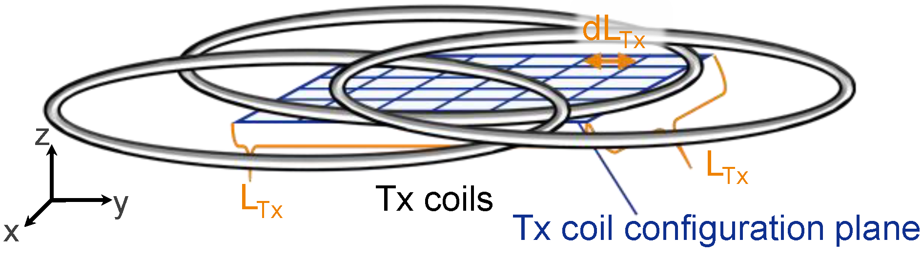
2.1. Directivity Control of Magnetic Field by Phased Array Coils

In the case of a phased array Tx coil, the magnetic field distribution can be regarded as a superposition of the magnetic field distribution generated by a single coil and the magnetic field distribution can be controlled by controlling the current flowing through the coil. Therefore, the magnetic field can be suppressed at the target position by appropriately setting the number and arrangement of Tx coils and controlling the phase and amplitude of the current flowing through each Tx coil.

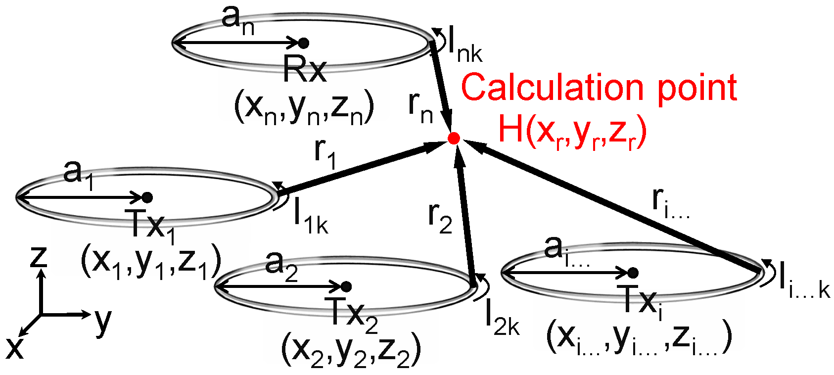
2.2. Calculation of Transmission Efficiency and Magnetic Field Strength

2.2.1. Transmission Efficiency

In MRC-WPT, the efficiency of WPT is most commonly derived from electric circuit theory using an equivalent circuit. However, it is difficult to incorporate the effects of mutual interference between the interferents and coils into the circuit model when deriving the efficiency. Therefore, we assumed that the magnetic field in the area of the interfering object was reduced by the magnetic field control, to eliminate the effect of mutual interference. Then, we derived the efficiency approximately from the general circuit equation. The equivalent circuit of the phased array WPT is shown in Figure 2. Here, $n-1$ Tx coils, one Rx coil and n total number of coils are displayed. $R_i$ is the coil resistance, $Z_L$ is the load resistance, $C_i$ is the capacitance of the capacitor, $L_i$ is the self-inductance of the coil and $L_{ij}$ is the mutual inductance between the coils. The input voltage of each coil is $V_i$ and the current is $I_i$. It should be noted that $i,j=1,2,\dots ,n$.

The circuit equation of the phased array WPT shown in Figure 2 can be expressed as Equation (1).

$$\left[\begin{array}{c}{V}_1\\ ⋮\\ V_{n-1}\\ 0\end{array}\right]=\left[\begin{array}{ccc}{R}_1+j(\omega L_1-\frac{1}{\omega C_1})& \cdots & j\omega L_{1n}\\ ⋮& \ddots & ⋮\\ j\omega L_{n-11}& \cdots & j\omega L_{n-1n}\\ j\omega L_{n1}& \cdots & R_n+Z_L+j(\omega L_n-\frac{1}{\omega C_n})\end{array}\right]\left[\begin{array}{c}{I}_1\\ ⋮\\ I_{n-1}\\ I_n\end{array}\right]$$

(1)

Given that MRC-WPT assumes a resonance state of each coil, the reactance arising from $L_i$ and $C_i$ is nullified and the circuit equation is Equation (2).

$$\left[\begin{array}{c}{V}_1\\ ⋮\\ V_{n-1}\\ 0\end{array}\right]=\left[\begin{array}{ccc}{R}_1& \dots & j\omega L_{1n}\\ ⋮& \ddots & ⋮\\ j\omega L_{n-11}& \dots & j\omega L_{n-1n}\\ j\omega L_{n1}& \dots & R_n+Z_L\end{array}\right]\left[\begin{array}{c}{I}_1\\ ⋮\\ I_{n-1}\\ I_n\end{array}\right]$$

(2)

To simplify the equation, the input voltage of each coil is represented by $\mathit{V}$, the impedance matrix as $\mathit{Z}$ and the current of each coil as $\mathit{I}$. Thus, Equation (2) can be expressed as Equation (3).

$$\begin{array}{cc}\hfill \mathit{V}& =\mathit{ZI}\hfill \end{array}$$

(3)

In this study, it was assumed that the phase and amplitude of the input voltage of each Tx coil could be independently controlled. The current $\mathit{I}$ can be obtained from Equation (4) by multiplying both sides by the inverse matrix ${\mathit{Z}}^{-\mathbf{1}}$ of the impedance matrix $\mathit{Z}$.

$$\begin{array}{cc}\hfill \mathit{I}& ={\mathit{Z}}^{-\mathbf{1}}\mathit{V}\hfill \end{array}$$

(4)

Thereafter, the power of each coil is derived from Equation (5) using the calculated current values and the power transmission efficiency from all Tx coils to Rx coil is calculated with Equation (6). Moreover, $P_{Tx}$ is the sum of the input power of each Tx coil and $P_{Rx}$ is the load power of the Rx coil. Neumann’s formula is used to calculate the mutual inductance.

$$\begin{array}{cc}\hfill P_{Rx}=\frac{1}{2}{Z}_L{\left|I_n\right|}^2& ,P_{Tx}=\frac{1}{2}\sum _{k=1}^{n-1}Re[V_k·\overline{I_k}]\hfill \end{array}$$

(5)

$$\begin{array}{cc}\hfill \eta & =\frac{P_{Rx}}{P_{Tx}}\hfill \end{array}$$

(6)

2.2.2. Magnetic Field Strength

The magnetic field generated by the coil can be obtained with the Biot–Savart law. The calculation of the Biot–Savart law is approximated by numerical integration as follows: the current $I_{ik}$ flowing through coil i is represented by Equation (7), where $A_i$ is the amplitude of the current and ${\theta }_i$ is the phase difference of the current. $T_{div}$ is the number of divisions in one cycle of the time-varying magnetic field, where $k=1,2,\dots ,T_{div}$.

$$\begin{array}{cc}\hfill I_{ik}& =A_{i}cos\left(\frac{2\pi }{T_{div}}k+{\theta }_i\right)+j{A}_{i}sin\left(\frac{2\pi }{T_{div}}k+{\theta }_i\right)\hfill \end{array}$$

(7)

As shown in Figure 3, if the coordinates of the magnetic field calculation point are ($x_r,y_r,z_r$) and the coordinates of the center of the coil i are ($x_i,y_i,z_i$), the distance $r_i$ from the coordinates of the current element of coil i to the magnetic field calculation point can be calculated using Equation (9).

$$\begin{array}{cc}\hfill X& =x_r-x_i,Y=y_r-y_i,Z=z_r-z_i\hfill \end{array}$$

(8)

$$\begin{array}{cc}\hfill r_i& =[X^2+Y^2+Z^2+{a_i}^2-2a_i\left\{Xcos\left(\frac{2\pi }{m}l\right)+Ysin\left(\frac{2\pi }{m}l\right)\right\}{]}^{\frac{1}{2}}\hfill \end{array}$$

(9)

where $a_i$ is the radius of the coil i, in the case of $n-1$ Tx coils, one Rx coil and a total of n coils; $i=1,2,\dots ,n$. In addition, m is the number of divisions of the magnetic field integral and $l=1,2,\dots ,m$.

Given that multiple coils were here used, the magnetic fields generated by each coil were composited. Therefore, the magnetic fields generated by each coil were calculated using Equations (10)–(12) and the composite vector in each of the x-, y- and z-directions was obtained. Moreover, N is the number of turns generated by the coil.

$$\begin{array}{cc}\hfill H_{xk}& =\sum _{i=1}^{n}N\frac{I_{ik}}{4\pi }\left[\sum _{l=1}^m\frac{Z{a}_{i}cos\left(\frac{2\pi }{m}l\right)·\frac{2\pi }{m}}{r_i^3}\right]\hfill \end{array}$$

(10)

$$\begin{array}{cc}\hfill H_{yk}& =\sum _{i=1}^{n}N\frac{I_{ik}}{4\pi }\left[\sum _{l=1}^m\frac{Z{a}_{i}sin\left(\frac{2\pi }{m}l\right)·\frac{2\pi }{m}}{r_i^3}\right]\hfill \end{array}$$

(11)

$$\begin{array}{cc}\hfill H_{zk}& =\sum _{i=1}^{n}N\frac{I_{ik}}{4\pi }\left[\sum _{l=1}^m\frac{a_i\left\{a_i-Xcos\left(\frac{2\pi }{m}l\right)-Ysin\left(\frac{2\pi }{m}l\right)\right\}·\frac{2\pi }{m}}{r_i^3}\right]\hfill \end{array}$$

(12)

The norm of the 3D vector, which is the composite vector of the x-, y- and z-direction magnetic fields at time k, is then calculated using Equation (13).

$$\begin{array}{cc}\hfill H_{Normk}& =\sqrt{{Re\left(H_{xk}\right)}^2+{Re\left(H_{yk}\right)}^2+{Re\left(H_{zk}\right)}^2}\hfill \end{array}$$

(13)

Since the magnetic field generated by the MRC-WPT is time-varying due to the fact that the input voltage is an alternating current (AC), we calculated the root mean square of the time series data in each direction of the magnetic field composite vector and obtained the effective value represented as magnetic field strength $H_{RMS}$.

$$\begin{array}{cc}\hfill H_{RMS}& =\sqrt{\frac{{\sum }_{k=1}^{T_{div}}{H_{Normk}}^2}{T_{div}}}\hfill \end{array}$$

(14)

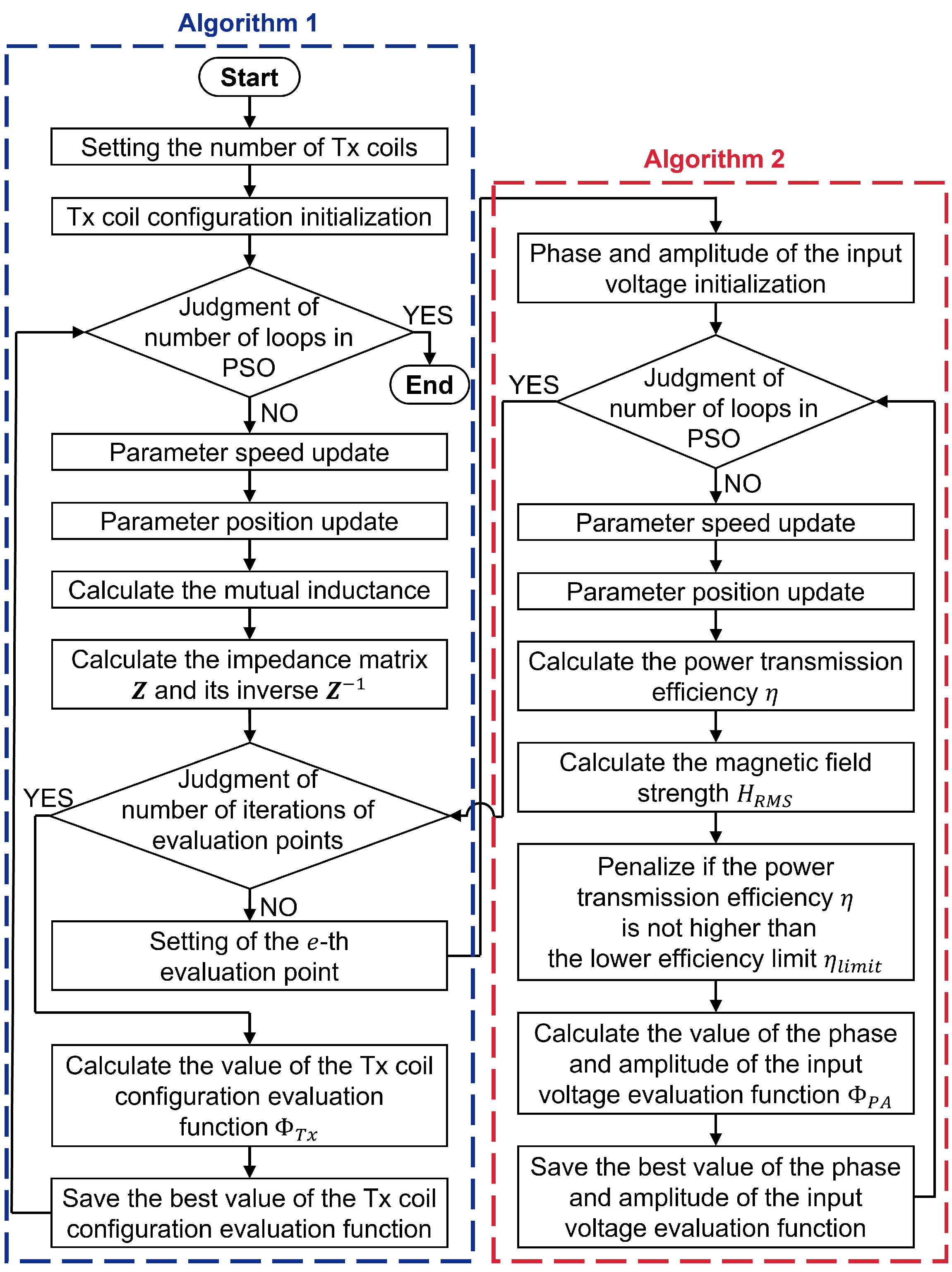
2.3. Parameter Optimization of Phased Array WPT Function

In this study, we assumed a case wherein a single metallic foreign body was detected in a specified area on a two-dimensional plane during WPT to an EV in a parking lot. The metallic foreign object was presumed to be located directly above the ground at a certain height from the buried Tx coil which is a specified area on a two-dimensional plane. Moreover, it was assumed that a single metallic foreign body could be detected using existing methods, thus allowing the coordinate information of that single point to be obtained. Therefore, the proposed function made possible highly efficient WPT while realizing magnetic field suppression at any single point in the two-dimensional plane.

To realize the proposed functionality, it is necessary to determine the input voltage according to the coordinates of the metallic foreign body within the arrangement of the Tx coils that constitutes the phased array coil, given the specifications of the Tx and Rx coils. The input voltage to each coil are controllable parameters that can be freely selected according to the coordinate information of the metallic foreign body, while the coil configuration is a fixed and uncontrollable parameter that is determined at the design stage. Considering these facts, the methods to determine these parameters are described as follows.

The Tx coil is arranged in the position where the center coordinates of each Tx coil correspond to one of the grid points of grid spacing $d{L}_{Tx}$ in a planar area with a side length $L_{Tx}$ centered at (0, 0, 0) mm, as shown in Figure 4.

The Tx coil configuration is evaluated in terms of the power transmission efficiency and magnetic field suppression (in the planar area where suppression is performed). The evaluation of the transmission efficiency and the magnetic field suppression is performed for the grid points in the planar area with a grid spacing of $d{L}_{Ev}$ and a side length of $L_{Ev}$ centered at (0, 0, $h_{Ev}$) mm, as shown in Figure 5.

In this paper, this plane is referred to as the evaluation plane and the grid points are referred to as evaluation points.

In particular, for a given Tx coil configuration, a combination of the phase and amplitude of the input voltage to each coil that achieves both high transmission efficiency and magnetic field suppression is obtained for each evaluation point on the evaluation plane and the sum of the transmission efficiency and magnetic field strength obtained for all evaluation points is used as the evaluation value for the given Tx coil configuration. By iteratively performing these optimization processes, the optimal Tx coil configuration and appropriate combination of the phase and amplitude of the input voltage to each coil for every evaluation point can be derived.

However, it is difficult to perform such an optimization analytically. Therefore, the use of PSO [30], which is a common technique for determining the quasi-optimal solution in multi-objective optimization within a short time-period, could be effective. The PSO algorithm uses multiple particles to perform the search. Based on the information of the shared particles, the update values are obtained from Equations (15) and (16) and the search is repeated to obtain the quasi-optimal solution of the evaluation function. The inertia constant $W^{k+1}$ decreases linearly at the end of the search according to Equation (17) and local search is performed. Moreover, $W_{max}$ is the inertia constant at the start of the search; $W_{min}$ is the inertia constant at the end of the search; $i(=1,2,\dots ,Pn)$ is the particle number; $j(=1,2,\dots ,n)$ is the coil number; k is the number of search updates; and $k_{max}$ is the number of searches.

$$\begin{array}{cc}\hfill {v_{ij}}^{k+1}& =W^{k+1}·{v_{ij}}^k-C_1·ran{d}_{1ij}·({pbes{t}_{ij}}^k-{x_{ij}}^k)\hfill \\ \hfill & -C_2·ran{d}_{2ij}·({gbes{t}_j}^k-{x_{ij}}^k)\hfill \end{array}$$

(15)

$$\begin{array}{cc}\hfill {x_{ij}}^{k+1}& ={x_{ij}}^k+{v_{ij}}^{k+1}\hfill \end{array}$$

(16)

$$\begin{array}{cc}\hfill W^{k+1}& =\frac{k_{max}-(k+1)}{k_{max}}·(W_{max}-W_{min})+W_{min}\hfill \end{array}$$

(17)

The parameter optimization algorithm using PSO is shown in Figure 6 and the details are described as follows. The detailed procedure of the Tx coil configuration optimization algorithm is shown in the pseudo code of Algorithm 1. The detailed procedure of the input voltage optimization algorithm to each Tx coil is shown in the pseudo code of Algorithm 2.

A Tx coil configuration is assigned to each particle (i.e., coil configuration particle). Then, the coil configuration particle is evaluated in terms of both transmission efficiency and magnetic field suppression over the evaluation plane. This could be realized by following process.

First, a combination of the input voltage to each coil is also assigned to each particle (i.e., input voltage combination particle). Specifically, the input voltage assigned to each particle corresponds to $\mathit{V}$, the input voltage of each Tx coil in Equation (3) and the power transmission efficiency $\eta$ is calculated using Equations (3)–(6). The magnetic field strength $H_{RMS}$ at a single evaluation point on the evaluation plane is calculated from the current $\mathit{I}$ of each coil using Equations (7)–(14). Then, at each evaluation point on the evaluation plane, each input voltage combination particle is evaluated as the weighted sum of the inverse of the corresponding transmission efficiency $\eta$ and the magnetic field strength $H_{RMS}$ from the evaluation function (18). Here, $\alpha$ is the weight factor determining the balance between the magnetic field strength and transmission efficiency and $\beta$ is the weight used to normalize the efficiency and field strength weights. The power transmission efficiency $\eta$ is required to be greater than or equal to the lower efficiency limit ${\eta }_{limit}$; otherwise, a penalty is imposed and no particle is selected.

$$\begin{array}{cc}\hfill {\Phi }_{PA}& =(1-\alpha )·\beta ·\frac{1}{\eta }+\alpha ·H_{RMS}\hfill \end{array}$$

(18)

Considering the evaluation results, the input voltage to each coil of the particle with the best value in the group after a specified number of searches $k_{max}$ is selected for power transmission. This optimization is repeated for all evaluation points on the evaluation plane.

Finally, each coil configuration particle is evaluated as the sum of all evaluation values of the selected input voltage combination particles at all evaluation points. This is expressed as (19). Here, $En$ is the total number of evaluation points $e=1,2,\dots ,En$; and ${\eta }_e$ and $H_{RMS,e}$ refer to the power transmission efficiency $\eta$ and magnetic field strength $H_{RMS}$ at the e-th evaluation point, respectively.

$$\begin{array}{cc}\hfill {\Phi }_{Tx}& =(1-\alpha )·\beta ·\sum _{e=1}^{En}\frac{1}{{\eta }_e}+\alpha ·\sum _{e=1}^{En}{H}_{RMS,e}\hfill \end{array}$$

(19)

The Tx coil configuration of the particle with the best value in the group after a specified number of searches $k_{max}$ is selected as the Tx coil configuration of the WPT function.

The pseudo code for Tx coil configuration optimization using PSO is shown in Algorithm 1. The pseudo code for input voltage optimization using PSO is shown in Algorithm 2.

Algorithm 1. Pseudo code of Tx coil configuration optimization using PSO.

Input:  Simulation parameters Output:  Best Tx coil configuration, the optimal input voltage ${\mathit{V}}_e$ to each Tx coil at the e-th evaluation point, the power transmission efficiency ${\eta }_e$ at the e-th evaluation point and the magnetic field strength $H_{RMS,e}$ at the e-th evaluation point; $e(=1\dots En)$ is the evaluation point number 1: The center coordinates of each Tx coil are assigned to each particle; $i(=1\dots P_n)$ is the particle number; $j(=1\dots n)$ is the coil number; $k(=1\dots k_{max})$ is the number of search updates 2: Initialize particle swarm ${v_{ij}}^0,{x_{ij}}^0,{pbes{t}_i}^0$ and ${gbest}^0$ 3: for$k=1\dots k_{max}$do 4:     Calculate inertia according to (17) 5:     for $i=1\dots P_n$ do 6:         for $j=1\dots n$ do 7:             Calculate particle velocity in x-coordinate according to (15) 8:             Calculate particle velocity in y-coordinate according to (15) 9:             Calculate particle position in x-coordinate according to (16) 10:           Calculate particle position in y-coordinate according to (16) 11:        end for 12:        Calculate the mutual inductance according to Neumann’s formula 13:        Calculate the impedance matrix $\mathbf{Z}$ according to (2) and its inverse ${\mathbf{Z}}^{-\mathbf{1}}$ 14:        for $e=1\dots En$ do 15:           Optimization of the phase and amplitude of input voltage to the coil configuration at each evaluation point according to Algorithm 2 16:           Algorithm 2 returns the optimal input voltage $\mathbf{V}$ to each Tx coil, the power transmission efficiency $\eta$ and the magnetic field strength $H_{RMS}$ at the e-th evaluation point. 17:           The optimal input voltage $\mathbf{V}$ to each Tx coil, the power transmission efficiency $\eta$ and the magnetic field strength $H_{RMS}$ at the e-th evaluation point are named ${\mathit{V}}_e$, ${\eta }_e$ and $H_{RMS,e}$, respectively 18:        end for 19:        Calculate the value of the Tx coil configuration evaluation function ${\Phi }_{Tx}$ according to (19) 20:        if ${\Phi }_{Tx}\left({x_i}^{k+1}\right)<{\Phi }_{Tx}\left({pbes{t}_i}^k\right)$ then 21:           ${pbes{t}_i}^{k+1}={x_i}^{k+1}$ 22:        else 23:           ${pbes{t}_i}^{k+1}={pbes{t}_i}^k$ 24:        end if 25:    end for 26:    $gbes{t}^{k+1}={pbes{t}_{i_g}}^{k+1}$ 27:    where ${\displaystyle i_g=arg\underset{i}{min}{\Phi }_{Tx}\left({pbes{t}_{i_g}}^{k+1}\right)}$ 28: end for

Algorithm 2. Pseudo code of the input voltage optimization using PSO.

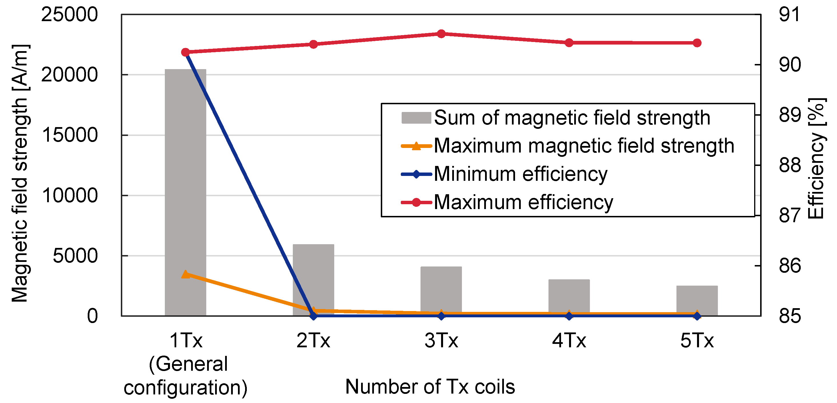
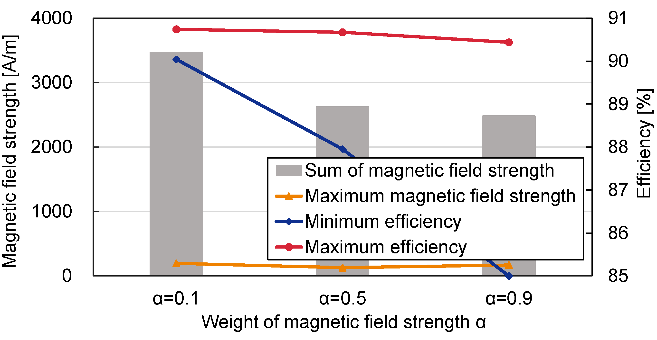
Input:  Coordinates of all coils, coordinates of an evaluation point and inverse of impedance matrix ${\mathit{Z}}^{-\mathbf{1}}$; these are given by Algorithm 1 Output:  Best combination of the phase and amplitude of input voltage $\mathit{V}$ to each Tx coil, the power transmission efficiency $\eta$ and the magnetic field strength $H_{RMS}$ 1: The phase and the amplitude of input voltage to each coil are assigned to each particle; $i(=1\dots P_n)$ is the particle number; $j(=1\dots n)$ is the coil number; $k(=1\dots k_{max})$ is the number of search updates 2: Initialize particle swarm ${v_{ij}}^0,{x_{ij}}^0,{pbes{t}_i}^0$ and ${gbest}^0$ 3: for$k=1\dots k_{max}$do 4:    Calculate inertia according to (17) 5:    for $i=1\dots P_n$ do 6:      for $j=1\dots n$ do 7:         Calculate particle velocity of the phase of the input voltage according to (15) 8:         Calculate particle velocity of the amplitude of the input voltage according to (15) 9:         Calculate particle position of the phase of the input voltage according to (16) 10:         Calculate particle position of the amplitude of the input voltage according to (16) 11:      end for 12:      Calculate the input voltage $\mathit{V}$ according to (3) 13:      Calculate the input current $\mathit{I}$ according to (4) 14:      Calculate the load power of the Rx coil $P_{Rx}$ according to (5) 15:      Adjust the amplitude of the input voltage so that the load power $P_{Rx}$ becomes equal to the set value $P_L$ 16:      Calculate the input power $P_{Tx}$, the load power $P_{Rx}(=P_L)$ and the power transmission efficiency $\eta$ according to (5), (6) 17:      Calculate the magnetic field strength $H_{RMS}$ according to (7)–(14) 18:      Calculate the value of the phase and amplitude of the input voltage evaluation function ${\Phi }_{PA}$ according to (18) 19:      if $\eta <{\eta }_{limit}$ then 20:         ${\Phi }_{PA}\left({x_i}^{k+1}\right)+=penalty$ 21:      end if 22:      if ${\Phi }_{PA}\left({x_i}^{k+1}\right)<{\Phi }_{PA}\left({pbes{t}_i}^k\right)$ then 23:          ${pbes{t}_i}^{k+1}={x_i}^{k+1}$ 24:      else 25:          ${pbes{t}_i}^{k+1}={pbes{t}_i}^k$ 26:      end if 27:    end for 28:    $gbes{t}^{k+1}={pbes{t}_{i_g}}^{k+1}$ 29:    where ${\displaystyle i_g=arg\underset{i}{min}{\Phi }_{PA}\left({pbes{t}_{i_g}}^{k+1}\right)}$ 30: end for 31: return$gbest$ (best combination of the phase and amplitude of input voltage $\mathit{V}$ to each Tx coil), the power transmission efficiency $\eta$ and the magnetic field strength $H_{RMS}$

3. Simulation

3.1. Simulation Conditions

First, the height $h_{Ev}$ from the plane of the Tx coil to the evaluation plane was set as 10 mm. Thereafter, the grid spacing $d{L}_{Ev}$ of the evaluation plane was set as 100 mm, the length of one side $L_{Ev}$ was set as 600 mm and the total number of evaluation points $En$ was set as 49 for input voltage optimization. Here, the total number of evaluation points was 49 because each side had 7 evaluation points due to the fact that the length of one side of the evaluation plane $L_{Ev}$ was 600 mm. In addition, the grid spacing $d{L}_{Tx}$ of the Tx coil configuration plane was 10 mm and the length of one side $L_{Tx}$ was 200 mm.

From two to five Tx coils and one Rx coil were installed, the load power $P_L$ was 11 kW and the lower efficiency limit ${\eta }_{limit}$ was set as 85%. The load power and the lower efficiency limit were based on the values specified in the SAE J2954 standard [7]. Note that SAE J2954 actually sets the efficiency of the entire system at 85%. Therefore, efficiency loss in the power electronics converter also had to be considered. However, since this study is still in the proof-of-principle stage, the efficiency losses appearing other than from coil to coil were neglected as approximation. We think this would not cause many problems because the latest version of the commercial converter had a sufficient efficiency of about 96% [31,32]. The conditions including these neglected losses will be considered in the future when the actual system will be developed. The height $h_{Rx}$ from the plane of the Tx coil to the Rx coil was 150 mm and the Rx coil was fixed at (0, 0, 150) mm. The coils used in this study had the same shape with radius a of 150 mm and 70 turns N. The coil material was copper wire and litz wire was not used. Moreover, the resonance frequency f was 85 kHz, $R=R_1=\dots R_n$, $L=L_1=\dots L_n$ and $C=C_1=\dots C_n$ were satisfied. The parameters of the coils were simulated by IE3D, a three-dimensional electromagnetic field analysis simulator. The overlap of the Tx coils was allowed assuming the solution such as slightly bending either coil where the coils were overlapping [33].

The weights $\alpha$ determining the weighting balance between the magnetic field strength and transmission efficiency in the evaluation function for Tx coil arrangement and input voltage optimization were set as $\alpha =0.1,0.5$ and 0.9, which correspond to the efficiency prioritization, same prioritization and magnetic field suppression prioritization, respectively. The weight $\beta$ for normalizing the weights of the efficiency and field strength was set as $\beta =1000$.

The simulation parameters are listed in

Table 2. Simulation parameters.

Parameter	Value	Dimension
Grid spacing of the Tx coil configuration plane $d{L}_{Tx}$	10	mm
Side length of the Tx coil configuration plane $L_{Tx}$	200	mm
Grid spacing of the evaluation plane $d{L}_{Ev}$	100	mm
Side length of the evaluation plane $L_{Ev}$	600	mm
Evaluation plane height $h_{Ev}$	10	mm
Tx–Rx Gap $h_{Rx}$	150	mm
Frequency f	85	kHz
Coil material (copper wire)	1.3 × ${10}^{-6}$	H/m
Coil radius a	150	mm
Coil turn N	70	turn
Coil resistance R	5	$\Omega$
Coil inductance L	2.0	mH
Coil capacitance C	1.7	nF
Coil Q-value	213
Load resistance $Z_L$	50	$\Omega$
Load power $P_L$	11	kW
Lower transmission efficiency limit ${\eta }_{limit}$	85	%
Number of Tx coils	2–5	number
Weight between magnetic field strength and power transmission efficiency $\alpha$	0.1, 0.5, 0.9
Weight for normalization $\beta$	1000

.

Table 3. Parameters of PSO.

Parameter	Value
	Coil Configuration	Phase and Amplitude
Number of particles $Pn$	200	200
Number of loops $k_{max}$	300	200
Maximum inertia	0.6	0.6
Factor $W_{max}$
Minimum inertia	0.3	0.3
Factor $W_{min}$
Weighting factor $C_1$	2.0	1.0
Weighting factor $C_2$	1.5	1.7

lists the parameters of PSO used in the optimization.

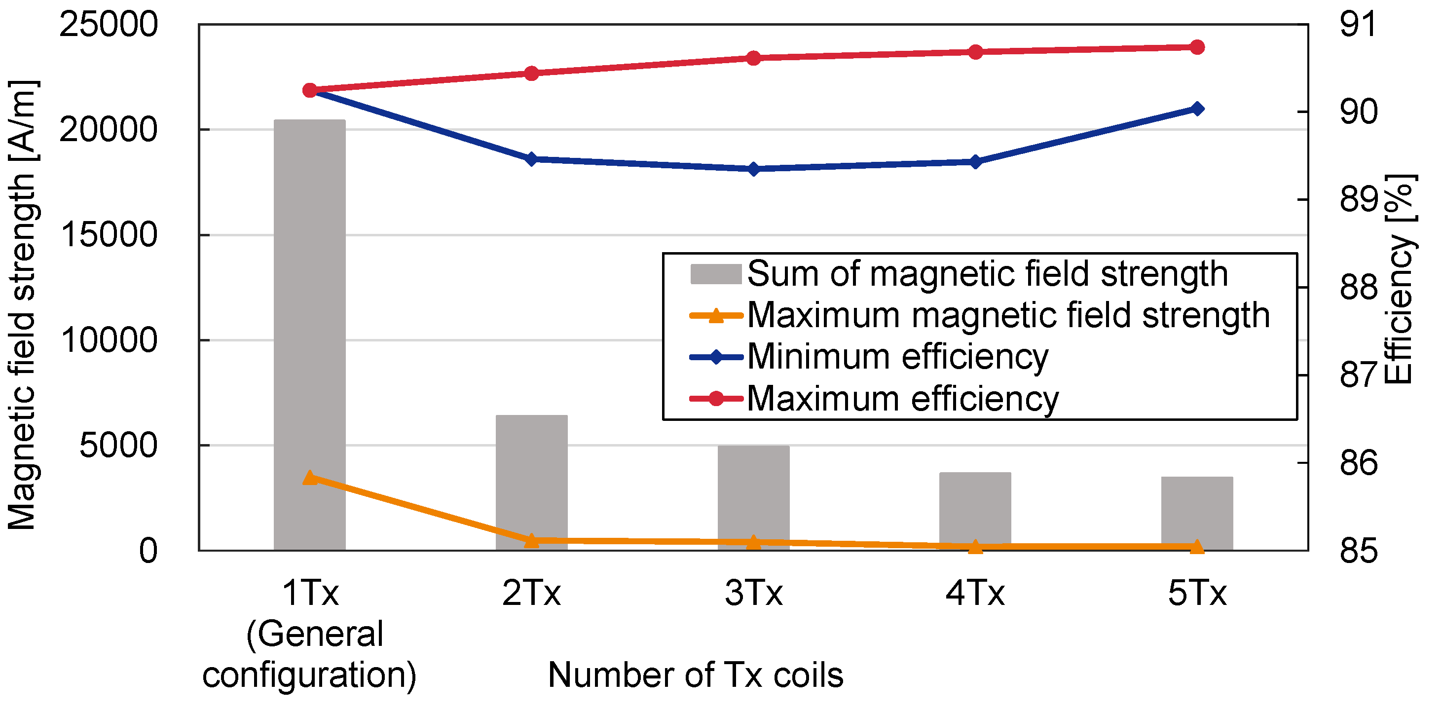
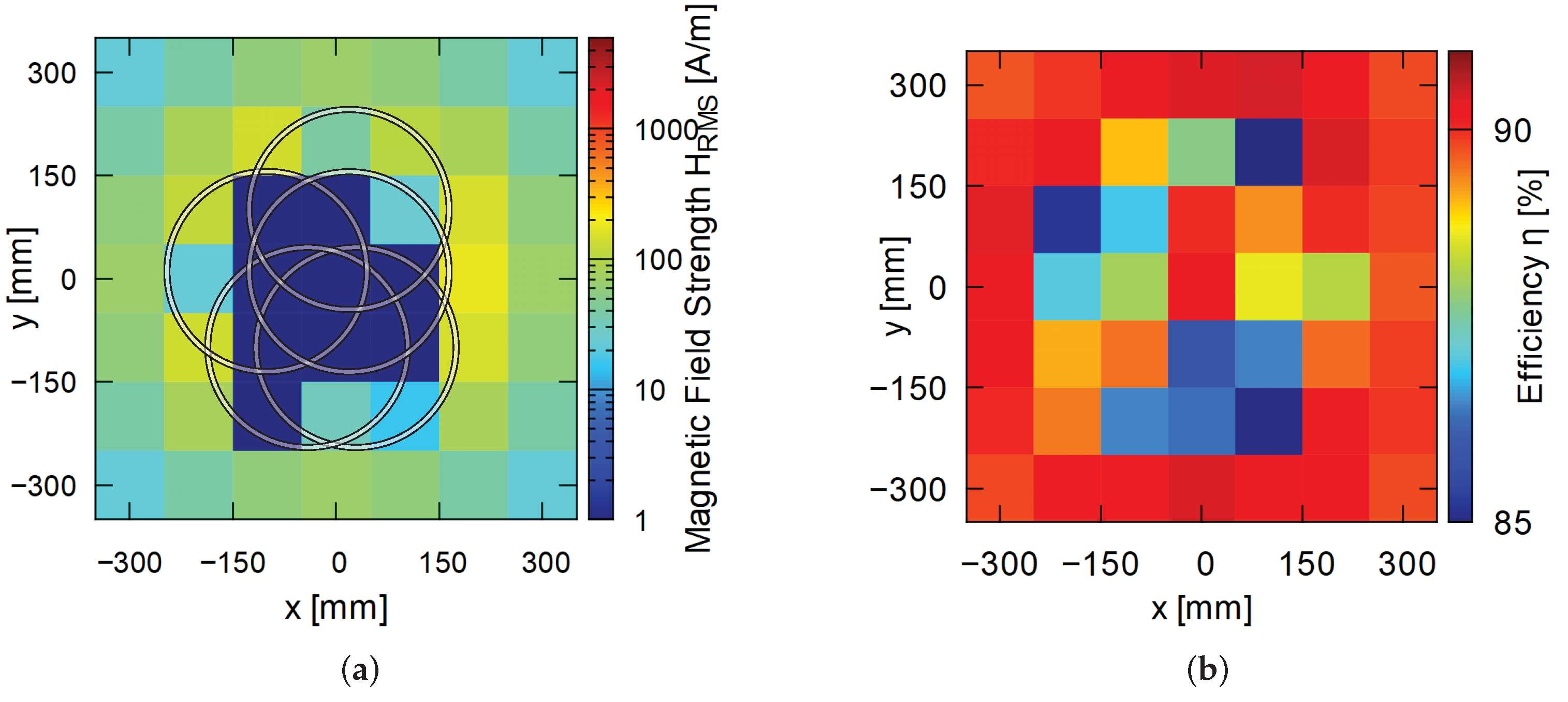
3.2. Simulation Results

A comparison of the magnetic field strength and transmission efficiency for each number of Tx coils at a field strength weight of $\alpha =0.1$, which prioritizes transmission efficiency, is shown in Figure 7. This figure compares the results with the optimal configuration for each number of Tx coils, as searched by PSO.

The red-line graph reveals that the maximum efficiency among all evaluation points increased slightly with the number of Tx coils from 90.2% with one Tx to 90.7% with five Tx coils. The results are consistent with those of previous studies [34,35,36,37,38,39]. The minimum efficiency value shown in the blue-line graph was higher than the lower efficiency limit ${\eta }_{limit}$ of 85%. In particular, it was greater than 89.3% for each number of Tx coils. In addition, the sum of the magnetic field strengths at all evaluation points indicated by the bar graph and the maximum value of the magnetic field strength indicated by the orange-line graph decreased inversely with the number of Tx coils. Compared with one Tx coil, the total magnetic field strength and the maximum strength were suppressed by 83.0% and 94.4%, respectively, with five Tx coils. These results indicate that the suppression effect was not negligible, thus confirming the effectiveness of the evaluation functions, namely, Equations (18) and (19).

Figure 8 presents a comparison of the magnetic field strength and efficiency for each number of Tx coils with a weight of $\alpha =0.9$, which gives priority to magnetic field suppression.

The maximum efficiency did not increase with the increase in the number of Tx coils. The minimum efficiency value was within with the lower efficiency limit ${\eta }_{limit}$ of 85%. The total magnetic field strength and the maximum magnetic field strength decreased as the number of Tx coils increased and the total magnetic field strength and maximum magnetic field strength were suppressed by 87.8% and 95.1%, respectively, with five Tx coils, when compared with one Tx coil. These results indicate that $\alpha =0.1$, which was superior for transmission efficiency, whereas $\alpha =0.9$, which was superior for magnetic field suppression. The difference in characteristics was the most significant when the number of Tx coils was the largest, with five Tx coils.

Figure 9 presents the influence of $\alpha$ on the transmission efficiency and the magnetic field suppression effect with five Tx coils, where the difference in characteristics was more significant; the total magnetic field strength, maximum transmission efficiency and minimum transmission efficiency at $\alpha =0.5$ were observed within the range $\alpha =0.1$–$0.9$.

Hence, the sum of the magnetic field strength, maximum transmission efficiency and minimum transmission efficiency decreased with the increase in the value of $\alpha$ and the characteristics changed in priority from efficiency to magnetic field suppression. However, the same trend was not observed for the maximum magnetic field strength. This is because the maximum magnetic field strength is not directly evaluated by Equations (18) and (19), which are evaluation functions.

Next, we focused on the evaluation points at which the magnetic field suppression effect was enhanced using a phased array Tx coil in reference to the color map of the magnetic field strength and transmission efficiency. Figure 10 presents a color map of the magnetic field strength and efficiency for a typical configuration (one Tx coil) with a single Tx coil and an opposing Rx coil.

Moreover, one Tx coil was found to have a significantly large magnetic field strength near the origin (located in the vicinity of the coil), with a value of 3.49 kA/m at four points where the strength was maximum. In contrast, a color map of the magnetic field strength and efficiency at $\alpha =0.9$ and five Tx coils, where the magnetic field suppression effect was greatest, is shown in Figure 11.

First, we explain how to read the color maps shown in Figure 10, Figure 11 and Figure 12. For example, with five Tx coils shown in Figure 11, the input voltage of the Tx coil with high magnetic field suppression effect at (0, 0, 10) mm, which is the evaluation point at the center of the evaluation plane, is as follows. For example, the phase and amplitude of the input voltage of each Tx coil with high magnetic field suppression effect at (0, 0, 10) mm, the evaluation point at the center of the evaluation plane for five Tx coils shown in Figure 11, are the values shown in the fifth row of

Table 4. Coordinates of evaluation points and transmission (Tx) coil arrangement and phase and amplitude of input voltage ($\alpha =0.9$, 5 Tx coils).

Coordinates of Evaluation Point (mm)	Transmission Efficiency $\mathit{\eta }$ (%)	Magnetic Field Strength ${\mathit{H}}_{\mathit{R}\mathit{M}\mathit{S}}$ (A/m)	Tx1 (mm) (30, −100, 0)		Tx2 (mm) (−40, −100, 0)		Tx3 (mm) (−100, 10, 0)		Tx4 (mm) (20, 100, 0)		Tx5 (mm) (20, 10, 0)
			Phase (Degree)	Amp (V)	Phase (Degree)	Amp (V)	Phase (Degree)	Amp (V)	Phase (Degree)	Amp (V)	Phase (Degree)	Amp (V)
(−200, 200, 10)	90.2	78.8	257.1	3094	247.8	3406	259.4	2956	239.5	2837	237.8	2712
(−200, 0, 10)	87.0	22.4	276.3	3842	128.1	202	304.6	3079	336.2	2715	277.2	3897
(−200, −200, 10)	89.4	76.6	184.0	3822	276.4	2055	196.3	3779	211.4	2686	209.0	2454
(0, 200, 10)	87.7	38.9	274.8	4446	252.0	1934	273.8	4546	222.9	2939	256.4	2097
(0, 0, 10)	90.3	5.0 × ${10}^{-6}$	224.3	1778	273.3	3473	246.1	2265	256.9	1557	250.3	4740
(0, −200, 10)	86.3	30.0	207.2	1346	296.5	1066	201.3	4166	320.7	46	236.0	5848
(200, 200, 10)	90.4	79.1	328.2	3248	336.0	3034	315.9	2491	325.3	2498	310.0	3451
(200, 0, 10)	88.2	170.3	320.3	3187	287.0	3880	278.7	2116	277.7	4799	359.9	2586
(200, −200, 10)	90.1	78.4	186.0	2107	124.6	3066	153.9	2011	144.7	2898	139.3	3320

. The magnetic field strength at the evaluation point was 5.0 $\times {10}^{-6}$ and the transmission efficiency was 90.3% when the power was transmitted with these optimal input voltages. Therefore, the center of the color map in Figure 11a is shown in blue and the center of the color map in Figure 11b is shown in red. As shown above, the color maps show the magnetic field strength and transmission efficiency of the optimized Tx coil configuration when wireless power transfer was performed at the optimum input voltage with a high magnetic field suppression effect at each evaluation point.

Here, the magnetic field strength near the origin, where the field strength was particularly large with one Tx coil, could be significantly suppressed while maintaining an efficiency of more than 85%. This indicates that the magnetic field strength at the evaluation point directly below the Rx coil can be significantly suppressed.

Finally, the input voltage values suitable for suppressing the magnetic field at each evaluation point were selected. Nine points at intervals of 200 mm in each x- and y-direction centered at the origin were chosen as representative points among the 49 points for coil arrangement and the phase and amplitude of the input voltage at those points are shown in Table 4.

Different combinations of the phase and amplitude were selected for each evaluation point.

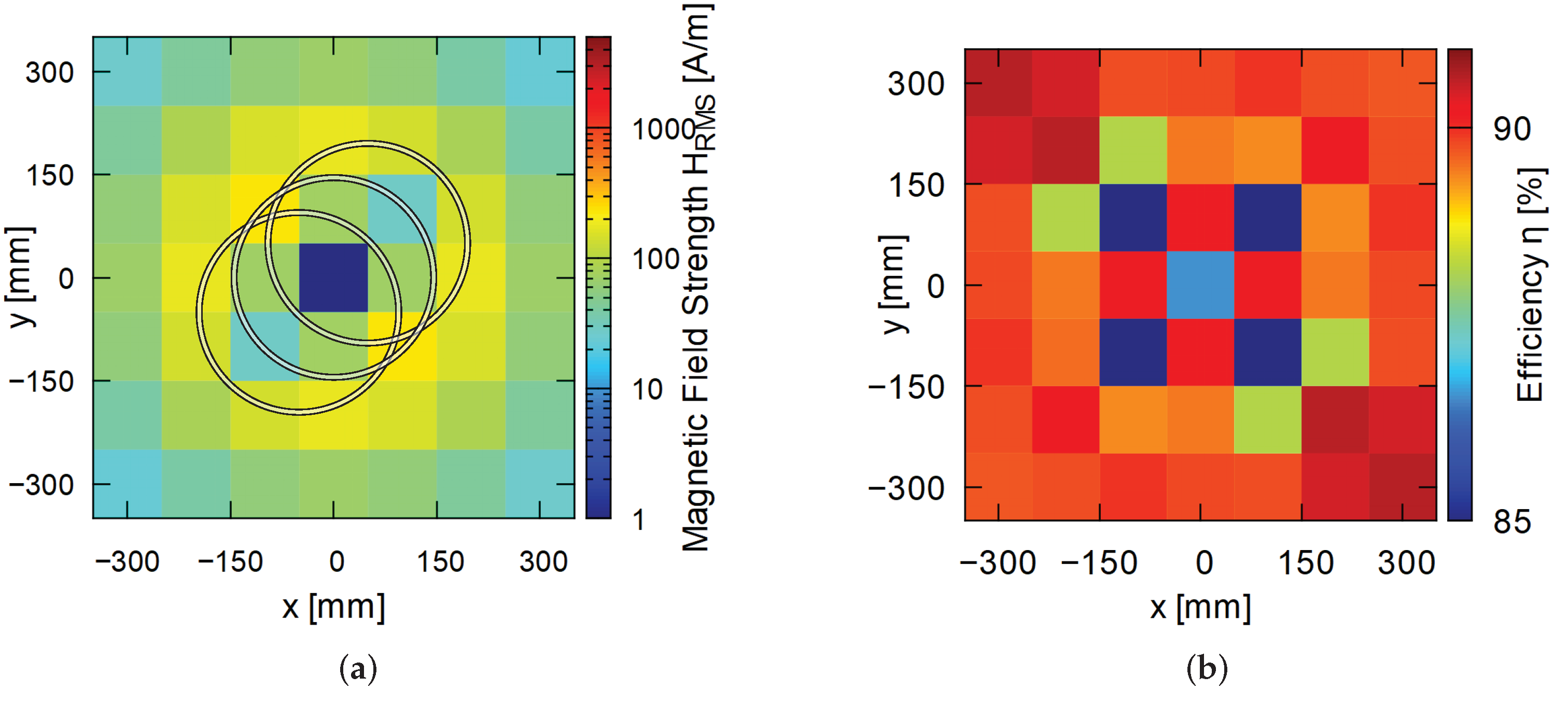
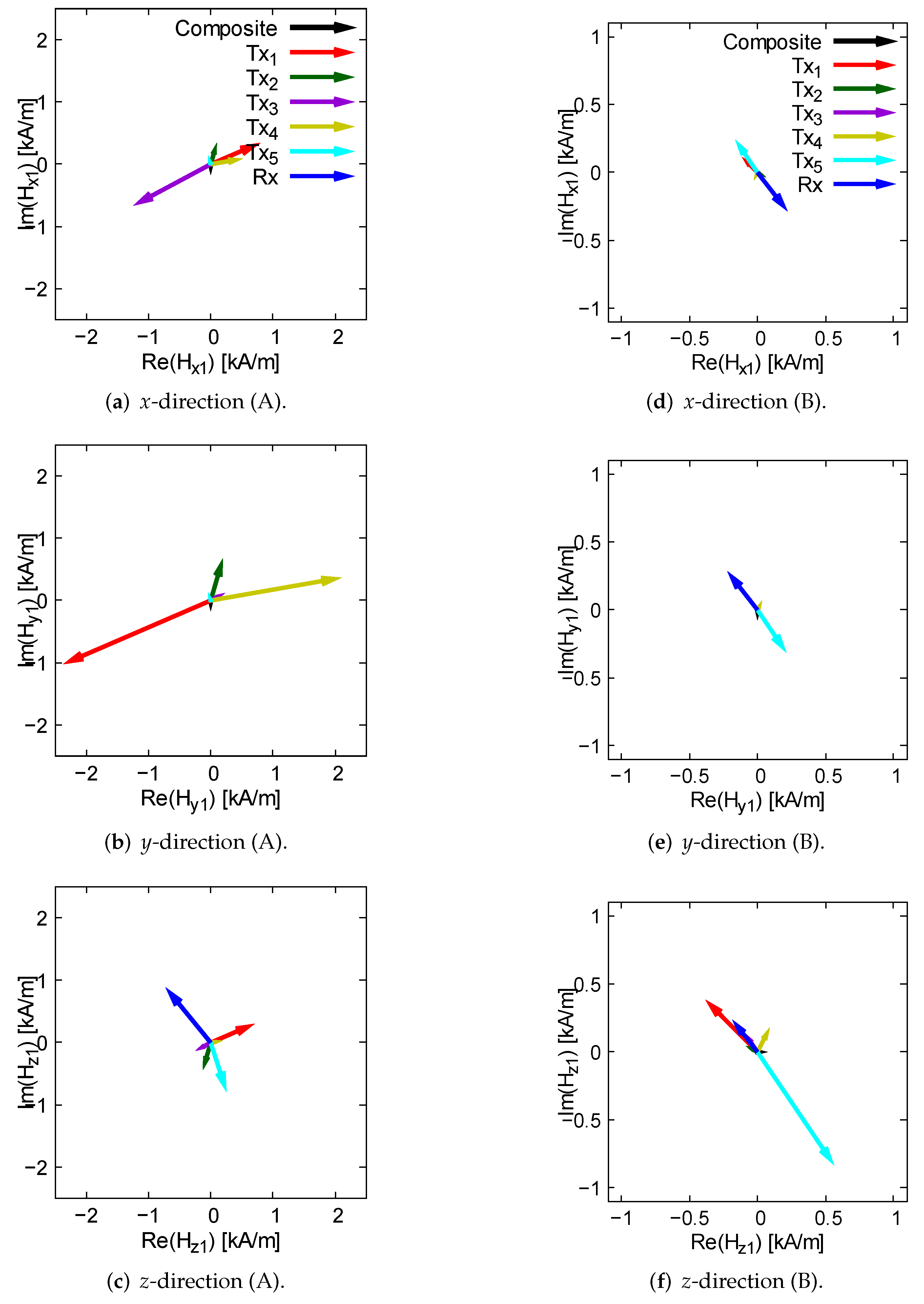
3.3. State of Magnetic Field Suppression

This section discusses the magnetic field suppression effect for two representative evaluation points in each coil arrangement of different numbers of Tx coils.

As mentioned previously, the magnetic field suppression effect was found to improve as the number of Tx coils increased. This section discusses and focuses on two specific evaluation points to examine changes in the behavior of the field generated by each coil and its associated composite field with an increase in the number of coils. The color maps of the magnetic field strength and efficiency for three Tx coils ($\alpha =0.9$) are shown in Figure 12.

To examine the step-wise improvement of the magnetic field suppression effect between three Tx and five Tx coils, we selected two points such that only one of the points was sufficiently suppressed with three Tx coils and both points were sufficiently suppressed with five Tx coils. Here, the evaluation points A (0, 0, 10) mm and B (100, −100, 10) mm were selected by referring to Figure 11 and Figure 12. With three Tx coils, only the magnetic field of A was suppressed and, with five Tx coils, the magnetic fields of both A and B were suppressed.

Here, we focus on each component of the magnetic field, i.e., the magnetic field generated by each coil displayed as a phasor, as well as their composite vector.

The phasor display of each component of the magnetic field with three Tx coils is shown in Figure 13.

Figure 13a–f presents the phasor display of the each component of magnetic field at A and B. The composite vector is the combination of vectors generated by all coils. Hence, with a decrease in the norm of this vector, it could be said that the magnetic field suppression increased in that direction. The phasor diagram presented in this paper is for time $t=0$, which corresponds to the state of $k=1$ in Equations (10)–(12). As k increased, all vectors were rotated counterclockwise without changing their lengths. Figure 13a–c confirms that the composite vector was significantly small in each direction, which shows that the magnetic field suppression effect was high at A.

At A, the input power to each Tx coil was ${\mathrm{Tx}}_1=-944$ W, ${\mathrm{Tx}}_2=-944$ W and ${\mathrm{Tx}}_3=14,596$ W. This indicates that ${\mathrm{Tx}}_3$ contributed the most to the power transmission to Rx and that ${\mathrm{Tx}}_1$ and ${\mathrm{Tx}}_2$ worked to suppress the magnetic field. The negative power of ${\mathrm{Tx}}_1$ and ${\mathrm{Tx}}_2$ acted as the regenerative energy. Given that the x–y coordinates of ${\mathrm{Tx}}_3$ and Rx were $x=y=0$, which were the same for point A, the vectors generated in the x- and y-directions by ${\mathrm{Tx}}_3$ and Rx were zero vectors. The phases and amplitudes of the input voltages and currents of ${\mathrm{Tx}}_1$ and ${\mathrm{Tx}}_2$ were completely matched; therefore, vectors generated by ${\mathrm{Tx}}_1$ and ${\mathrm{Tx}}_2$ canceled each other in the x- and y-direction as shown in Figure 13a,b and generated the same vector in the z-direction as shown in Figure 13c, to eliminate the vectors generated by ${\mathrm{Tx}}_3$ and Rx.

At B, the input power to each Tx coil was ${\mathrm{Tx}}_1=26,045$ W, ${\mathrm{Tx}}_2=26,196$ W and ${\mathrm{Tx}}_3=-39,299$ W. This suggests that ${\mathrm{Tx}}_1$ and ${\mathrm{Tx}}_2$ contributed to the power transmission to Rx and that only ${\mathrm{Tx}}_3$ worked to suppress the magnetic field. Hence, Figure 13d–f reveals that the vector of ${\mathrm{Tx}}_3$ was at an angle close to the opposite direction of the composite vectors of Rx, ${\mathrm{Tx}}_1$ and ${\mathrm{Tx}}_2$. However, the composite vector remained, because the magnetic field vectors did not cancel each other, which may be because only a single coil worked to suppress the magnetic field. Same as in the case in Figure 13c, ${\mathrm{Tx}}_1$ and ${\mathrm{Tx}}_2$ generated almost identical vectors in the z-direction.

The phasor display of the magnetic field in each direction with five Tx coils is shown in Figure 14.

The composite vector in each direction became almost zero at not only A, where the magnetic field suppression effect was high with three Tx coils, but also at B, where the magnetic field suppression effect was insufficient with three Tx coils.

The power input to each Tx coil at B was ${\mathrm{Tx}}_1=79$ W, ${\mathrm{Tx}}_2=-216$ W, ${\mathrm{Tx}}_3=11,191$ W, ${\mathrm{Tx}}_4=24,243$ W and ${\mathrm{Tx}}_5=-22,575$ W. This indicates that ${\mathrm{Tx}}_3$ and ${\mathrm{Tx}}_4$ mainly contributed to the power transmission. However, since these coils were located a distance away from B, they had little effect on the magnetic field in each direction, as shown in Figure 14d–f. Therefore, ${\mathrm{Tx}}_3$ and ${\mathrm{Tx}}_4$ were mainly used for power transmission; the other three Tx coils, including Rx, were mainly used for magnetic field suppression. Compared with three Tx coils, the number of coils that could be used mainly for magnetic field suppression increased, thus leading to a more effective suppression. Here, the vectors generated by Rx in Figure 14a,b and the ${\mathrm{Tx}}_1$ and ${\mathrm{Tx}}_2$ in Figure 14e were zero vectors and the other vectors were non-zero, although several were difficult to recognize due to their small size.

4. Conclusions

In this paper, we propose a novel WPT function for EVs in parking lots, which enables continuous high-efficiency WPT while minimizing magnetic field absorption by metallic foreign objects. In this study, this issue was considered as a problem where a metallic foreign object is present at an arbitrary point in a two-dimensional plane and the solution was investigated assuming the usage of phased array WPT. A searching algorithm using PSO is proposed to search for the optimal coil configuration and the optimal input voltage of each coil for each magnetic field suppression position in that coil configuration.

The simulation results show the following. First, an increase in the number of Tx coils contributed significantly to the improvement of the magnetic field suppression effect and, with five Tx coils, the magnetic field suppression effect improved significantly compared to one Tx coil. Here, for the same number of Tx coils, the simulation parameter $\alpha$, which corresponds to the weight factor of transmission efficiency and magnetic field suppression in the evaluation function, functioned appropriately due to the fact that the transmission efficiency increased when given priority and vice versa in case of the magnetic field suppression.

Next, by analyzing the phasor display of the magnetic field in each direction, it was found that using a large number of Tx coils led to utilizing Tx coils for different main purposes, such as power transmission and magnetic field suppression, depending on the evaluation point, which contributed to both maintaining efficiency and improving the magnetic field suppression effect. In addition, it should be noted that a transmission efficiency of more than 85% was maintained in all simulations.

In the proof-of-principle stage, it was confirmed that the proposed method of high efficiency WPT with magnetic field suppression was possible for at least a single point

We consider the following as possible future works. The development of a control circuit to share the single power supply would be expected, because, currently, each Tx coil requires a separate inverter. Since there are cases where more than one metal object is scattered, we would like to continue to study the effect of magnetic field suppression in the case of two or more points. Furthermore, we would like to consider suppression not only by points but also by shapes, such as lines. Finally, we would like to conduct simulations and actual experiments considering the influence of power electronic converters.

References

1. Un-Noor, F.; Padmanaban, S.; Mihet-Popa, L.N.; Mollah, M.; Hossain, E. A Comprehensive Study of Key Electric Vehicle (EV) Components, Technologies, Challenges, Impacts, and Future Direction of Development. Energies 2017, 10, 1217. [Google Scholar] [CrossRef] [Green Version]
2. Kurs, A.; Karalis, A.; Moffatt, R.; Joahannopoulos, J.D.; Fisher, P.; Soljačić, M. Wireless Power Transfer via Strongly Coupled Magnetic Resonances. Science 2007, 317, 83–86. [Google Scholar] [CrossRef] [PubMed] [Green Version]
3. Li, S.; Mi, C.C. Wireless Power Transfer for Electric Vehicle Applications. IEEE J. Emerg. Sel. Top. Power Electron. 2015, 3, 4–17. [Google Scholar]
4. Mou, X.; Groling, O.; Sun, H. Energy-Efficient and Adaptive Design for Wireless Power Transfer in Electric Vehicles. IEEE Trans. Ind. Electron. 2017, 64, 7250–7260. [Google Scholar] [CrossRef] [Green Version]
5. Qiu, C.; Chau, K.T.; Liu, C.; Chan, C.C. Overview of wireless power transfer for electric vehicle charging. Proc. Electr. Veh. Symp. Exhib. (EVS) 2013, 7, 1–9. [Google Scholar]
6. Yokoi, Y.; Taniya, A.; Horiuchi, M.; Kobayashi, S. Development of kW class wireless power transmission system for EV using magnetic resonant method. SAE Tech. Pap. 2011, 2011-39-7267. [Google Scholar]
7. Standard SAE J2954. Wireless Power Transfer for Light-Duty Plug-In/Electric Vehicles and Alignment Methodology. 2020. Available online: https://www.sae.org/standards/content/j2954_202010/ (accessed on 31 December 2021).
8. Ahmad, A.; Alam, M.; Rafat, Y.; Shariff, S.; Al-Saidan, I.; Chabaan, R. Foreign Object Debris Detection and Automatic Elimination for Autonomous Electric Vehicles Wireless Charging Application. SAE Int. J. Elec. Veh. 2020, 9, 93–110. [Google Scholar] [CrossRef]
9. Zhang, Y.; Yan, Z.; Zhu, J.; Li, S.; Mi, C. A review of foreign object detection (FOD) for inductive power transfer systems. eTransportation 2019, 1, 100002. [Google Scholar] [CrossRef]
10. Xiang, L.; Zhu, Z.; Tian, J.; Tian, Y. Foreign Object Detection in a Wireless Power Transfer System Using Symmetrical Coil Sets. IEEE Access 2019, 7, 44622–44631. [Google Scholar] [CrossRef]
11. Ombach, G. Design and safety considerations of interoperable wireless charging system for automotive. In Proceedings of the 9th International Conference on Ecological Vehicles and Renewable Energies (EVER), Monte-Carlo, Monaco, 25–27 March 2014; pp. 1–4. [Google Scholar]
12. Sonnenberg, T.; Stevens, A.; Dayerizadeh, A.; Lukic, S. Combined Foreign Object Detection and Live Object Protection in Wireless Power Transfer Systems via Real-Time Thermal Camera Analysis. In Proceedings of the IEEE Applied Power Electronics Conference and Exposition (APEC), Anaheim, CA, USA, 17–21 March 2019; pp. 1547–1552. [Google Scholar]
13. Liu, X.; Liu, C.; Han, W.; Pong, P.W.T. Design and Implementation of a Multi-Purpose TMR Sensor Matrix for Wireless Electric Vehicle Charging. IEEE Sens. J. 2019, 19, 1683–1692. [Google Scholar] [CrossRef]
14. Refence Designs. Available online: https://witricity.com/products/reference-designs/ (accessed on 25 December 2021).
15. D-Broad, EV. Available online: https://www.daihen.co.jp/products/wireless/ev/ (accessed on 25 December 2021).
16. Dobrzański, D. Overview of currently used wireless electrical vehicle charging solutions. IAPGOS 2018, 8, 47–50. [Google Scholar] [CrossRef]
17. Lim, Y.; Park, J. A Novel Phase-Control-Based Energy Beamforming Techniques in Nonradiative Wireless Power Transfer. IEEE Trans. Power Electron. 2015, 30, 6274–6287. [Google Scholar] [CrossRef]
18. Zhu, Q.; Su, M.; Sun, Y.; Tang, W.; Hu, A.P. Field Orientation Based on Current Amplitude and Phase Angle Control for Wireless Power Transfer. IEEE Trans. Ind. Electron. 2018, 65, 4758–4770. [Google Scholar] [CrossRef]
19. Kim, K.; Kim, H.-J.; Seo, D.-W.; Choi, J.-W. Analysis on Influences of Intra-Couplings in a MISO Magnetic Beamforming Wireless Power Transfer System. Energies 2021, 14, 5184. [Google Scholar] [CrossRef]
20. Ming, C.; Yanting, L.; Yongmin, Y.; Yingchun, Z.; Yingxiao, X. Performance Optimization Method of Wireless Power Transfer System Based on Magnetic Field Editing. In Proceedings of the 4th International Conference on Advanced Electronic MaterialsInternational Conference on Advanced Electronic Materials, Computers and Software Engineering (AEMCSE), Changsha, China, 26–28 March 2021; pp. 10–17. [Google Scholar]
21. Waters, B.H.; Mahoney, B.J.; Ranganathan, V.; Smith, J.R. Power Delivery and Leakage Field Control Using an Adaptive Phased Array Wireless Power System. IEEE Trans. Power Electron. 2015, 30, 6298–6309. [Google Scholar] [CrossRef]
22. Choi, B.; Park, B.; Lee, J. Near-Field Beamforming Loop Array for Selective Wireless Power Transfer. IEEE Microw. Compon. Lett. 2015, 25, 748–750. [Google Scholar] [CrossRef]
23. Sun, H.; Lin, H.; Zhu, F.; Gao, F. Magnetic Resonant Beamforming for Secured Wireless Power Transfer. IEEE Signal Process. Lett. 2017, 24, 1173–1177. [Google Scholar] [CrossRef]
24. Tian, X.; Chau, K.T.; Liu, W.; Lee, C.H.T. Selective Wireless Power Transfer Using Magnetic Field Editing. IEEE Trans. Power Electron. 2021, 36, 2710–2719. [Google Scholar] [CrossRef]
25. Pasku, V.; De Angelis, A.; Dionigi, M.; Moschitta, A.; De Angelis, G.; Carbone, P. Analysis of Nonideal Effects and Performance in Magnetic Positioning Systems. IEEE Trans. Instrum. Meas. 2016, 65, 2816–2827. [Google Scholar] [CrossRef]
26. Pasku, V.; De Angelis, A.; Dionigi, M.; De Angelis, G. A Positioning System Based on Low-Frequency Magnetic Fields. IEEE Trans. Ind. Electron. 2016, 63, 2457–2468. [Google Scholar] [CrossRef]
27. Nakamura, S.; Hashimoto, H. Error Characteristics of Passive Position Sensing via Coupled Magnetic Resonances Assuming Simultaneous Realization With Wireless Charging. IEEE Sens. J. 2015, 15, 3675–3686. [Google Scholar] [CrossRef]
28. Nakamura, S.; Namiki, M.; Sugimoto, Y.; Hashimoto, H. Q Controllable Antenna as a Potential Means for Wide-Area Sensing and Communication in Wireless Charging via Coupled Magnetic Resonances. IEEE Trans. Power Electron. 2017, 32, 218–232. [Google Scholar] [CrossRef]
29. Zhang, B.; Chen, Q.; Ke, G.; Xu, L.; Ren, X.; Zhang, Z. Coil Positioning Based on DC Pre-excitation and Magnetic Sensing for Wireless Electric Vehicle Charging. IEEE Trans. Ind. Electron. 2021, 68, 3820–3830. [Google Scholar] [CrossRef]
30. Kennedy, J.; Eberhart, R. Particle swarm optimization. Proc. IEEE Int. Conf. Neural Netw. 1995, 4, 1942–1948. [Google Scholar]
31. Akatsu, K. Available online: https://www.shibaura-it.ac.jp/albums/abm.php?d=429&f=abm00002401.pdf (accessed on 31 December 2021).
32. Nikkei Electronics. Available online: https://xtech.nikkei.com/atcl/nxt/mag/ne/18/00007/00148/?P=5 (accessed on 31 December 2021).
33. Zaheer, A.; Covic, G.A.; Kacprzak, D. A Bipolar Pad in a 10-kHz 300-W Distributed IPT System for AGV Applications. IEEE Trans. Ind. Electron. 2014, 61, 3288–3301. [Google Scholar] [CrossRef]
34. Oodachi, N.; Ogawa, K.; Kudo, H.; Shoki, H.; Obayashi, S. Efficiency Improvement of Wireless Power Transfer Via Magnetic Resonance Using Transmission Coil Array. In Proceedings of the IEEE International Symposium on Antennas and Propagation (APSURSI), Spokane, WA, USA, 3–8 July 2011; pp. 1707–1710. [Google Scholar]
35. Zhong, W.X.; Zhang, C.; Liu, X.; Hui, S.Y.R. A Methodology for Making a Three-Coil Wireless Power Transfer System More Energy Efficient Than a Two-Coil Counterpart for Extended Transfer Distance. IEEE Trans. Power Electron. 2015, 30, 933–942. [Google Scholar] [CrossRef]
36. Lang, H.; Ludwig, A.; Sarris, C.D. Convex Optimization of Wireless Power Transfer Systems With Multiple Transmitters. IEEE Trans. Antenna Propag. 2014, 62, 4623–4636. [Google Scholar] [CrossRef]
37. Yang, G.; Vedady Moghadam, M.R.; Zhang, R. Magnetic beamforming for wireless power transfer. In Proceedings of the IEEE International Conference on Acoustics, Speech and Signal Processing (ICASSP), Shanghai, China, 20–25 March 2016; pp. 3936–3940. [Google Scholar]
38. Huang, Y.; Liu, C.; Liu, S.; Xiao, Y. A Selectable Regional Charging Platform for Wireless Power Transfer. In Proceedings of the 45th Annual Conference of the IEEE Industrial Electronics Society, Lisbon, Portugal, 14–17 October 2019; pp. 4445–4450. [Google Scholar]
39. Hamano, K.; Ohtsuka, K.; Tanaka, R.; Nishikawa, K. 4×1 Multi-Input Single-Output Magnetic Resonance Beamforming Wireless Power Transfer System. In Proceedings of the International Applied Computational Electromagnetics Society Symposium (ACES), Suzhou, China, 1–4 August 2017; pp. 1–2. [Google Scholar]
Figure 1. Simplified image of magnetic field distribution and flowchart.
Energies 15 01028 g001
Figure 2. Equivalent circuit of wireless power transfer via magnetic resonance coupling (MRC-WPT) using phased array transmission (Tx) coils. Since the magnetic field at the position of the interfering object was assumed to be suppressed, their effect was ignored (approximation).
Energies 15 01028 g002
Figure 3. The magnetic field strength at the calculation point generated by each coil. It is calculated as the composite of the magnetic fields generated by all of the coils.
Energies 15 01028 g003
Figure 4. Transmission (Tx) coil configuration plane.
Energies 15 01028 g004
Figure 5. Evaluation points in the evaluation plane.
Energies 15 01028 g005
Figure 6. Flowchart of the optimization process using particle swarm optimization (PSO). This simulation program has a double-loop structure that consists of the optimization of the coil configuration and that of the phase and amplitude of the input voltage to each coil at each evaluation point in the evaluation plane.
Energies 15 01028 g006
Figure 7. Comparison of magnetic field strength and transmission efficiency for each number of transmission (Tx) coils ( α = 0.1 ).
Energies 15 01028 g007
Figure 8. Comparison of magnetic field strength and transmission efficiency for each number of transmission (Tx) coils ( α = 0.9 ).
Energies 15 01028 g008
Figure 9. Effect of magnetic field strength weight α on the transmission efficiency and magnetic field suppression for 5 Tx.
Energies 15 01028 g009
Figure 10. Color map (1 Tx): (a) transmission (Tx) coil configuration and magnetic field strength map and (b) transmission efficiency map. At the evaluation point (center of each cell), with the decrease in the magnetic field strength H R M S , the blue shading in the cell becomes darker and, with the increase in the power transmission efficiency η , the red shading in the cell becomes darker.
Energies 15 01028 g010
Figure 11. Color map ( α = 0.9 , 5 Tx coils): (a) transmission (Tx) coil configuration and magnetic field strength map and (b) transmission efficiency map. The Tx coil configuration was as follows: Tx 1 , (30, −100, 0) mm; Tx 2 , (−40, −100, 0) mm; Tx 3 , (−100, 10, 0) mm; Tx 4 , (20, 100, 0) mm; Tx 5 , (20, 10, 0) mm.
Energies 15 01028 g011
Figure 12. Color map ( α = 0.9 , 3 Tx coils): (a) transmission (Tx) coil configuration and magnetic field strength map and (b) transmission efficiency map. The Tx coil configuration was as follows: Tx 1 , (−50, −50, 0) mm; Tx 2 , (50, 50, 0) mm; Tx 3 , (0, 0, 0) mm.
Energies 15 01028 g012
Figure 13. Phasor representation of the magnetic field in each direction ( α = 0.9 , three Tx coils, k = 1 ): (ac) magnetic field at A; (df) magnetic field at B.
Energies 15 01028 g013
Figure 14. Phasor representation of the magnetic field in each direction ( α = 0.9 , five Tx coils, k = 1 ): (ac) magnetic field at A; (df) magnetic field at B.
Energies 15 01028 g014