
Will Capacity Mechanisms Conflict with Carbon Pricing? †


Abstract
1. Introduction
2. Methodology and Data Sources
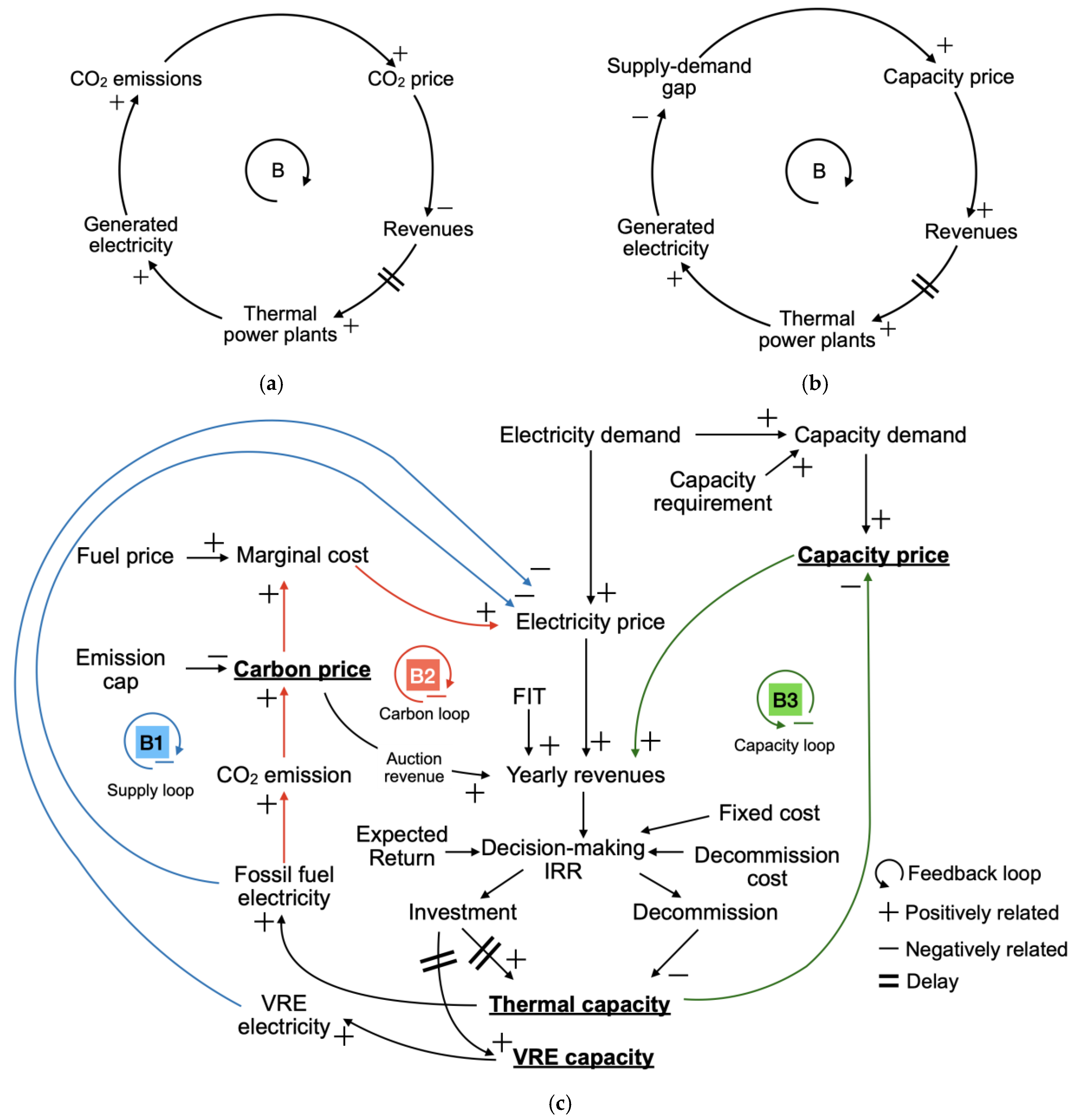
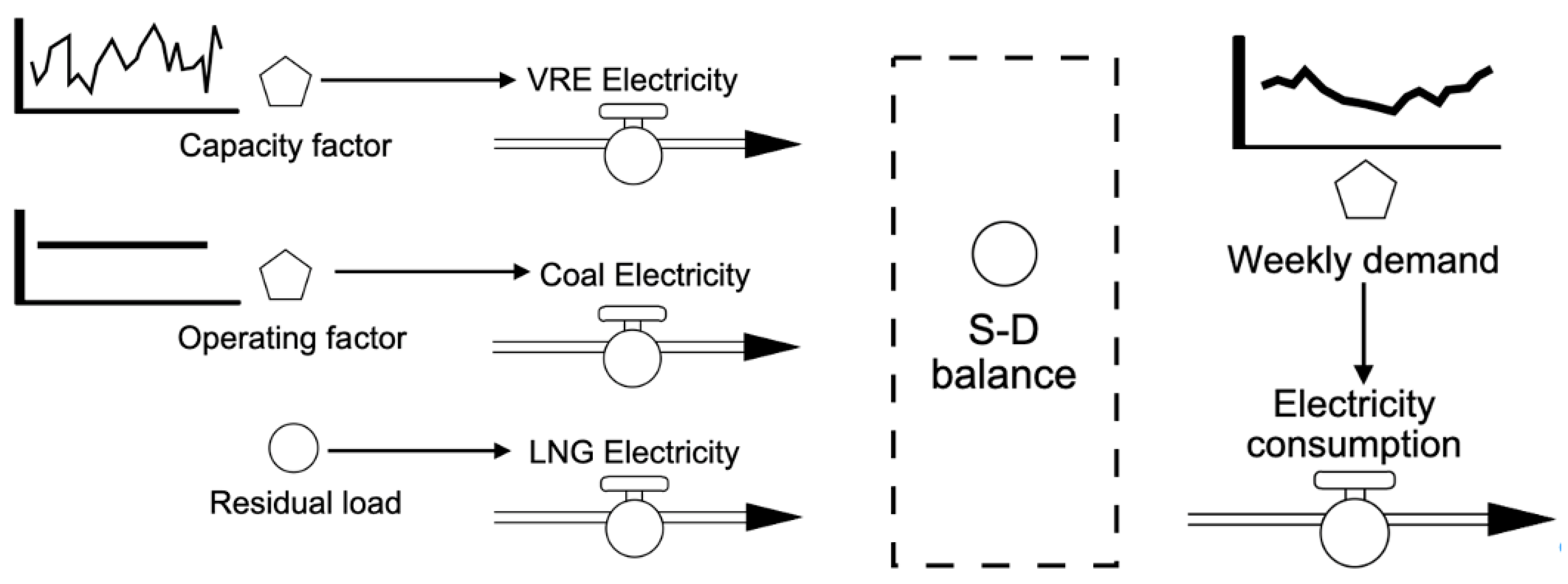
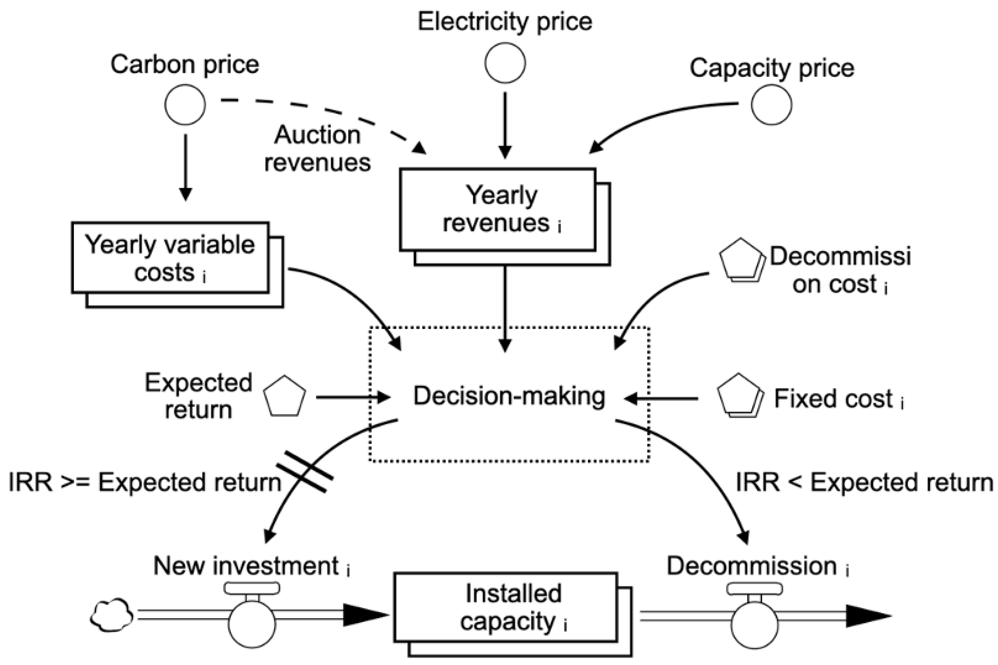
2.1. Conceptual Model as the Framework
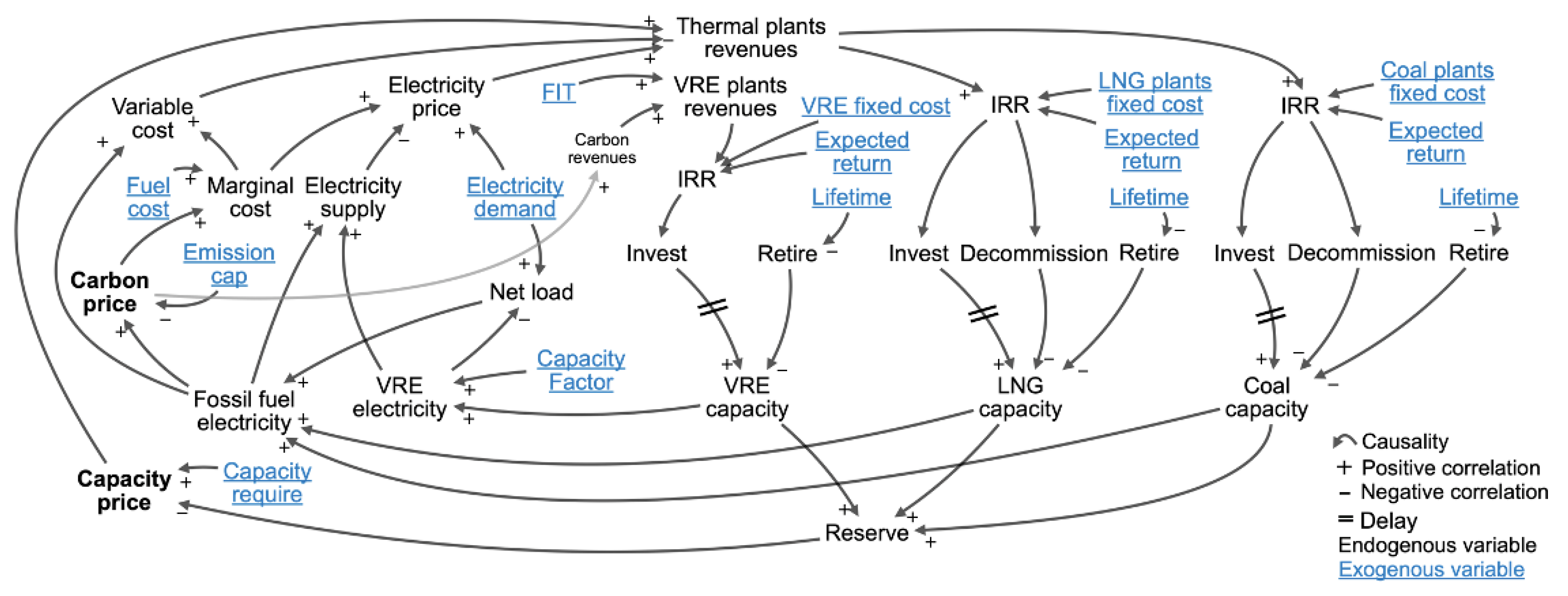
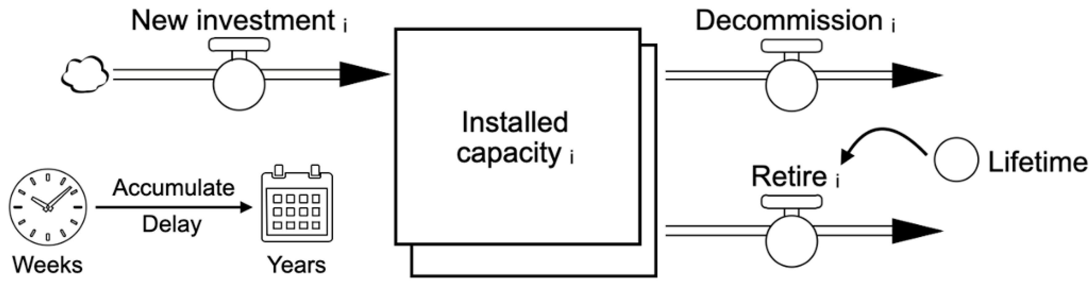
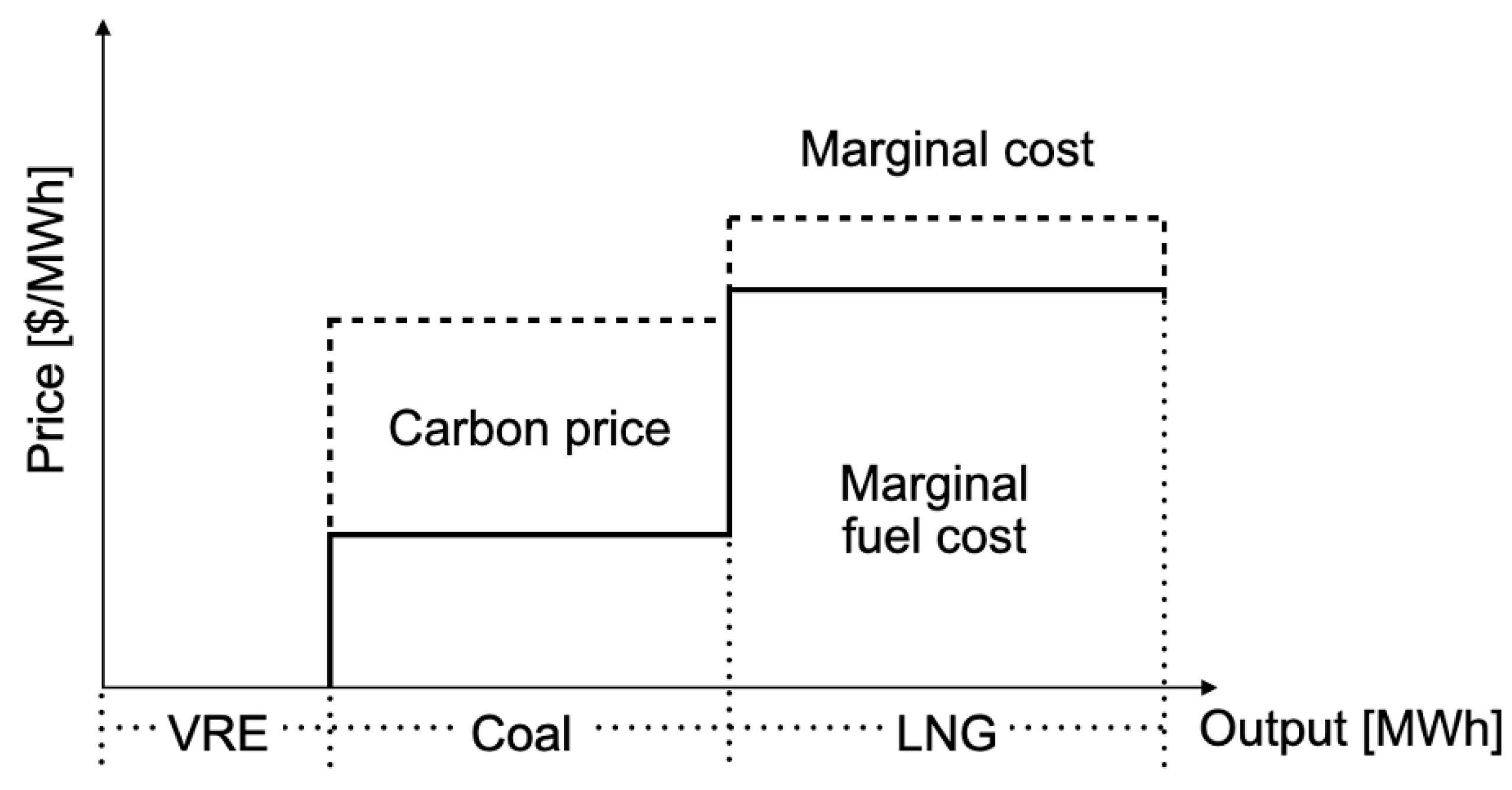
2.2. Quantitative Model Formulation
| (11) | |||
| - |
2.3. Case Study
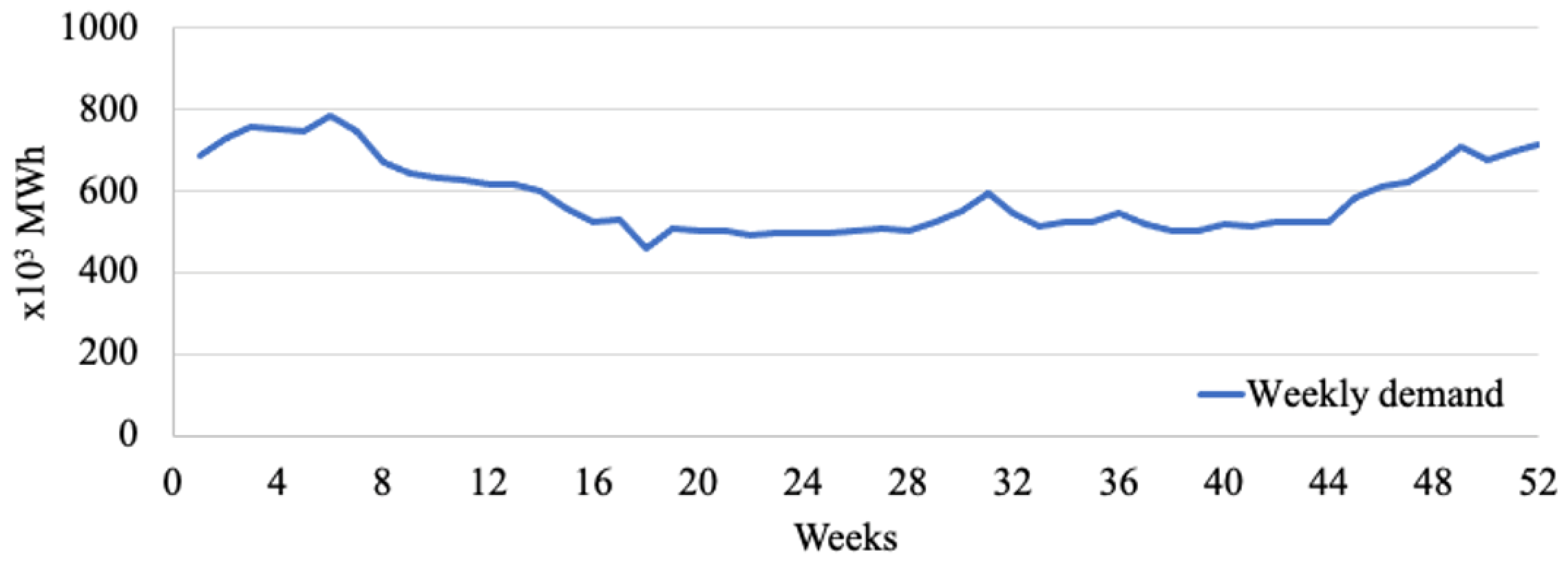
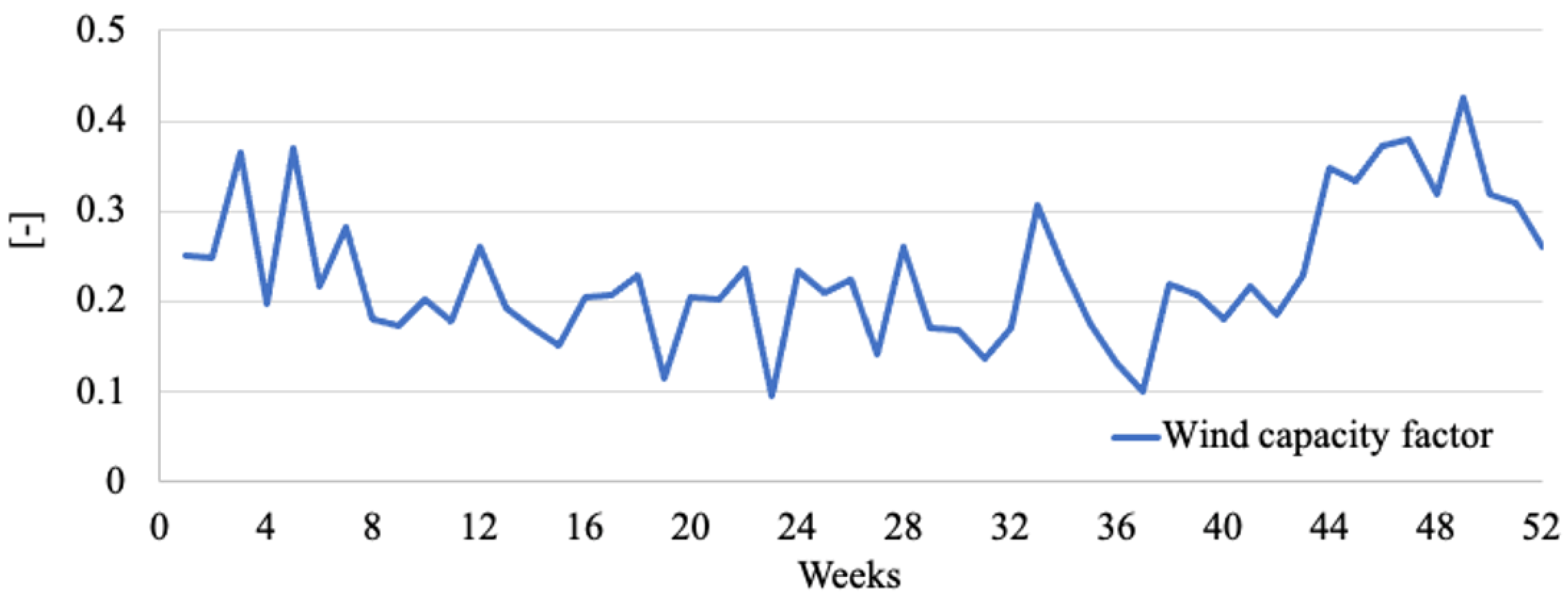
2.4. Data Sources

| Variables (Unit) | Wind | Coal | NG |
|---|---|---|---|
| Initial capacity (MW) | 534 | 2520 | 3507 |
| Minimum size of generators set 1 (MW) | 5 | 100 | 200 |
| Construction time (yr) | 1 | 3 | 3 |
| Investment coefficient (-) | 40 | 1 | 1 |
| Decommissioning coefficient (-) | - | 1 | 1 |
| Wind capacity value factor (-) | 0.236 | 1 | 1 |
| Mean Fuel Price in 2019 (USD/ton) | - | 108.58 | 512.99 |
| Marginal Fuel Cost (USD/MWh) | - | 35.84 | 67.14 |
| Emission Factor (ton-CO2/MWh) | - | 0.943 | 0.474 |
| Heat value (MJ/ton) | - | 25,970 | 55,010 |
| Heat efficiency (-) | - | 0.42 | 0.5 |
| Fixed cost (USD/MW) | 2,590,476 | 2,380,952 | 1,142,857 |
| Maintenance cost (USD/MW/yr) | 2590 | 119,047 | 57,142 |
| Decommission cost ratio (-) | 0.01 | 0.07 | 0.07 |
| Lifetime (yr) | 20 | 40 | 40 |
| Interest rate (-) | 0.03 | ||
| Sensitivity coefficient of carbon price | 1 | ||
| Sensitivity coefficient of capacity price | 130,725.8 * | ||
| Sensitivity coefficient of electricity price | 10 | ||
| FIT (USD/MWh) | 95 | ||
| CO2 floor price (USD/ton-CO2) | 30 | ||
| Capacity price cap (USD/MW) | 134,647.6 ** | ||
| Electricity price cap (USD/MWh) | 1905 | ||
| Exchange rate (JPY/USD) | 105 | ||
3. Results and Discussion
3.1. Scenario Setting
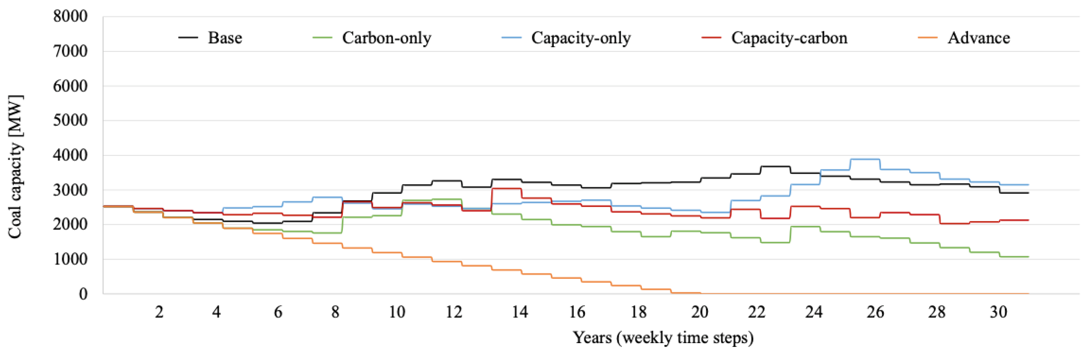
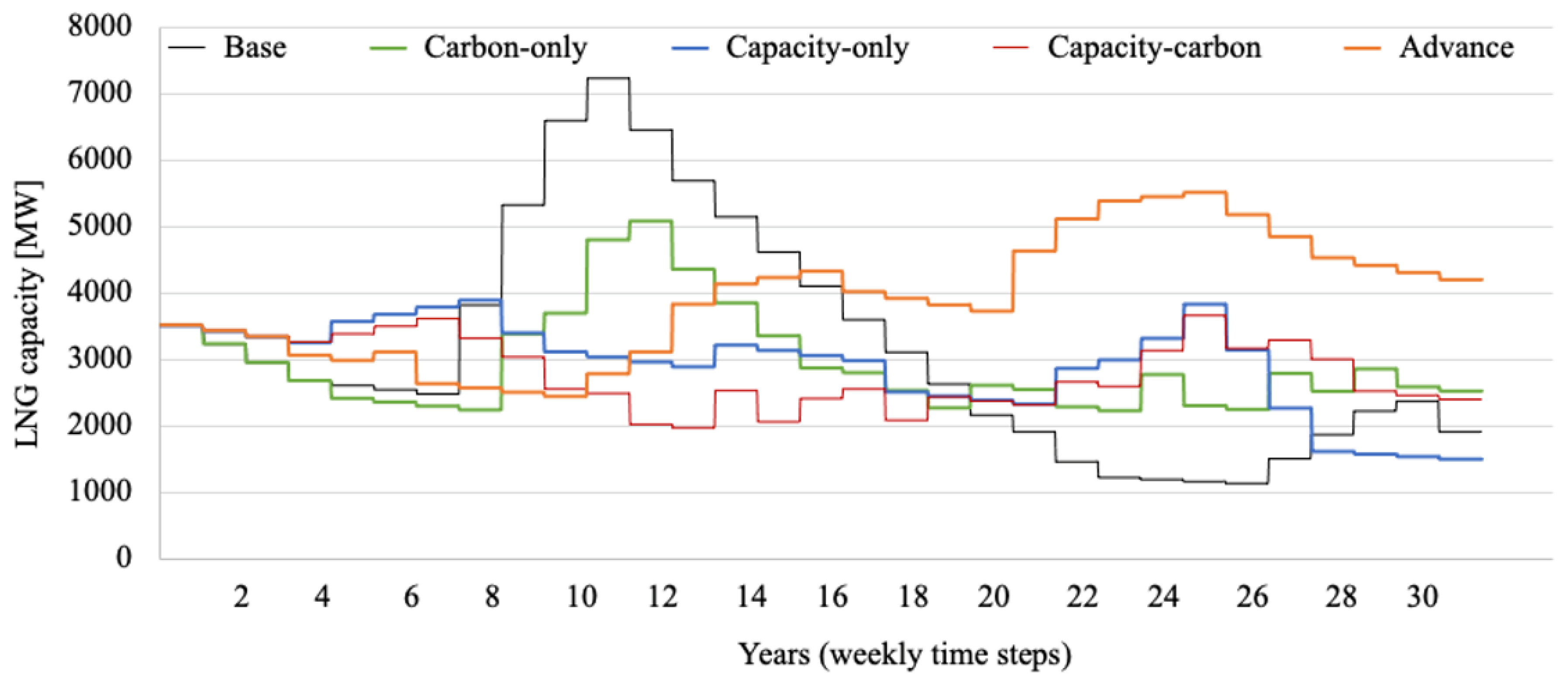
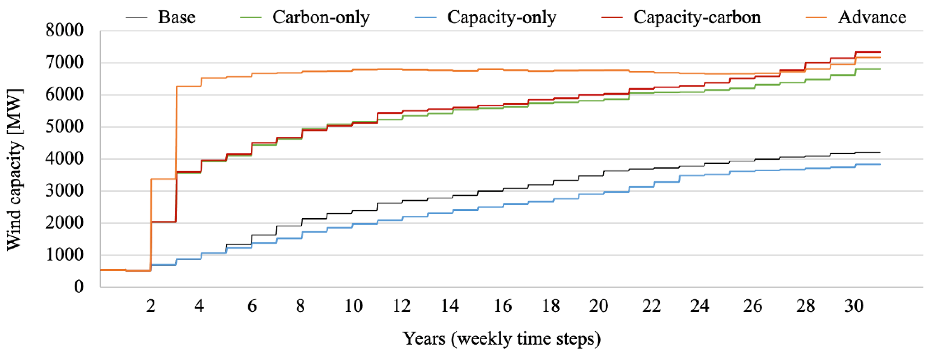
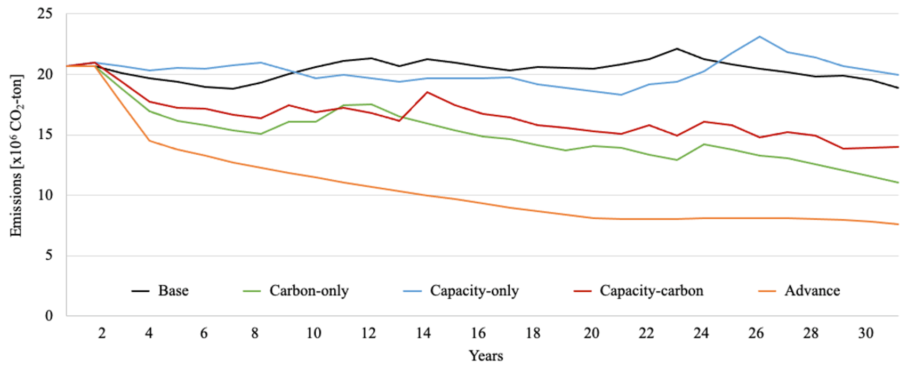
3.2. Simulation Results
3.3. Policy Implications
4. Conclusions
Author Contributions
Funding
Data Availability Statement
Conflicts of Interest
References
- Quéré, C.; Andrew, R.M.; Friedlingstein, P.; Sitch, S.; Hauck, J.; Pongratz, J.; Pickers, P.A.; Korsbakken, J.I.; Peters, G.P.; Canadell, J.G.; et al. Global carbon budget 2018. Earth Syst. Sci. Data 2018, 10, 2141–2194. [Google Scholar] [CrossRef]
- Peters, G.P.; Le Quéré, C.; Andrew, R.M.; Canadell, J.G.; Friedlingstein, P.; Ilyina, T.; Jackson, R.B.; Joos, F.; Korsbakken, J.I.; McKinley, C.A.; et al. Towards real-time verification of CO2 emissions. Nat. Clim. Chang. 2017, 7, 848–850. [Google Scholar] [CrossRef]
- Wilson, I.A.; Staffell, I. Rapid fuel switching from coal to natural gas through effective carbon pricing. Nat. Energy 2018, 3, 365–372. [Google Scholar] [CrossRef]
- Metcalf, G.E.; Weisbach, D. The design of a carbon tax. Harv. Envtl. L. Rev. 2009, 33, 499. [Google Scholar] [CrossRef]
- Kaplow, L. Why (ever) define markets? Harv. Law Rev. 2010, 124, 437–517. [Google Scholar]
- Borenstein, S.; Bushnell, J.; Wolak, F.A.; Zaragoza-Watkins, M. Expecting the unexpected: Emissions uncertainty and environmental market design. Am. Econ. Rev. 2019, 109, 3953–3977. [Google Scholar] [CrossRef]
- Barnett, M.; Brock, W.; Hansen, L.P. Pricing uncertainty induced by climate change. Rev. Financ. Stud. 2020, 33, 1024–1066. [Google Scholar] [CrossRef]
- Newell, R.G.; Stavins, R.N. Cost heterogeneity and the potential savings from market-based policies. J. Regul. Econ. 2003, 23, 43–59. [Google Scholar] [CrossRef]
- Davis, L.W.; Knittel, C.R. Are fuel economy standards regressive? J. Assoc. Environ. Resour. Econ. 2019, 6, S37–S63. [Google Scholar] [CrossRef]
- Newell, R.G.; Jaffe, A.B.; Stavins, R.N. The induced innovation hypothesis and energy-saving technological change. Q. J. Econ. 1999, 114, 941–975. [Google Scholar] [CrossRef]
- Lockwood, M.; Mitchell, C.; Hoggett, R. Incumbent lobbying as a barrier to forward-looking regulation: The case of demand-side response in the GB capacity market for electricity. Energy Policy 2020, 140, 111426. [Google Scholar] [CrossRef]
- Joskow, P.L. Challenges for wholesale electricity markets with intermittent renewable generation at scale: The US experience. Oxf. Rev. Econ. Policy 2019, 35, 291–331. [Google Scholar] [CrossRef]
- Cramton, P.; Stoft, S. A capacity market that makes sense. Electr. J. 2005, 18, 43–54. [Google Scholar] [CrossRef]
- Léautier, T.O. The visible hand: Ensuring optimal investment in electric power generation. Energy J. 2016, 37, 89–109. [Google Scholar] [CrossRef]
- Keppler, J.H. Rationales for capacity remuneration mechanisms: Security of supply externalities and asymmetric investment incentives. Energy Policy 2017, 105, 562–570. [Google Scholar] [CrossRef]
- De Vries, L.J. Generation adequacy: Helping the market do its job. Util. Policy 2007, 15, 20–35. [Google Scholar] [CrossRef]
- Bublitz, A.; Keles, D.; Zimmermann, F.; Fraunholz, C.; Fichtner, W. A survey on electricity market design: Insights from theory and real-world implementations of capacity remuneration mechanisms. Energy Econ. 2019, 80, 1059–1078. [Google Scholar] [CrossRef]
- Arango, S.; Larsen, E. Cycles in deregulated electricity markets: Empirical evidence from two decades. Energy Policy 2011, 39, 2457–2466. [Google Scholar] [CrossRef]
- Convery, F.J.; Redmond, L. The European Union Emissions Trading Scheme: Issues in allowance price support and linkage. Annu. Rev. Resour. Econ. 2013, 5, 301–324. [Google Scholar] [CrossRef][Green Version]
- John, S. Business Dynamics: Systems Thinking and Modeling for a Complex World; Irwin McGrawHill: New York, NY, USA, 2000. [Google Scholar]
- Peng, D.; Poudineh, R. Electricity market design under increasing renewable energy penetration: Misalignments observed in the European Union. Util. Policy 2019, 61, 100970. [Google Scholar] [CrossRef]
- Parmar, A.A.; Darji, B.P.B. Capacity market functioning with renewable capacity integration and global practices. Electr. J. 2020, 33, 106708. [Google Scholar] [CrossRef]
- Hu, J.; Harmsen, R.; Crijns-Graus, W.; Worrell, E.; van den Broek, M. Identifying barriers to large-scale integration of variable renewable electricity into the electricity market: A literature review of market design. Renew. Sustain. Energy Rev. 2018, 81, 2181–2195. [Google Scholar] [CrossRef]
- Gillich, A.; Hufendiek, K.; Klempp, N. Extended policy mix in the power sector: How a coal phase-out redistributes costs and profits among power plants. Energy Policy 2020, 147, 111690. [Google Scholar] [CrossRef]
- del Río, P.; Cerdá, E. The missing link: The influence of instruments and design features on the interactions between climate and renewable electricity policies. Energy Res. Soc. Sci. 2017, 33, 49–58. [Google Scholar] [CrossRef]
- Özdemir, Ö.; Hobbs, B.F.; van Hout, M.; Koutstaal, P.R. Capacity vs. energy subsidies for promoting renewable investment: Benefits and costs for the EU power market. Energy Policy 2020, 137, 111166. [Google Scholar] [CrossRef]
- Alahyari, A.; Ehsan, M.; Mousavizadeh, M.S. A hybrid storage-wind virtual power plant (VPP) participation in the electricity markets: A self-scheduling optimization considering price, renewable generation, and electric vehicles uncertainties. J. Energy Storage 2019, 25, 100812. [Google Scholar] [CrossRef]
- Cheng, L.; Yu, T. Nash equilibrium-based asymptotic stability analysis of multi-group asymmetric evolutionary games in typical scenario of electricity market. IEEE Access 2018, 6, 32064–32086. [Google Scholar] [CrossRef]
- Fang, D.; Zhao, C.; Yu, Q. Government regulation of renewable energy generation and transmission in China’s electricity market. Renew. Sustain. Energy Rev. 2018, 93, 775–793. [Google Scholar] [CrossRef]
- Wang, J.; Wu, J.; Che, Y. Agent and system dynamics-based hybrid modeling and simulation for multilateral bidding in electricity market. Energy 2019, 180, 444–456. [Google Scholar] [CrossRef]
- Sarıca, K.; Kumbaroğlu, G.; Or, I. Modeling and analysis of a decentralized electricity market: An integrated simulation/optimization approach. Energy 2012, 44, 830–852. [Google Scholar] [CrossRef]
- Ma, T.; Nakamori, Y. Modeling technological change in energy systems–from optimization to agent-based modeling. Energy 2009, 34, 873–879. [Google Scholar] [CrossRef]
- Kraan, O.; Kramer, G.J.; Nikolic, I. Investment in the future electricity system-An agent-based modelling approach. Energy 2018, 151, 569–580. [Google Scholar] [CrossRef]
- Jia, Z.; Lin, B. CEEEA2. 0 model: A dynamic CGE model for energy-environment-economy analysis with available data and code. Energy Econ. 2022, 112, 106117. [Google Scholar] [CrossRef]
- Ventosa, M.; Baıllo, A.; Ramos, A.; Rivier, M. Electricity market modeling trends. Energy Policy 2005, 33, 897–913. [Google Scholar] [CrossRef]
- Forrester, J.W. Industrial dynamics. J. Oper. Res. Soc. 1997, 48, 1037–1041. [Google Scholar] [CrossRef]
- Bacenetti, J.; Duca, D.; Negri, M.; Fusi, A.; Fiala, M. Mitigation strategies in the agro-food sector: The anaerobic digestion of tomato puree by-products. An Italian case study. Sci. Total Environ. 2015, 526, 88–97. [Google Scholar] [CrossRef]
- Adane, T.F.; Bianchi, M.F.; Archenti, A.; Nicolescu, M. Application of system dynamics for analysis of performance of manufacturing systems. J. Manuf. Syst. 2019, 53, 212–233. [Google Scholar] [CrossRef]
- Li, C.; Zhang, L.; Ou, Z.; Ma, J. Using system dynamics to evaluate the impact of subsidy policies on green hydrogen industry in China. Energy Policy 2022, 165, 112981. [Google Scholar] [CrossRef]
- He, Z.; Weng, W. A dynamic and simulation-based method for quantitative risk assessment of the domino accident in chemical industry. Process Saf. Environ. Prot. 2020, 144, 79–92. [Google Scholar] [CrossRef]
- Gass, S.I. Decision-aiding models: Validation, assessment, and related issues for policy analysis. Oper. Res. 1983, 31, 603–631. [Google Scholar] [CrossRef]
- Sterman, J.D. Testing behavioral simulation models by direct experiment. Manag. Sci. 1987, 33, 1572–1592. [Google Scholar] [CrossRef]
- Oliva, R. Model calibration as a testing strategy for system dynamics models. Eur. J. Oper. Res. 2003, 151, 552–568. [Google Scholar] [CrossRef]
- Shore, B. Information sharing in global supply chain systems. J. Glob. Inf. Technol. Manag. 2001, 4, 27–50. [Google Scholar] [CrossRef]
- Aslani, A.; Helo, P.; Naaranoja, M. Role of renewable energy policies in energy dependency in Finland: System dynamics approach. Appl. Energy 2014, 113, 758–765. [Google Scholar] [CrossRef]
- Arias-Gaviria, J.; Valencia, V.; Olaya, Y.; Arango-Aramburo, S. Simulating the effect of sustainable buildings and energy efficiency standards on electricity consumption in four cities in Colombia: A system dynamics approach. J. Clean. Prod. 2021, 314, 128041. [Google Scholar] [CrossRef]
- Naderi, M.M.; Mirchi, A.; Bavani, A.R.M.; Goharian, E.; Madani, K. System dynamics simulation of regional water supply and demand using a food-energy-water nexus approach: Application to Qazvin Plain, Iran. J. Environ. Manag. 2021, 280, 111843. [Google Scholar] [CrossRef]
- Hu, G.; Zeng, W.; Yao, R.; Xie, Y.; Liang, S. An integrated assessment system for the carrying capacity of the water environment based on system dynamics. J. Environ. Manag. 2021, 295, 113045. [Google Scholar] [CrossRef]
- Kunc, C. System dynamics: A soft and hard approach to modelling. In Proceedings of the 2017 Winter Simulation Conference (WSC), Las Vegas, NV, USA, 3–6 December 2017; pp. 597–606. [Google Scholar] [CrossRef]
- Bastan, M.; Abdollahi, F.; Shokoufi, K. Analysis of Iran’s dust emission with system dynamics methodology. Tech. J. Eng. Appl. Sci. 2013, 3, 3515–3524. [Google Scholar]
- Yunna, W.; Kaifeng, C.; Yisheng, Y.; Tiantian, F. A system dynamics analysis of technology, cost and policy that affect the market competition of shale gas in China. Renew. Sustain. Energy Rev. 2015, 45, 235–243. [Google Scholar] [CrossRef]
- Yao, L.; Liu, T.; Chen, X.; Mahdi, M.; Ni, J. An integrated method of life-cycle assessment and system dynamics for waste mobile phone management and recycling in China. J. Clean. Prod. 2018, 187, 852–862. [Google Scholar] [CrossRef]
- Newbery, D. Missing money and missing markets: Reliability, capacity auctions and interconnectors. Energy Policy 2016, 94, 401–410. [Google Scholar] [CrossRef]
- Olsina, F.; Garcés, F.; Haubrich, H.-J. Modeling long-term dynamics of electricity markets. Energy Policy 2006, 34, 1411–1433. [Google Scholar] [CrossRef]
- Agency for Natural Resources and Energy, METI. About the Capacity Market, Page 30, 25 April 2022. Available online: https://www.meti.go.jp/shingikai/enecho/denryoku_gas/denryoku_gas/seido_kento/pdf/064_03_00.pdf (accessed on 1 December 2022).
- Hasani, M.; Hosseini, S.H. Dynamic assessment of capacity investment in electricity market considering complementary capacity mechanisms. Energy 2011, 36, 277–293. [Google Scholar] [CrossRef]
- Petitet, M.; Finon, D.; Janssen, T. Capacity adequacy in power markets facing energy transition: A comparison of scarcity pricing and capacity mechanism. Energy Policy 2017, 103, 30–46. [Google Scholar] [CrossRef]
- López, I.; Santiago, A. Prospective Long-Term Overall Economic and Environmental Impact of a Country’s Electric Power System Policies: A Behavioral Dynamic Systems Thinking Approach. Ph.D. Thesis, E.T.S.I. Industriales (UPM), Polytechnic University of Madrid, Madrid, Spain, 2017. [Google Scholar]
- Gotoh, R.; Tezuka, T.; McLellan, B.C. Study on Behavioral Decision Making by Power Generation Companies Regarding Energy Transitions under Uncertainty. Energies 2022, 15, 654. [Google Scholar] [CrossRef]
- Japan Electricity Power Exchange. Available online: http://www.jepx.org/ (accessed on 1 December 2022).
- About CO2 Emission Results in 2019, Hokkaido Electric Power Co., Inc. Available online: https://www.hepco.co.jp/info/info2020/1251006_1845.html (accessed on 1 December 2022).
- Power Survey Statistics Table; Agency for Natural Resources and Energy, Ministry of Economy, Trade and Industry: Tokyo, Japan, 2019. Available online: https://www.enecho.meti.go.jp/statistics/electric_power/ep002/results_archive.html (accessed on 1 December 2022).
- Generation Cost Verification Working Group, Agency for Natural Resources and Energy, Ministry of Economy, Trade and Industry, Japan. Available online: https://www.enecho.meti.go.jp/committee/council/basic_policy_subcommittee/mitoshi/cost_wg/2021/data/08_06.pdf (accessed on 1 December 2022).
- Imamura, E.; Iuchi, M.; Bando, S. Comprehensive Assessment of Life Cycle CO2 Emission from Power Generation Technologies in Japan; Report No Y06; Socio-Economic Research Center: Tokyo, Japan, 2016. [Google Scholar]
- Demand Curve Creation Procedure of Capacity Market Main Auction; Organization for Cross-regional Coordination of Transmission Operators: Tokyo, Japan, 2019; Available online: https://www.occto.or.jp/iinkai/youryou/kentoukai/2019/files/youryou_kentoukai_23_04.pdf (accessed on 1 December 2022).
- BPTK-Py: System Dynamics and Agent-based Modeling in Python, MIT License. Available online: https://pypi.org/project/BPTK-Py/ (accessed on 1 December 2022).


| Power Output | CO2 Emission | Capacity Value | |
|---|---|---|---|
| VRE: Wind | Fluctuate | Zero emission | Low value |
| Fossil fuel: Coal | Stable | High emission | High value |
| Fossil fuel: NG | Flexible | Medium emission | High value |
| Scenarios | Carbon Pricing | Capacity Pricing |
|---|---|---|
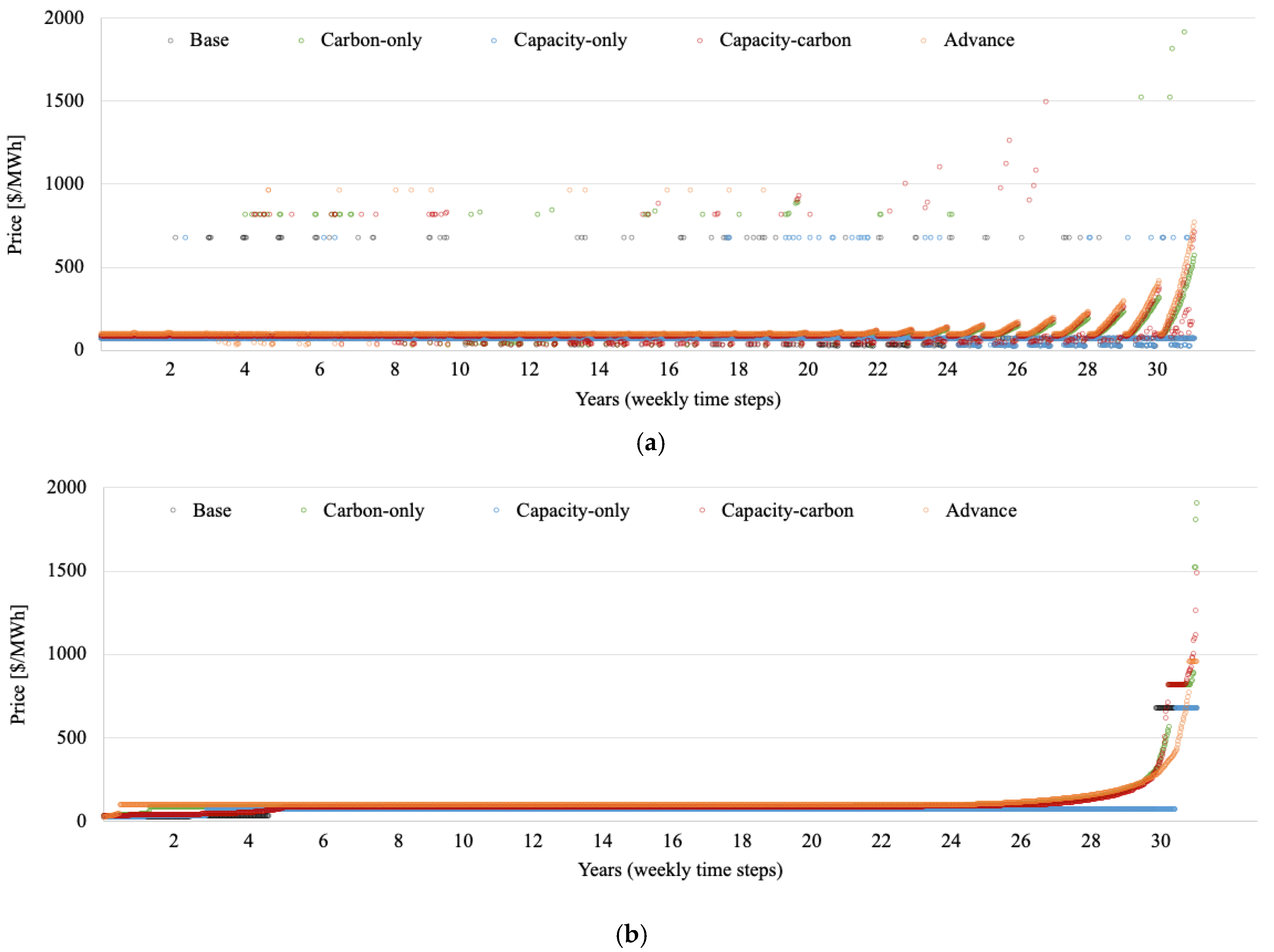
| Base | - | - |
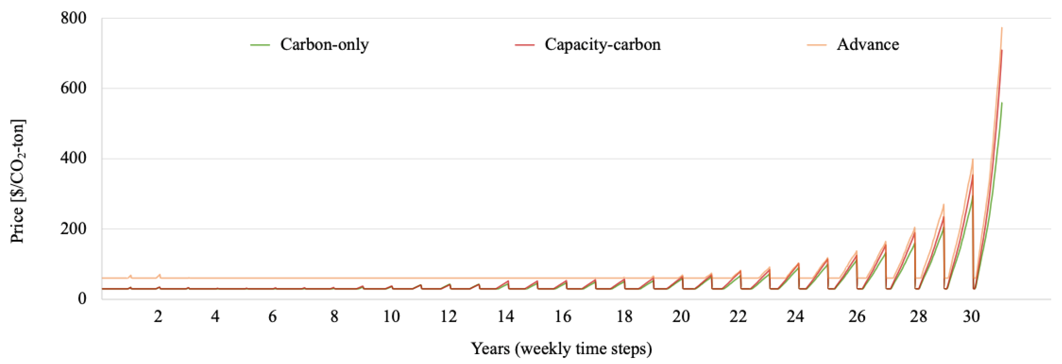
| Carbon-only | USD 30/ton CO2 floor price | - |
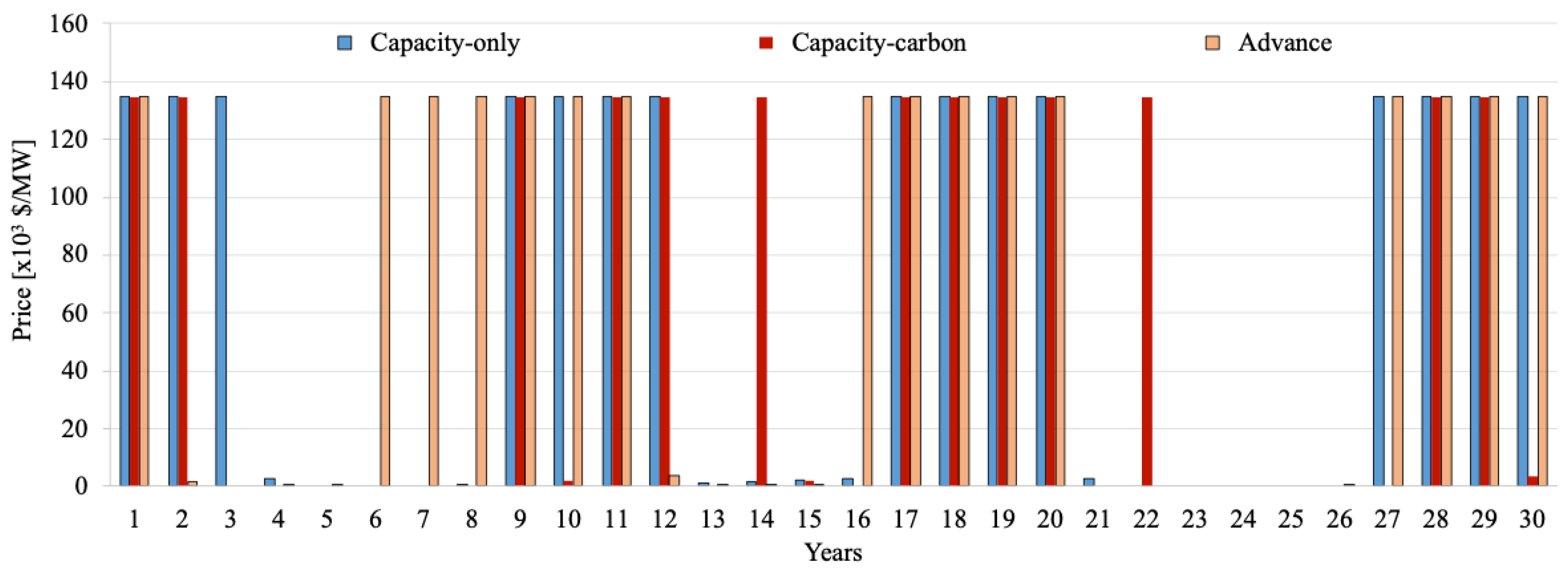
| Capacity-only | - | All fossil fuel power plants |
| Capacity–carbon | USD 30/ton CO2 floor price | All fossil fuel power plants |
| Advance | USD 60/ton CO2 floor price | Flexible power plants |
Publisher’s Note: MDPI stays neutral with regard to jurisdictional claims in published maps and institutional affiliations. |
© 2022 by the authors. Licensee MDPI, Basel, Switzerland. This article is an open access article distributed under the terms and conditions of the Creative Commons Attribution (CC BY) license (https://creativecommons.org/licenses/by/4.0/).
Share and Cite
Luo, Y.; Ahmadi, E.; McLellan, B.C.; Tezuka, T. Will Capacity Mechanisms Conflict with Carbon Pricing? Energies 2022, 15, 9559. https://doi.org/10.3390/en15249559
Luo Y, Ahmadi E, McLellan BC, Tezuka T. Will Capacity Mechanisms Conflict with Carbon Pricing? Energies. 2022; 15(24):9559. https://doi.org/10.3390/en15249559
Chicago/Turabian StyleLuo, Yilun, Esmaeil Ahmadi, Benjamin C. McLellan, and Tetsuo Tezuka. 2022. "Will Capacity Mechanisms Conflict with Carbon Pricing?" Energies 15, no. 24: 9559. https://doi.org/10.3390/en15249559
APA StyleLuo, Y., Ahmadi, E., McLellan, B. C., & Tezuka, T. (2022). Will Capacity Mechanisms Conflict with Carbon Pricing? Energies, 15(24), 9559. https://doi.org/10.3390/en15249559