Article

Online ADMM for Distributed Optimal Power Flow via Lagrangian Duality

1
Chongqing Huizhi Energy Corporation Ltd., State Power Investment Corporation (SPIC), Chongqing 401127, China
2
College of Electronics and Information Engineering, Southwest University, Chongqing 400715, China
3
Key Laboratory of Intelligent Information Processing, Chongqing Three Gorges University, Chongqing 404100, China
4
Chongqing Innovation Center, Beijing Institute of Technology, Chongqing 401120, China
*
Author to whom correspondence should be addressed.
These authors contributed equally to this work.
Current address: Zhongxing Telecommunication Equipment Corporation, Chengdu 610095, China.
Energies 2022, 15(24), 9525; https://doi.org/10.3390/en15249525
Submission received: 28 October 2022 / Revised: 12 December 2022 / Accepted: 13 December 2022 / Published: 15 December 2022

Abstract

:
At present, the power system has the characteristics of mutual independence but interconnection, and the interconnection between the various subsystems brings certain challenges to the distributed computing of the power grid. In addition, a substantial amount of naturally uncertain renewable resources are incorporated into the power system, which will impose volatile dynamics on the grid. In this paper, an alternating direction multiplier method (ADMM) is proposed for the power system with real-time renewables to tackle the online optimal power flow (OPF) problem. Due to the adoption of the Lagrangian duality, the proposed distributed ADMM scheme utilizes consensus ADMM to solve the dual OPF problem, which only discloses boundary coupling via the Lagrangian multiplier and further reduces the amount of information communication. Given the natural uncertainty of distributed energy resources (DER), the algorithm avoids the double-loop implementation or the uncertainty of traditional distributed methods of using the boundary information as equality constraints caused by dynamic DER. It is thus capable of providing a provable performance guarantee and is inherently developed to cope with the dynamic OPF problem with renewables in an online fashion. Taking the IEEE 30-bus system as a test feeder, the simulation results verify the efficiency and robustness of the proposed algorithms in solving both the static and dynamic OPF problems; in addition, the online method can effectively avoid the violent fluctuations of the conventional generator output copying with renewables rapid variation in comparison with the offline algorithms.

1. Introduction

Since the pioneering work on optimal power flow [1] was presented by Carpentier in 1962, his calculation model containing power flow equality and inequality constraints has been an important reference paradigm for realizing the reliable and efficient operation of power systems. This work has attracted attention and obtained a vast amount of research results; please see [2] and the references therein.
OPF aims to determine the economical operating parameters for power systems, minimizing various costs, such as generation cost, line losses, and even consumer disutility. Due to the quadratic relation between the power-related quantities and the voltage phasors [3], the OPF constitutes a nonconvex quadratically constrained quadratic program (QCQP) problem. To deal with this challenge, some (non)linear programming approaches based on gradient descent, Newton-Raphson, and interior-point methods [4] have been put forward to seek solutions satisfying the Karush–Kuhn–Tucker (KKT) condition for local optimality. However, these solutions are often sensitive to initialization. By introducing semidefinite programming (SDP) [2,3,5,6], second-order cone programming (SOCP), and other convex relaxation methods [7] to perform relaxation transformation on the power flow constraints, the nonconvex OPF can be easily resolved. Specifically, the optimal solution of SDP relaxation is a lower bound on the optimal value of the original nonconvex QCQP problem [8].

1.1. Primary Motivations

In the past, solving OPF was usually based on centralized methods [4,6], which assumes that all nodes in the power systems transmit their information to a central operating unit. Actually, the distribution region in a power grid may belong to different owners, and some sensitive information intercepted by malicious attackers might cause financial losses or even security risks. With the wide application of distributed optimization, this situation will be thoroughly changed. As a distributed algorithm, ADMM is naturally suitable for distributed convex optimization, especially for area-based large-scale problems, such as OPF [9,10,11,12,13] and control of reactive power [7,14,15], as well as minimum voltage deviation. Furthermore, ADMM can effectively reduce information disclosure and further preserve local privacy [16].
Currently, the share of variable renewable energy resources, such as wind and solar, is increasing in power systems [17]. Because these DERs are dependent on weather conditions, a variety of technical challenges, such as unpredictability, uncontrollability, and fluctuations in voltage and reactive power [18,19], must be overcome to safely connect them to the grid while maintaining stability and reliability. When integrating DERs into the grid, the power flow distribution will be changed, and the boundary information of each area will also be changed along with it [20]; the original static OPF thus evolves into a dynamic OPF covering multiple continuous time sections [21]. The static OPF finds the optimal solution at a certain time section, regardless of the interrelation among time sections. In the power system with renewables, when the output power of DERs changes rapidly, the generator output in contiguous time sections changes greatly. If continuously adopting the static OPF, the result may cause the generator output to exceed its regulation rate limit between two contiguous time sections, which makes the result infeasible in practice. Therefore, it is imperative to build robustness into power system operation for the dynamic OPF problem against the uncertainties of DERs. Stochastic and robust optimization techniques have been employed to cope with this uncertainty and minimize operational costs [22]. However, these approaches typically require characterizing the uncertainty bounds or the distribution of the DER’s generation output.

1.2. Related Work and Research Gap

Following the above motivation, we survey some related work with the aim of giving a clear understanding of how our algorithm and the results relate to and, in many cases, improve upon it. Our paper is closest to the real-time OPF [23,24,25,26] or online OPF [3,27,28]. For the real-time OPF problem, ref. [23] presented an online gradient projection algorithm, in which the proposed algorithm converges to the set of local optima and an upper bound on the suboptimality gap of any local optimum is also provided as a sufficient condition to guarantee the algorithm converges to a global optimum. Subsequently, ref. [24] developed a real-time algorithm based on quasi-Newton methods, which utilizes second-order information to provide suboptimal power flow solutions. Further extensions of this topic were presented in [25,26] with a look toward the treatment of rapid and economical responses to the changes in the power system operating state by using a deep reinforcement learning method. For the online OPF problem, ref. [3] first sought to study this topic by using an online mirror descent-based algorithm. Besides this, ref. [27] also explored four strategies, including pure numerical, closed form, and numerical hybrids, as well as a Lagrange multiplier method, in which the authors further considered the tradeoff between the time-cost of the solution and guaranteeing a feasible solution. Recently, ref. [28] developed an online algorithm based on the second-order Taylor information in a distributed way by decomposing the sensitivities of the OPF targets among different areas. For more details, please see Table 1.
Despite these efforts, however, there still exist two significant limitations. First, since the OPF problem is nonconvex and may be NP-hard in the worst case, some gradient-based methods, such as [23,24], only guarantee the provision of suboptimal power flow solutions or a local optimum, and guaranteeing the global optimum requires an extra sufficient condition. Although Lavaei and Low [6] have invented a zero duality gap approach used in an SDP optimization for the static OPF problem, it still needs an extra sufficient condition. Second, although the Lagrange multiplier method has been proven in [27] to achieve the fastest solution time for a large-size problem, there are still some underlying problems when applying this method to the real-time or online OPF, such as the decomposition of the large-size OPF into several subproblems, and providing the global optimum for the nonconvex OPF model, as well as guaranteeing zero duality gap without any extra condition, and so on.

1.3. Statement of Contributions

In this paper, inspired by consensus optimization [12,29], we propose an online convex optimization scheme integrating ADMM and Lagrangian duality for resolving the online OPF problem. First, for the static OPF problem, the cost-minimization model referring to [2,11] is built, in which, power flow constraints are constructed via boundary equations comprising the voltage, the phase angle, and the coupling line parameters (admittance, etc.) on the boundary nodes among adjacent areas. To implement the distributed ADMM, we propose a simple area partitioning method based on spectral clustering to provide an optimal partition of the power system. By introducing the Lagrangian duality on the original OPF [30], a global consensus variable is employed as the Lagrangian multiplier for each sub-problem, which is simultaneously copied as a local variable for each sub-area solution [31]. After doing that, the distributed ADMM applied only discloses the boundary coupling information rather than the internal node information so as to avoid determining the coupling equation separately and including the boundary information in the objective function. For the online OPF with renewables, we propose an online convex optimization scheme to tackle the uncertainties of DERs. Specifically, at the beginning of each time slot, the power output of renewable generators must be determined (and fixed) without knowledge of loads; and at the end of the time slot, the loads are revealed so that the power output of conventional generators can be determined under the ramp constraints. The main contributions of the paper are as follows:
  • The Lagrangian duality is utilized to couple the power flow equation and boundary information instead of directly establishing boundary coupling as the ADMM constraint, it can be well adapted to the real-time nature of DESs, such as solar energy, and it can also disclose less boundary information.
  • For the SDP relaxation model of the static OPF, the distributed ADMM is compatibly employed to solve its convex Lagrangian duality problem instead of solving the iterative sub-problem of ADMM under the original nonconvex OPF model.
  • In order to adapt the distributed ADMM to the dynamic OPF with renewables, an online scheme is proposed to cope with the uncertainties of DERs, in which the double-loop implementation is avoided, thus providing a provable performance guarantee.
Notations: The notation “ i ” is reversed for the imaginary unit. Re { A } , Im { A } , and A * represent the real part, imaginary part, and complex conjugation of a given complex scalar A, respectively. The notations A , A H , and rank { A } represent the transpose, Hermitian transpose, and rank of a given matrix A , respectively. For given the notation | x | of absolute-value for a scalar x R , the p -norm ( p 1 ) is defined by x p : = ( | x 1 | p + + | x N | p ) 1 / p for the vector x = [ x 1 , , x N ] R N , which yields the 1 -norm when p = 1 and the Euclidean norm when p = 2 , as well as the -norm when p . Without special statement, · commonly denotes the Euclidean norm. The notation x , y denotes the inner product given by x , y : = x y = i = 1 N x i y i , for x , y R N . Finally, we define the infimum of a set S as the greatest scalar that is less than or equal to all elements of S , abbreviated as inf S ; and denote the argument of the minimum and argument of the maximum for an objective function f by arg min f and arg max f , respectively.
Table 1. Comparisons of the proposed algorithm with the existing distributed online algorithms.
LiteratureTopicAC/DCRenewablesApproach
[30]Dynamic OPFDCN/ADistributed dual consensus ADMM
[23]Real-time OPFACN/AOnline gradient projection
[24]Real-time OPFACN/AQuasi-Newton methods
[25,26]Real-time OPFACN/ADeep reinforcement learning
[27]Online OPFDCN/ALagrange multiplier method
[3]Online OPFACWind turbineOnline mirror descent
[28]Online OPFACPhotovoltaicSecond-order Taylor-based gradient
ours.Online OPFACPhotovoltaicOnline ADMM Lagrangian duality

2. Model and Formulation

2.1. Optimal Power Flow Formulation

Considering a power network with the set of buses N : = { 1 , 2 , , N } , the set of flow lines E N × N between the buses. Let Ω n : = { n | ( n , n ) E } be the set of buses connected to bus n, where n N is the index. Denote the complex voltage amplitude and the injected current at bus n by V n and I n , respectively. Each line ( n , n ) E of the network is modeled as a passive device with an admittance y n n , thus the network can be modeled as a general admittance matrix Y C N × N whose ( n , n ) -entry is formed as
Y n n = y n 0 + n Ω n y n n , if n = n y n n , if n n , ( n , n ) E 0 , otherwise
where y n 0 is the admittance-to-ground of bus n, which is normally not considered for the OPF modeling. Then, Kirchhoff’s and Ohm’s laws yield
I n = n Ω n ( V n V n ) y n n ,
which means the complex power injected to bus n can be given by
S n : = P n + i Q n = V n I n * = V n n Ω n ( V n V n ) * y n n * ,
where P n and Q n represent the active power and reactive power injected to bus n, respectively.
We denote the set of buses with conventional generators and renewable generators by N G N and N R N , respectively. Let P n G and Q n G be the active power output and reactive power output of the conventional generator at bus n N G , respectively. Similarly, let P n R and Q n R be the active power output and reactive power output of renewable power, such as photovoltaic energy, wind power, and geothermal energy, generated by bus n N R , respectively. Finally, let P n D and Q n D be the active load and reactive load at bus n N , respectively. Then, the power balance condition of each bus n N can be formed as
P n = P n G + P n R P n D ,
Q n = Q n G + Q n R Q n D .
It should be noted here that P n G = Q n G = 0 , if n N while n N G , and all else follows.
Ref. [2] has formed four types of line capacity constraints, which are can achieve various goals in practice, such as avoiding line overheating and guaranteeing the stability of the network. To simplify the problem, researchers generally select one of them as the line capacity constraint [3]:
V n V n Δ V n n max
where Δ V n n max represents the maximum voltage difference over line ( n , n ) , this limitation is equivalent to the line current magnitude constraint, since each line has been modeled as a simple admittance and it follows from (2) that V n V n is proportional to the line current.
Now, we turn to formulating the OPF problem. We consider the minimization of system operating cost as the objective function, and the power flow balance, line capacity limitation, generator capacity limitation, and voltage amplitude limitation as constraints. Specifically, the mathematical formulation of OPF is given as
minimize V , P G , Q G n N G f n P n G
subject to P n G + P n R P n D = n Ω n Re { V n ( V n * V n * ) y n n * }
Q n G + Q n R Q n D = n Ω n Im { V n ( V n * V n * ) y n n * }
P n min P n G P n max
Q n min Q n G Q n max
V n min V n V n max
V n V n Δ V n n max
where V , P G , P R , P D , Q G , Q R , and Q D are the vector forms of V n , P n G , P n R P n D , Q n G , Q n R , and Q n D for n N , respectively. Equations (6b) and (6c) are the power balance conditions accounting for the conservation of power at bus n, yielded by (3), (4a), and (4b). Equations (6d), (6e), and (6f) restrict the active power, reactive power, and voltage magnitude at bus n, respectively, for given limits P n min , Q n min , V n min , P n max , Q n max , and V n max . Objective (6a) can capture various costs, such as generation cost, line losses, conservation voltage reduction, etc. Generally, the generation cost is modeled by a quadratic function form as:
f n P n G : = α n P n G 2 + β n P n G + γ n
where α n 0 , β n , and γ n represent the cost parameters of the generator at bus n N G . In a nutshell, OPF minimizes the total cost n N f n over the unknown parameters V , P G , and Q G , for given the known vector P R , P D , Q R , and Q D , subject to some constraints.

2.2. Convex Relaxation Approach to OPF

It should be noted here that objective (6a) of OPF is convex while the constraints are nonconvex due to the nonlinear terms V n and V n V n * . Since solving nonconvex optimization is pretty hard, ref. [6] suggested a convex relaxation of the OPF problem by defining W : = V V H , then OPF constraints containing the quadratic item V n V n * can be expressed as a linear function of W . In order to ensure that the nonconvex OPF is transformed into an equivalent form, it requires that W is Hermitian and positive semidefinite with rank { W } = 1 . Hence, the only source of nonconvexity in the equivalent OPF problem comes from the ‘rank-1’ constraint. Motivated by the technique of convex relaxation, after dropping the rank constraint rank { W } = 1 , the nonconvex OPF problem has been formulated as a rank-relaxed semidefinite programming problem:
minimize W 0 , P G , Q G n N G α n P n G 2 + β n P n G + γ n
subject to P n G + P n R P n D = n Ω n Re { ( W n n W n n ) y n n * }
Q n G + Q n R Q n D = n Ω n Im { ( W n n W n n ) y n n * }
P n min P n G P n max
Q n min Q n G Q n max
V n min 2 W n n V n max 2
W n n + W n n W n n W n n Δ V n n max 2
which can be solved using the interior-point method. Although the convex relaxation approach has nearly changed the original problem, if the original problem possesses a certain nice structure and the relaxation is also carefully performed, then the relaxation gaps are almost absent, i.e., solutions to the relax problem would be optimal for the original nonconvex problem as well.

2.3. Area Partitioning Based on Spectral Clustering

The scale of actual power grids is usually large, so the overall OPF problem of the whole power grid is very complex and is hard to solve directly. Fortunately, the voltage issues are usually regional [11]. Therefore, we can try to partition the whole power grid into several sub-regions such that the OPF problem can be decomposed into several sub-problems, thus decreasing the difficulty of solving the overall OPF problem.
In this subsection, we propose a simple partitioning method based on spectral clustering [32] for providing an optimal partition of the power system. Spectral clustering is a graph partitioning method that takes into account the affinity between any two nodes in the target graph, which in our considered problem, corresponds to the computational coupling between any two buses. Specifically, such coupling relation is reflected in the admittance matrix, but the admittance matrix cannot be regarded as the Laplacian matrix directly due to the complex admittance. Hence, modular operation is essential for constructing the Laplacian matrix. In the proposed method, the k-means algorithm [33] helps to implement clustering so that the inaccuracy in clustering nonconvex regions can be avoided. First, we fix the number of sub-regions by K, then find the optimal way to partition the system into this number of fixed sub-regions. The whole procedure is given by:
(1).
Construct the Laplacian matrix L . Denote the nondiagonal entry of L by the negative modulus of its corresponding complex admittance and the diagonal entry of L by the sum of the complex admittance modulus, i.e.,
L n n = n Ω n | y n n | , if n = n | y n n | , if n n , ( n , n ) E 0 , otherwise .
(2).
Find the K largest eigenvalues of L and form the matrix U R N × K by stacking the corresponding eigenvectors u 1 , , u K as columns.
(3).
Let v n R K be the vector corresponding to the n-th row of U , n = 1 , , N . Cluster the points { v n } n = 1 N with the k-means algorithm into clusters C 1 , , C K .
(4).
Assign bus n to cluster C k if the n-th row of U was assigned to cluster C k .

3. Distributed ADMM for Static OPF

3.1. Lagrangian Duality Based on Partition

As described above, the power system can be divided into multiple sub-regions, and a local OPF problem can be formulated for each sub-region. Assuming that there are a total of K sub-regions. Denote the set of buses in the k-th sub-region by R k satisfying R k R = if k , and the number of buses in the k-th sub-region by | R k | . For region k, define the variable x k : = { ( W n , P n , Q n ) n R k } , which covers the variable x n on each node n, and represents the original variable of each region, the OPF problem can be re-formulated by a local sum form based on variable x k as:
minimize x k X k k = 1 K F k x k : = k = 1 K n R k f n x n
subject to g k x k = 0
h k x k 0
where X k represents the local feasibility constraint set defined by X k : = x k ( 8 b ) ( 8 g ) , the power flow constraint g k x k is expressed as equation constraints in the original OPF problem, i.e., (8b) and (8c), and the line transmission capacity limit h k x k is expressed as inequality constraints in the original OPF problem, i.e., (8d)–(8g).
After the OPF model of each sub-region is given, a common practice is to duplicate the voltage phase angle or the transmitted power at boundary buses of each region [11]. This approach will remove the tie lines between connected regions, which makes the OPF problem more easily solved in a decentralized manner. However, it also has one major disadvantage; it needs to determine more coupling conditions. Especially if renewable energy integrates into the power grid, which will lead to power flow fluctuations, this approach may face some difficulties in solving the dynamical OPF problem under multiple time sections.
In order to avoid the determination of the coupling equations, we define the Lagrangian D k ( x k ; λ , μ ) associated with the original problem (9), which takes the constraints in (9) into account by augmenting the objective function with a sum of the constraint functions. Mathematically, it is given by:
D k ( x k ; λ , μ ) : = n R k f n x k + λ n R k g n x k + μ n R k h n x k
where the global variables λ 0 and μ are the Lagrange multipliers that are introduced for the equality constraint and the inequality constraint, respectively. Now we define the Lagrangian duality Function (LDF) as the minimum value of the Lagrangian over x k :
LDF ( λ , μ ) = inf x k X k k = 1 K D k ( x k ; λ , μ ) .
which aims at solving the Lagrangian (10) with respect to x k by maximizing LDF ( λ , μ ) with respect to λ and μ rather than x k . Because the original problem (9) is convex, according to Slater constraint qualification [34], the duality gap between (9) and its dual problem is zero. Therefore, we can obtain the solutions to problem (9) by solving its dual problem max LDF ( λ , μ ) . The advantage of this is that the constraints in (8b), (8c), and (8g) (or equivalently (9b) and (9c)) are coupled, and it is difficult to decompose these constraints into several independent subproblems, but the dual function can be easily decomposed into several independent maximizations based on region partitioning.

3.2. Distributed ADMM for Lagrangian Duality

In order to distributedly solve the Lagrangian duality, this paper adopts ADMM [16], which can divide a complicated problem into multiple simple sub-problems, and each sub-problem can be solved independently and locally by the data provider. Thus it is suitable for dealing with the Lagrangian duality based on area partitioning. However, the local Lagrangian (10) contains two global variables λ and μ that are not desired. To this end, we introduce a local variable z k for the k-th region to copy the global variable y : = [ λ ; μ ] as an equation constraint, then the Lagrangian duality problem can be transformed into an equivalent distributed minimization problem with local variable z k : = [ λ z , k ; μ z , k ] and consensus variable y :
minimize x k X k k = 1 K D k ( x k ; z k ) subject to y z k = 0
which has been suitable for ADMM to solve distributedly. We denote the Lagrangian multiplier by σ : = [ σ 1 , , σ K ] with σ k : = [ λ σ , k ; μ σ , k ] and the penalty factor by ρ > 0 , one can get the augmented Lagrangian function of problem (12):
L ( y , z ; σ ) : = k = 1 K D k ( x k ; z k ) + σ k , y z k + ρ 2 y z k 2 .
where z : = [ z 1 , , z K ] . For a given interval ρ [ 0 , ρ ¯ ] , one can evolve the penalty factor ρ by a similar Logarithmic barrier indicator function, i.e., I ( ρ ) = ( 1 / c ) log ( ρ ρ ¯ ) with a constant c = 1 / 2 , 1 or 2. Note that in the method of multipliers, updating the dual variable uses a step-size equal to ρ . ADMM consists of the following three iterations with index τ :
y τ + 1 : = arg min y L ( y , z τ ; σ τ )
z k τ + 1 : = arg min z k L ( y τ + 1 , z ; σ τ )
σ k τ + 1 : = σ k τ + ρ y τ + 1 z k τ + 1 .
In order to resolve the problem (13), ADMM needs to be rewritten in a more intuitive form.
(1). The update of consensus variable y :
Since the constant term cannot change the optimization solution of y , removing the constant term yields a precise form:
y τ + 1 : = arg min y k = 1 K σ k τ y + ρ 2 y z k τ 2 .
It is easy to see that (14) is a convex quadratic function of y , which can be solved by taking the derivative to 0:
y τ + 1 = 1 K k = 1 K z k τ 1 ρ σ k τ .
(2). The update of local variable z k :
Similarly, removing the constant term yields a precise form:
z k τ + 1 : = arg min z k D k x k ; z k σ k τ , z k + ρ 2 y τ + 1 z k 2 .
Substituting (10) into (16) yields
z k τ + 1 = arg min z k arg min x k X k n R k f n x k + λ z , k n R k g n x k + μ z , k n R k h n x k σ k τ , z k + ρ 2 y τ + 1 z k 2 = arg max z k arg min x k X k n R k f n x k + n R k g n x k ; n R k h n x k + σ k τ , z k ρ 2 y τ + 1 z k 2 }
where we use the denotation z k = [ λ z , k ; μ z , k ] . Since the duality gap between (9) and its dual problem is zero, there is a saddle point S ( x ¯ k , z ¯ k ) [31] such that
arg max z k arg min x k X k S ( x k , z k ) = S ( x ¯ k , z ¯ k ) = arg min x k X k arg max z k S ( x k , z k ) .
Hence, (17) is equivalent to
x k τ + 1 = arg min x k X k arg max z k n R k f n x k + n R k g n x k ; n R k h n x k + σ k τ , z k ρ 2 y τ + 1 z k 2 } .
For any fixed x k , the maximum on the right-hand side of (18) is uniquely attained by the following update step:
z k τ + 1 = λ z , k τ + 1 μ z , k τ + 1 = λ y τ + 1 + 1 ρ n R k g n x k + λ σ , k τ max 0 , μ y τ + 1 + 1 ρ n R k h n x k + μ σ , k τ
where we note that the inequality constraint h n ( x k ) 0 is equivalent to max { 0 , h n ( x k ) } . For the determined z k τ + 1 , substituting (19) into (18), one has
x k τ + 1 = arg min x k X k n R k f n x k + ρ z k τ + 1 y τ + 1 , z k τ + 1 ρ 2 y τ + 1 z k τ + 1 2 = arg min x k X k n R k f n x k ρ 2 y τ + 1 2 + ρ 2 z k τ + 1 2
where the term ρ 2 y τ + 1 2 in (20) is seen as a constant for x k τ + 1 and cannot change the optimal solution. Hence, x k τ + 1 is a solution to the following minimization problem:
x k τ + 1 = arg min x k X k n R k f n x k + ρ 2 λ y τ + 1 + 1 ρ n R k g n x k + λ σ , k τ max 0 , μ y τ + 1 + 1 ρ n R k h n x k + μ σ , k τ 2 .
(3). The update of Lagrange multipliers σ k :
The Lagrange multipliers are locally stored and updated according to (13c) for each area k { 1 , , K } , where all variables involved in this step have been calculated and communicated in the update of y and z k .
After analyzing the intrinsic update procedure of ADMM, it is easy to see that only the update of z k involves the exchange of information between regions, and once the updated information is obtained from the adjacent regions, it can also be calculated locally. The update of y needs to separately solve a quadratic programming problem while updating the Lagrangian multiplier σ k is the simplest to carry out. Therefore, ADMM can be implemented in a completely distributed manner, requiring only local information exchange without centralized coordination. The distributed algorithm for the OPF problem eliminates the steps of separately determining the boundary coupling equation and coupling information and utilizes the power flow equation to construct the Lagrangian, which reduces the disclosure of boundary information to a certain extent.
The convergence of ADMM is judged by the original residual r τ and the dual residual s τ defined as
r τ = y τ z 1 τ ; ; y τ z k τ ; ; y τ z K τ , s τ = ρ z 1 τ z 1 τ 1 ; ; z k τ z k τ 1 ; ; z K τ z K τ 1 .
When r τ 2 ε 1 and s τ 2 ε 2 for given error bounds ε 1 and ε 2 , the iteration stops and the optimal solutions are obtained.

4. Distributed ADMM for Online OPF

The previous sections investigate the OPF problem in a single gap and its solution; however, the whole model and solving procedure are based on the assumption that the power output of renewable sources remains unchanged such that an OPF solution in a single gap can be obtained. In the actual electric grid, the renewable power sources, especially the photovoltaic and wind turbine, are usually time-varying and fluctuate due to their uncertainty and unpredictability, which deduces a dynamic OPF problem. If we solve the dynamic OPF with a long time scale, the previous approach will lead to a double-loop implementation.
In order to avoid the double-loop implementation, we present an online ADMM to address the dynamic OPF problem with the fluctuated renewable energy and real-time loads. This is a completely distributed algorithm that makes the optimal decision in each time slot and only needs to know the instantaneous system state.

4.1. Online Convex Optimization

Recent studies showed that many online learning algorithms are designed based on online convex optimization tools, whose decision set is a convex set X R N in N-dimensional Euclidean space, and costs are a series of bounded convex functions defined on the convex set X . Online convex optimization can be regarded as a repeated game. At time t, the player chooses an action x t X , then the adversary reveals a convex loss function c t : X R N . The player’s goal is to minimize the regret R c ( T ) on the number of time slots T, which is defined as:
R c ( T ) : = t = 1 T c t x t min x X t = 1 T c t ( x ) .
Under the appropriate hypotheses, well-constructed online learning algorithms can achieve a regret bound that grows sublinearly in T, i.e., lim T R c ( T ) / T = 0 .

4.2. Online OPF Formulation

The dynamic OPF problem based on online convex optimization can be stated as follows. At each time slot t { 1 , 2 , , T } , on the basis of the realizations observed so far for the renewable sources { P n R , τ , Q n R , τ } τ = 1 t and the loads { P n D , τ , Q n D , τ } τ = 1 t , find the OPF { P n R , t + 1 , Q n R , t + 1 } in the next time slot, so as to minimize the regret. Specifically, the loss function at time slot t can be formed as
c t x t : = k = 1 K D k t ( x k t ; λ t , μ t )
where D k t ( x k t ; λ t , μ t ) is an online version (at time slot t) of the Lagrangian D k ( x k ; λ , μ ) , defined in (10), associated with the OPF problem in a single gap. Since the dual function (11) is the pointwise infimum of a family of affine functions of ( λ , μ ) , it is concave, even when the original problem (9) is not convex [34]. Hence, the loss function c t ( x t ) is convex, and then the Lagrangian duality of the dynamic OPF problem can be solved by an online learning algorithm based on the online convex optimization technique.

4.3. ADMM for Online OPF

Considering the advantage of the ADMM framework and avoid a double-loop implementation, we adopt the online ADMM approach [35] to solve the following optimization problem
minimize x k X k t = 1 T k = 1 K D k t ( x k ; z k ) subject to y z k = 0
in an online fashion. The augmented Lagrangian is given by
L t ( y , z ; σ ) : = k = 1 K D k t ( x k ; z k ) + σ k , y z k + ρ 2 y z k 2 .
From which we can obtain the update steps of the online ADMM approach:
y t + 1 : = arg min y L t ( y , z t ; σ t ) = 1 K k = 1 K z k t 1 ρ σ k t
z k t + 1 : = arg min z k L t ( y t + 1 , z ; σ t ) = λ y t + 1 + 1 ρ n R k g n x k + λ σ , k t max 0 , μ y t + 1 + 1 ρ n R k h n x k + μ σ , k t
σ k t + 1 : = σ k t + ρ y t + 1 z k t + 1 .
At each time slot t, the online ADMM updates multiplier vectors y t and z k t to solve variable x k t + 1 from the following minimization problem in an online fashion:
minimize x k X k n R k f n x k + ρ 2 λ y t + 1 + 1 ρ n R k g n x k + λ σ , k t max 0 , μ y t + 1 + 1 ρ n R k h n x k + μ σ , k t 2 .
The above procedure can be summarized in Algorithm 1. The iteration complexity of the online ADMM has been extensively studied in the literature (see [35] and the references therein). It can be shown that the iterate { x t } achieves a sublinear regret bound, i.e., R c ( T ) = O ( T ) , under some mild conditions on the problem.
Algorithm 1 Online ADMM for OPF.
Initialize: z k 0 , σ k 0 , ρ > 0 , and T N
1:
for each time slot t = 1 , , T do
2:
 Calculate constraints g n ( x k t ) & h n ( x k t ) according to online data P n D , t , Q n D , t , P n R , t , Q n R , t
3:
 Obtain y t + 1 according to (25a)
4:
for each sub-region k = 1 , , K do
5:
    Calculate x k t via solving (26)
6:
    Update z k t + 1 using (25b)
7:
    Update σ k t + 1 using (25c)
8:
 end for
9:
end for
It is worth noting that, at each time slot t, the online data stream will be fed to the online ADMM based on a single-loop iterative implementation, which strives for faster convergence. Recently, some variants of ADMM were studied that exhibit faster convergence rates while requiring only a little change in the computational effort of each iteration [36]. Here we adopt a practical, efficient method, the Peaceman–Rachford Splitting Method (PRSM) [37], to accelerate ADMM. Specifically, by adding an intermediate multiplier and introducing an underdetermined relaxation factor ξ ( 0 , 1 ) , the PRSM-ADMM can ensure strict convergence, and its convergence rate is also faster than ADMM. Mathematically, the update rule of the intermediate multiplier in PRSM-ADMM is given by
σ k t + 0.5 : = σ k t + ξ ρ y t + 1 z k t .
Then, we update z k t according to the new rule
z k t + 1 : = λ y t + 1 + 1 ρ n R k g n x k + λ σ , k t + 0.5 max 0 , μ y t + 1 + 1 ρ n R k h n x k + μ σ , k t + 0.5 .
The final update rule of the multiplier in PRSM-ADMM is
σ k t + 1 : = σ k t + 0.5 + ξ ρ y t + 1 z k t + 1 .
The whole procedure can be summarized in Algorithm 2.
Algorithm 2 Online PRSM-ADMM for OPF.
Initialize: z k 0 , σ k 0 , ρ > 0 , ξ ( 0 , 1 ) and T N
  1:
for each time slot t = 1 , , T do
  2:
 Calculate constraints g n ( x k t ) & h n ( x k t ) according to online data P n D , t , Q n D , t , P n R , t , Q n R , t
  3:
 Obtain y t + 1 according to (25a)
  4:
for each sub-region k = 1 , , K do
  5:
    Calculate x k t via solving (26)
  6:
    Update σ k t + 0.5 using (27)
  7:
    Update z k t + 1 using (28)
  8:
    Update σ k t + 1 using (29)
  9:
end for
10:
end for

5. Numerical Tests

In this section, we illustrate the use of the distributed ADMM on static and dynamic case studies to find the optimal power flow under equation and inequality constraints.

5.1. Simulation Setup and Area Partitioning

The distributed ADMM algorithms are tested on the IEEE 30-bus system, which contains 6 motors and 21 loads. The generator and load adopt IEEE 30-bus standard data, but the load adopts a 24-h spinning reserve, and adding random noise corresponds to the solar data. The photovoltaic solar panels used in this article as generators produce electricity in DC, which needs to transform into AC via an inverter for feeding the electric grid. In this experimental environment, the grid-tied system with the photovoltaic does not need battery storage because the grid acts as a power reserve. If the grid goes down, the inverter automatically shuts off and will not feed solar-generated electricity back into the grid. Therefore, the photovoltaic can be safely incorporated on the designated node to perform distributed power flow calculation [38], whose access points should be relatively concentrated and located as close to the reference node as possible so as to reduce the harmonics caused by grid connection and the impact on the grid. For a typical photovoltaic module [39], the max power is 300W; the voltage and current at maximum power points are 50.6 V and 5.9 A, respectively, and the open-circuit voltage and short-circuit current are 63.2 V and 6.5 A, respectively. The solar data were extracted from an open-source dataset (https://www.elia.be/, accessed on 20 October 2022). Fifteen-minute-sampled solar generation data were collected on 18 July 2020, from 00:00 to 24:00. Considering the power generation capacity and the standard unit value, the data at each time slot were standardized. For a typical DC/AC inverter [39], the input and output voltages are 354 and 230 V, respectively; the power rating is 10 kW; and the amplitude and frequency modulation index are 0.92 and 100, respectively.
Section 2.3 introduced the area partitioning approach based on spectral clustering. The partitioning is chosen such that each load bus is assigned to the same area in line impedance as its nearest generator bus. After defining the Lagrangian matrix based on the complex admittance of the IEEE 30-bus system, we simply calculate the K-largest eigenvalues (here K = 2 , 3 ) and cluster all of the buses into K regions. Among them, the Optimal (region) Partition by using the spectral clustering-based method proposed in this paper, is represented by O P ( K ) , and the other partitions based on the electrical distance between buses [40] or the simpler index clustering are represented by N P ( K ) . Specifically, in [40], the regions are partitioned in the way that each load is assigned to the same region as its closest generator in terms of line impedance. After that, we obtain the coupling parameter, 0.6117 and 0.7532 determine the optimal partitioning plan { ( 1 8 , 28 ) ; ( 9 27 , 29 30 ) } and { ( 1 8 , 25 30 ) ; ( 9 20 ) ; ( 21 24 ) } as the O P ( 2 ) and O P ( 3 ) in Figure 1a, and the specific information are shown in Table 2.

5.2. Static OPF Simulation

In this simulation part, the maximum number of iterations M = 2000 and the original residual and dual residual iteration stop criteria are set to ε 1 = ε 2 = 1 × 10 4 .
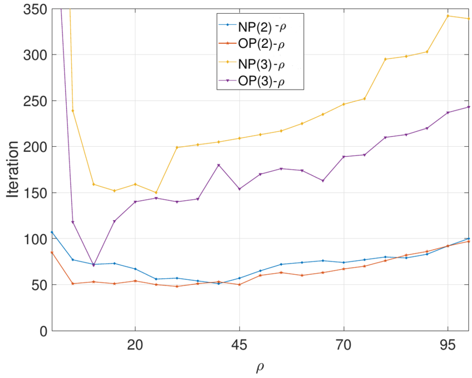
First, we discuss the influence of the dual update step size ρ in (13) on the number of iterations in different area partitioning cases. Figure 2 shows that the optimal dual update step size corresponding to three partition cases may be different. In that, we traverse ρ [ 1 , 100 ] N to roughly determine the optimal value ρ * = 15 for the same residual accuracy, which will guarantee that the distributed ADMM can converge at the fastest speed. The figure also shows that O P ( 3 ) is more sensitive to the value of ρ , which means the selection of ρ will profoundly affect the convergence performance in this case.
The number of border branches and the number of global variables correspond to the Lagrangian multiplier variable y = ( λ ; μ ) in (10), as well as the number of iterations for the given residual accuracy. Obviously, the more variables are involved, the more iterations are needed to achieve the same residual accuracy.
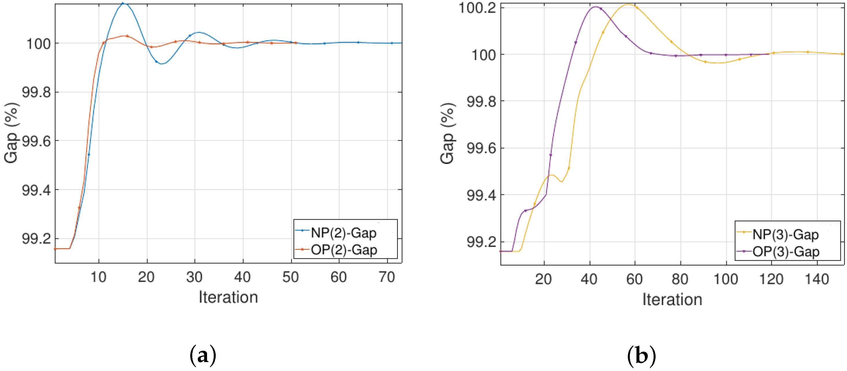
When the dual step size ρ = 15 , the convergence results of the distributed ADMM are discussed. Figure 3a,b show the relative error (expressed as a percentage) of the target value obtained by ADMM at each iteration over a single slot (assuming that the dynamic data of formula (4a) and (4b) are fixed) with respect to the target value obtained by the centralized method (the exact value), expressed as the gap in the target value. A set of comparisons is made between the optimal partition and the conventional partition with the same number of regions K. Since ADMM gradually converges to the optimal value during each iteration, the gap between the target value obtained by the centralized method will be narrowed in the case of convergence. As shown in Figure 3a,b, all four methods have considerable convergence effects, but ADMM with O P ( K ) converges faster than that with N P ( K ) and achieves a shorter oscillation period. It is worth noting here that there is a clear rise in Figure 3a,b, which is caused by changes in the penalty parameter. At the beginning of the iteration, the subproblems tend to find better local optima with little regard for connections to other subproblems, which leads to a gap oscillation.
The comparison of public information between the method in [40] and ours is shown in Table 3, which gives the differences in iteration number and running time for the same accuracy as well as other parameters, etc. Obviously, our method is significantly superior to [40] in convergence time. It is worth noting that N P ( 2 ) may be superior to O P ( 2 ) in the gap factor, but O P ( 2 ) has better accuracy performance for the same iteration number, which has also been verified by Figure 4. It is clear that the amount of public information in our method is significantly less than [40]. Moreover, our method only needs the number of boundary branches between adjacent subsystems to calculate the amount of public information, while [40] additionally needs to consider the partition strategy on the basis of knowing the number of boundary branches.
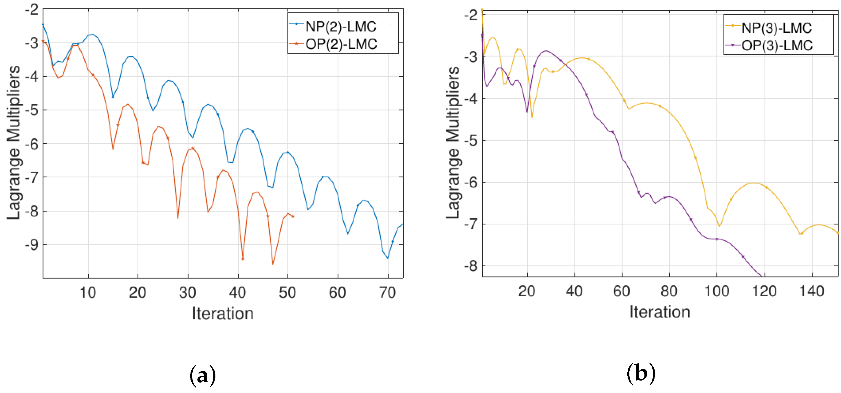
Note that the convergence of the Lagrangian multiplier is also an important criterion for judging whether the algorithm is optimal. Let LMC = log σ τ + 1 σ τ , where log · represents the logarithm of the infinite norm. Figure 4 depicts the iteration of multiplier σ and shows good convergence performance of the algorithm in three cases, especially for O P ( 2 ) and O P ( 3 ) , which also verifies the conclusion suggested in Figure 3. In order to solve the single-slot OPF problem, the proposed SDP relaxation scheme incorporated into the distributed ADMM can achieve better convergence and robustness, as shown in Figure 4.
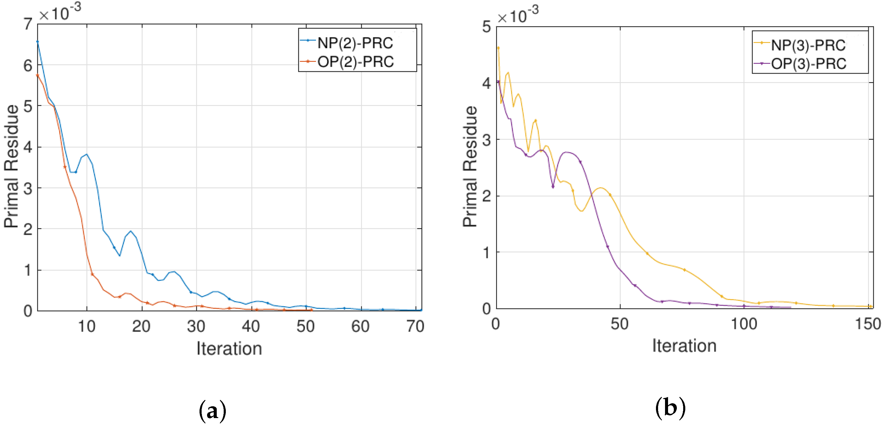
In Figure 5, we evaluate the convergence of the primal residuals of ADMM. We use PRC to record the convergence process of the primal residual before which the residual termination condition is defined. Like LMC , O P ( K ) has a better convergence speed than N P ( K ) and reaches the termination condition faster with the same number of partitions.
This section focuses on the performance of the proposed distributed ADMM algorithm on SDP-OPF. After the test of the indicators, the effectiveness of the algorithm can be seen. In the four partitioning schemes, the algorithms have high accuracy and fast convergence performance. The spectral clustering method further shows its effectiveness in improving the system performance under the same number of regions. However, the modified algorithm has good adaptability to dynamic online problems because it bypasses the boundary coupling equation in essence. To better simulate the time-varying DER injected into the power grid, we introduce an online OPF model, which will be further elaborated upon in the next subsection.

5.3. Online OPF Simulation

This subsection tests the performance of the online ADMM, which will monitor the real-time data of solar-power generation and make the best decision due to its intermittency and uncontrollability. We still adopt the IEEE 30-bus system to be injected photovoltaic generators, as shown in Figure 1b, where the set of solar power buses is 2 , 3 , 14 , 17 , 24 , the set of conventional generator buses 1 , 2 , 5 , 8 , 11 , 13 , and buses 7 , 12 , 19 , 21 , 30 will be used later. We still use O P ( 2 ) as the area partitioning scheme due to its good performance in the static scene, which is not shown in Figure 1b for considering a more clean picture.
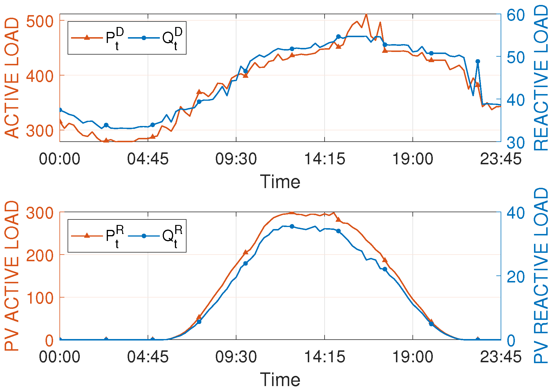
Figure 6 shows the active/reactive load data P n , t D and Q n , t D , as well as the active/reactive solar power output data P n , t R and Q n , t R , which can be found on the same website (https://www.elia.be/, accessed on 10 October 2022). Solar-power output is affected by weather and seasonal variations. The angle of the sun to the solar panel changes with the time of day and seasonal variations. Cloudy and rainy days also contribute to less effectiveness of sunlight collection. The sampling period is one day, and the sampling length is 24 h. Generally, the increase in load will naturally affect the output of generators, and various DESs may be our best way to offset the instantaneous power difference.

5.3.1. Performance Comparison

This subsection investigated the performance comparison of the proposed online algorithm with the closest literature [30]. In [30], the authors solved the static DC-OPF problem by ADMM and Lagrangian duality, while our paper addressed the static and dynamic AC-OPF problem. In order to perform the comparison, we develop a quasi-static distributed OPF problem to reduce the difference, in which we need to rewrite the cost function as the minimum economic operation index; then convex relaxation can be carried out. The resulting optimization problem can continue to perform the comparison with our algorithm in distributed OPF calculation.
For coming into use of the offline algorithm [30], at the end of time slot t 1 , we assume that the solar power generation of time slot t is the same as that of time slot t 1 (persistence prediction), the active power output is determined by solving a distributed OPF problem. Specifically, it is to solve the following problems:
minimize W 0 , P G , t , Q G , t n N G α n P n G , t 2 + β n P n G , t + γ n
subject to P n G , t + P n R , t 1 P n D , t 1 = n Ω n Re { ( W n n W n n ) y n n * }
Q n G , t + Q n R , t 1 Q n D , t 1 = n Ω n Im { ( W n n W n n ) y n n * }
P n min P n G , t P n max
Q n min Q n G , t Q n max
V n min 2 W n n V n max 2
W n n + W n n W n n W n n Δ V n n max 2
In time slot t, after the actual solar power generation is realized, OPF is solved again. The total cost of the static algorithm is also n N G α n ( P n G , t ) 2 + β n ( P n G , t ) + γ n . Note that this offline scheme needs to solve the distributed OPF problem twice in each time slot, while the online scheme proposed in our paper only solves the OPF problem once in each time slot.
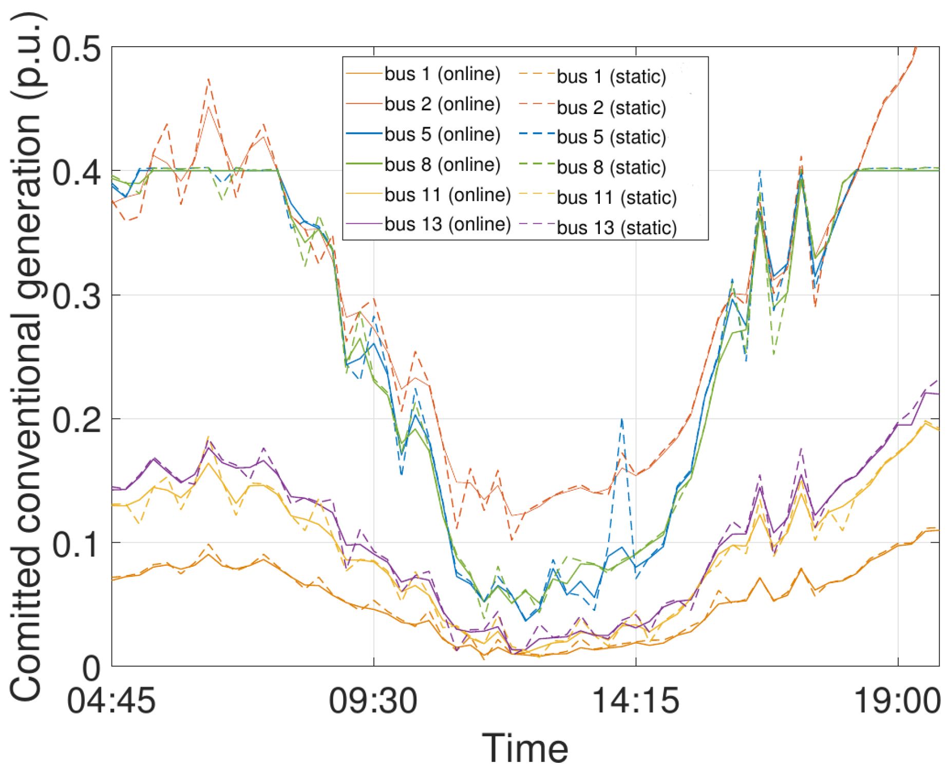
Figure 7 shows the evolution of total cost between the offline [30] and online algorithms for solving the distributed OPF, in which we still use solar power generation in Figure 6. As a whole, it can be seen that the overall online scheme is smoother than the offline scheme. In particular, when the solar power generation capacity suddenly drops or increases, the cost of the online scheme is much lower than the offline scheme. This is because the offline scheme fully trusts the prediction of renewable energy power generation and significantly reduces or increases the conventional power generation that has been invested, while the online scheme in our paper considers the impact of time-scale, which has a better performance in long-range dependence. Therefore, the online scheme can avoid the power output of conventional generators instantaneously surging when the power generation of renewables drops sharply. This conclusion has been confirmed in Figure 8, which describes the conventional power generation submitted by the offline [30] and online schemes in each time slot. It is known from Figure 6 that solar injection basically affects the power grid from the period 04:45–19:30; thus Figure 8 only intercepts the power generation in this period.

5.3.2. Online Performance Analysis

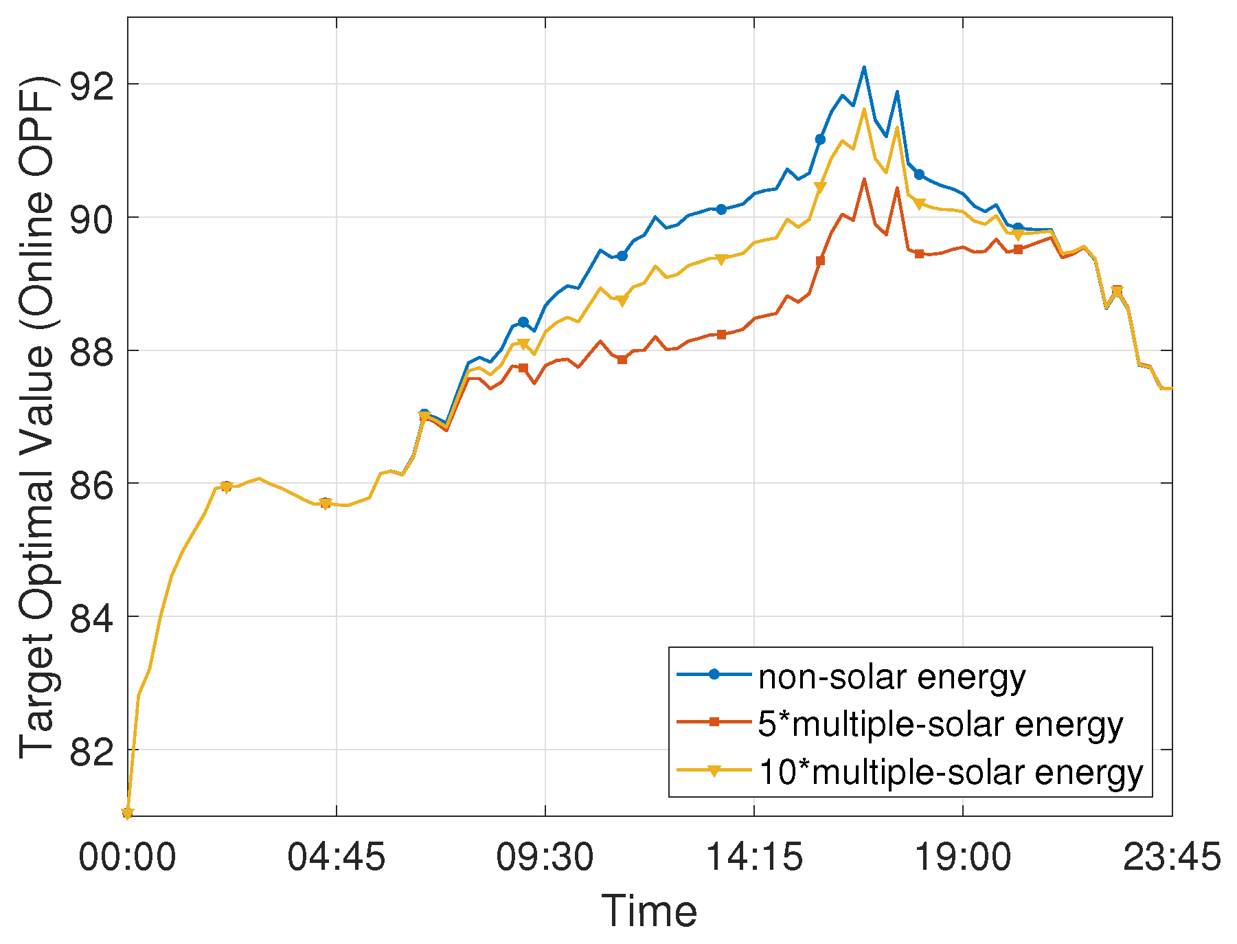
Under the time-varying load and solar power output given in Figure 6, we adopt the distributed online ADMM to solve the real-time optimal power flow. Figure 9 describes the convergence of the optimal value of OPF obtained by the algorithm over time under the background of no solar power access, 5 solar access points and 10 solar access points, as given in Figure 1b. The calculation example starts from 00:00. It is worth noting that within the initial hour, the algorithm needs to reach convergence within a certain period of time, that is, the optimal running state. In Figure 9, an obvious rising phase can be obtained. Obviously, due to the access of the high load side, the power input needs to climb to reach the balance with the load. After that, the algorithm performance reaches the optimum at this time in the configuration without solar energy access, which is the blue curve in Figure 9. Since the objective function is a linear function of active power, it will change with the load, as shown in the load curve in Figure 6. In the configurations with 5 solar access points and 10 solar access points, the power output is obviously constrained by the solar access point.
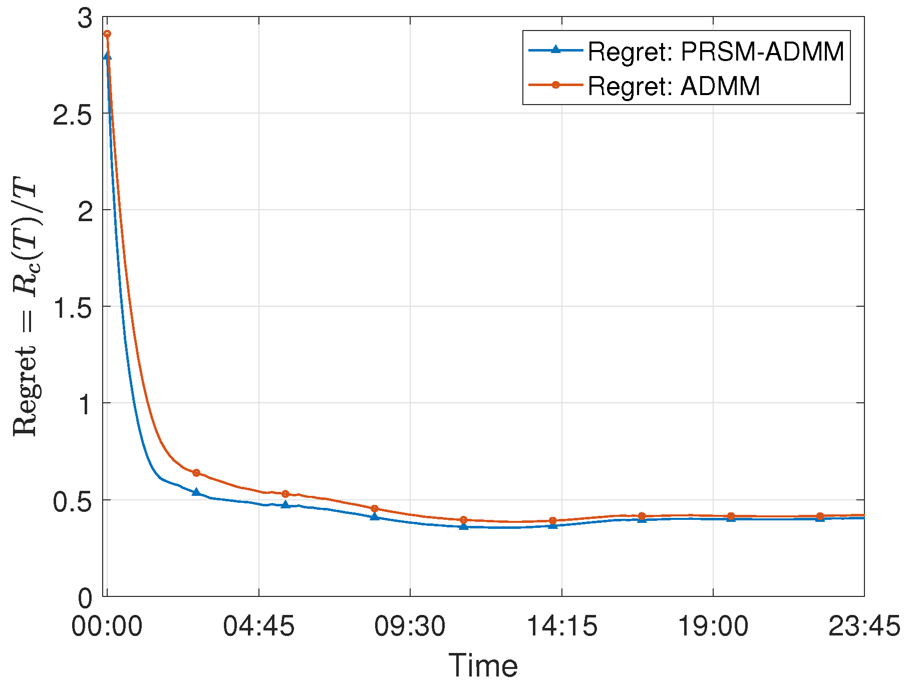
Finally, we evaluate the convergence performance of our distributed online ADMM for solving the real-time OPF problem. The algorithm makes the optimal decision for each time slot t to understand the instantaneous system state and minimizes the regret given in (22), as shown in Figure 10. In that, two versions of ADMM show very fine distinctions; PRSM-ADMM can approach convergence on a shorter time slot t and may play a greater advantage in solving online problems. It is particularly easy to see the algorithm has an obvious convergence lower bound on the time series, which verifies the good performance of the algorithm in the online case.
As a summary, we discuss the results and performance of the algorithm on online data. The algorithm has real-time calculation results for online data and can quickly reach the lower bound of regret.

6. Conclusions

This paper proposes a distributed control method for the OPF with renewables, which relies on SDP relaxation due to its nonconvexity. In summary, this work is split into two parts. First, based on the Lagrangian duality and ADMM, the method proposed is realized by solving the dual problem of the original OPF, in which the Lagrangian multipliers of the power flow equation are copied to each sub-area instead of the boundary coupling equation. Second, this distributed control method is extended to solving the dynamic OPF with renewables in an online fashion, which determines the current OPF value in each time slot, and achieves a regret bound within a limited time. Finally, the simulation results on the IEEE 30-bus system verify the high efficiency of the proposed distributed control method in solving both the static and dynamic OPF problems, and the online method can effectively avoid the violent fluctuations in conventional generator output coping with renewable’s rapid fluctuation in comparison with the offline algorithms.
Future works will mainly focus on addressing the two limitations of this study. First, since the algorithm of this paper considers the SDP based on AC power flow, it may be an interesting problem to extend to the large-scale AC-DC hybrid power model [41]. Second, for the dynamic, distributed OPF problem, although the experience proved that the SDP relaxation method has good interpretability for large-scale power grids, this method may not be the best match; it becomes an important task to seek new and more effective methods of analysis and design.

Author Contributions

S.W., L.P. and X.H. designed the distributed the OPF scheme, Y.S. and H.W. conceived the algorithm and application details, Y.Y. performed the simulations and prepared the manuscript. S.W. and H.W. led the project and research. All authors discussed the simulation results and approved the publication. All authors have read and agreed to the published version of the manuscript.

Funding

This work was supported in part by the Natural Science Foundation of Chongqing under Grant cstc2020jcyj-msxmX0057, and in part by the Science and Technology Research Program of Chongqing Municipal Education Commission under Grant KJZD-M202201204.

Institutional Review Board Statement

Not applicable.

Informed Consent Statement

Not applicable.

Data Availability Statement

Not applicable.

Conflicts of Interest

The authors declare no conflict of interest.

References

  1. Carpentier, J. Contribution to the economic dispatch problem. Bull. Soc. Fr. Electr. 1962, 3, 431–447. [Google Scholar]
  2. Madani, R.; Sojoudi, S.; Lavaei, J. Convex Relaxation for Optimal Power Flow Problem: Mesh Networks. IEEE Trans. Power Syst. 2015, 30, 199–211. [Google Scholar] [CrossRef]
  3. Kim, S.J.; Giannakis, G.B.; Lee, K.Y. Online Optimal Power Flow With Renewables. In Proceedings of the 2014 48th Asilomar Conference on Signals, Systems and Computers, Pacific Grove, CA, USA, 2–5 November 2014; pp. 335–360. [Google Scholar]
  4. Momoh, J.; Zhu, J. Improved interior point method for OPF problems. IEEE Trans. Power Syst. 1999, 14, 1114–1120. [Google Scholar] [CrossRef]
  5. Erseghe, T.; Tomasin, S. Power Flow Optimization for Smart Microgrids by SDP Relaxation on Linear Networks. IEEE Trans. Smart Grid 2013, 4, 751–762. [Google Scholar] [CrossRef]
  6. Lavaei, J.; Low, S. Zero Duality Gap in Optimal Power Flow Problem. IEEE Trans. Power Syst. 2012, 27, 92–107. [Google Scholar] [CrossRef] [Green Version]
  7. Sulc, P.; Backhaus, S.; Chertkov, M. Optimal Distributed Control of Reactive Power Via the Alternating Direction Method of Multipliers. IEEE Trans. Energy Convers. 2013, 29, 968–977. [Google Scholar] [CrossRef] [Green Version]
  8. Dall’Anese, E.; Zhu, H.; Giannakis, G. Distributed Optimal Power Flow for Smart Microgrids. IEEE Trans. Smart Grid 2013, 4, 1464–1475. [Google Scholar] [CrossRef] [Green Version]
  9. Erseghe, T. Distributed Optimal Power Flow Using ADMM. IEEE Trans. Power Syst. 2014, 29, 2370–2380. [Google Scholar] [CrossRef]
  10. Liao, C.Y.; Lin, W.; Chen, Y.M.; Chou, C.Y. A PV Micro-inverter With PV Current Decoupling Strategy. IEEE Trans. Power Electron. 2017, 32, 6544–6557. [Google Scholar] [CrossRef]
  11. Guo, J.; Hug, G.; Tonguz, O. A Case for Nonconvex Distributed Optimization in Large-Scale Power Systems. IEEE Trans. Power Syst. 2017, 32, 3842–3851. [Google Scholar] [CrossRef]
  12. Wang, Y.; Wu, L.; Wang, S. A Fully-Decentralized Consensus-Based ADMM Approach for DC-OPF with Demand Response. IEEE Trans. Smart Grid 2017, 8, 2637–2647. [Google Scholar] [CrossRef]
  13. Biagioni, D.; Graf, P.; Zhang, X.; Zamzam, A.S.; Baker, K.; King, J. Learning-Accelerated ADMM for Distributed DC Optimal Power Flow. IEEE Control Syst. Lett. 2022, 6, 1–6. [Google Scholar] [CrossRef]
  14. Jalali, M.; Kekatos, V.; Gatsis, N.; Deka, D. Designing Reactive Power Control Rules for Smart Inverters Using Support Vector Machines. IEEE Trans. Smart Grid 2020, 11, 1759–1770. [Google Scholar] [CrossRef] [Green Version]
  15. Turitsyn, K.; Sulc, P.; Backhaus, S.; Chertkov, M. Options for Control of Reactive Power by Distributed Photovoltaic Generators. Proc. IEEE 2011, 99, 1063–1073. [Google Scholar] [CrossRef] [Green Version]
  16. Boyd, S.P.; Parikh, N.; Chu, E.; Peleato, B.; Eckstein, J. Distributed Optimization and Statistical Learning via the Alternating Direction Method of Multipliers. Found. Trends Mach. Learn. 2011, 3, 1–122. [Google Scholar] [CrossRef]
  17. Biswas, P.P.; Suganthan, P.; Amaratunga, G.A. Optimal power flow solutions incorporating stochastic wind and solar power. Energy Convers. Manag. 2017, 148, 1194–1207. [Google Scholar] [CrossRef]
  18. Agalgaonkar, Y.P.; Pal, B.; Jabr, R. Stochastic Distribution System Operation Considering Voltage Regulation Risks in the Presence of PV Generation. IEEE Trans. Sustain. Energy 2015, 6, 1315–1324. [Google Scholar] [CrossRef] [Green Version]
  19. Xu, Y.; Hu, J.; Gu, W.; Su, W.; Liu, W. Real-Time Distributed Control of Battery Energy Storage Systems for Security Constrained DC-OPF. IEEE Trans. Smart Grid 2018, 9, 1580–1589. [Google Scholar] [CrossRef]
  20. Malekpour, A.; Pahwa, A. A Dynamic Operational Scheme for Residential PV Smart Inverters. IEEE Trans. Smart Grid 2017, 8, 2258–2267. [Google Scholar] [CrossRef]
  21. Gill, S.; Kockar, I.; Ault, G.W. Dynamic Optimal Power Flow for Active Distribution Networks. IEEE Trans. Power Syst. 2013, 29, 121–131. [Google Scholar] [CrossRef] [Green Version]
  22. Zhang, Y.; Gatsis, N.; Giannakis, G.B. Robust Energy Management for Microgrids With High-Penetration Renewables. IEEE Trans. Sustain. Energy 2012, 4, 944–953. [Google Scholar] [CrossRef]
  23. Gan, L.; Low, S.H. An Online Gradient Algorithm for Optimal Power Flow on Radial Networks. IEEE J. Sel. Areas Commun. 2016, 34, 625–638. [Google Scholar] [CrossRef]
  24. Tang, Y.; Dvijotham, K.; Low, S. Real-Time Optimal Power Flow. IEEE Trans. Smart Grid 2017, 8, 2963–2973. [Google Scholar] [CrossRef]
  25. Yan, Z.; Xu, Y. Real-Time Optimal Power Flow: A Lagrangian Based Deep Reinforcement Learning Approach. IEEE Trans. Power Syst. 2020, 35, 3270–3273. [Google Scholar] [CrossRef]
  26. Sayed, A.R.; Wang, C.; Anis, H.; Bi, T. Feasibility Constrained Online Calculation for Real-Time Optimal Power Flow: A Convex Constrained Deep Reinforcement Learning Approach. IEEE Trans. Power Syst. 2022, 1–13. [Google Scholar] [CrossRef]
  27. Trinklein, E.H.; Parker, G.G.; Robinett, R.D.; Weaver, W.W. Toward Online Optimal Power Flow of a Networked DC Microgrid System. IEEE J. Emerg. Sel. Top. Power Electron. 2017, 5, 949–959. [Google Scholar] [CrossRef]
  28. Zhu, X.; Han, X.; Yang, M.; Xu, Y.; Wang, S. Distributed online optimal power flow for distribution system. Int. J. Electr. Power Energy Syst. 2020, 120, 105970. [Google Scholar] [CrossRef]
  29. Pourbabak, H.; Alsafasfeh, Q.; Su, W. A Distributed Consensus-Based Algorithm for Optimal Power Flow in DC Distribution Grids. IEEE Trans. Power Syst. 2020, 35, 3506–3515. [Google Scholar] [CrossRef]
  30. Yang, L.; Luo, J.; Xu, Y.; Zhang, Z.; Dong, Z. A Distributed Dual Consensus ADMM Based on Partition for DC-DOPF With Carbon Emission Trading. IEEE Trans. Ind. Inf. 2020, 16, 1858–1872. [Google Scholar] [CrossRef]
  31. Fukushima, M. Application of the Alternating Direction Method of Multipliers to Separable Convex Programming Problems. Comput. Optim. Appl. 1992, 1, 93–111. [Google Scholar] [CrossRef]
  32. Von Luxburg, U. A tutorial on spectral clustering. Stat. Comput. 2007, 17, 395–416. [Google Scholar] [CrossRef]
  33. Hartigan, J.; Wong, M. Algorithm AS 136: A K-Means Clustering Algorithm. Ann. Appl. Stat. 1979, 28, 100–108. [Google Scholar] [CrossRef]
  34. Boyd, S.; Vandenberghe, L. Convex Optimization; Cambridge University Press: Cambridge, UK, 2004. [Google Scholar]
  35. Wang, H.; Banerjee, A. Online Alternating Direction Method. In Proceedings of the 29th International Conference on Machine Learning (ICML 2012), Edinburgh, UK, 26 June–1 July 2012; pp. 1119–1126. [Google Scholar]
  36. Kadkhodaie, M.; Christakopoulou, K.; Sanjabi, M.; Banerjee, A. Accelerated Alternating Direction Method of Multipliers. In Proceedings of the 21th ACM SIGKDD International Conference on Knowledge Discovery and Data Mining, Sydney, Australia, 10–13 August 2015; pp. 497–506. [Google Scholar]
  37. He, B.; Liu, H.; Wang, Z.; Yuan, X. Application of the Alternating Direction Method of Multipliers to Separable Convex Programming Problems. SIAM J. Control. Optim. 2014, 24, 1011–1040. [Google Scholar] [CrossRef] [PubMed] [Green Version]
  38. Ullah, Z.; Wang, S.; Radosavljević, J.; Lai, J. A Solution to the Optimal Power Flow Problem Considering WT and PV Generation. IEEE Access 2019, 7, 46763–46772. [Google Scholar] [CrossRef]
  39. Keyhani, A. Design of Smart Power Grid Renewable Energy Systems, 3rd ed.; Wiley Press: Hoboken, NJ, USA, 2019. [Google Scholar]
  40. Erseghe, T. A distributed approach to the OPF problem. EURASIP J. Adv. Signal Process. 2015, 2015, 1–13. [Google Scholar] [CrossRef] [Green Version]
  41. Meyer-Huebner, N.; Suriyah, M.; Leibfried, T. Distributed Optimal Power Flow in Hybrid AC–DC Grids. IEEE Trans. Power Syst. 2019, 34, 2937–2946. [Google Scholar] [CrossRef]
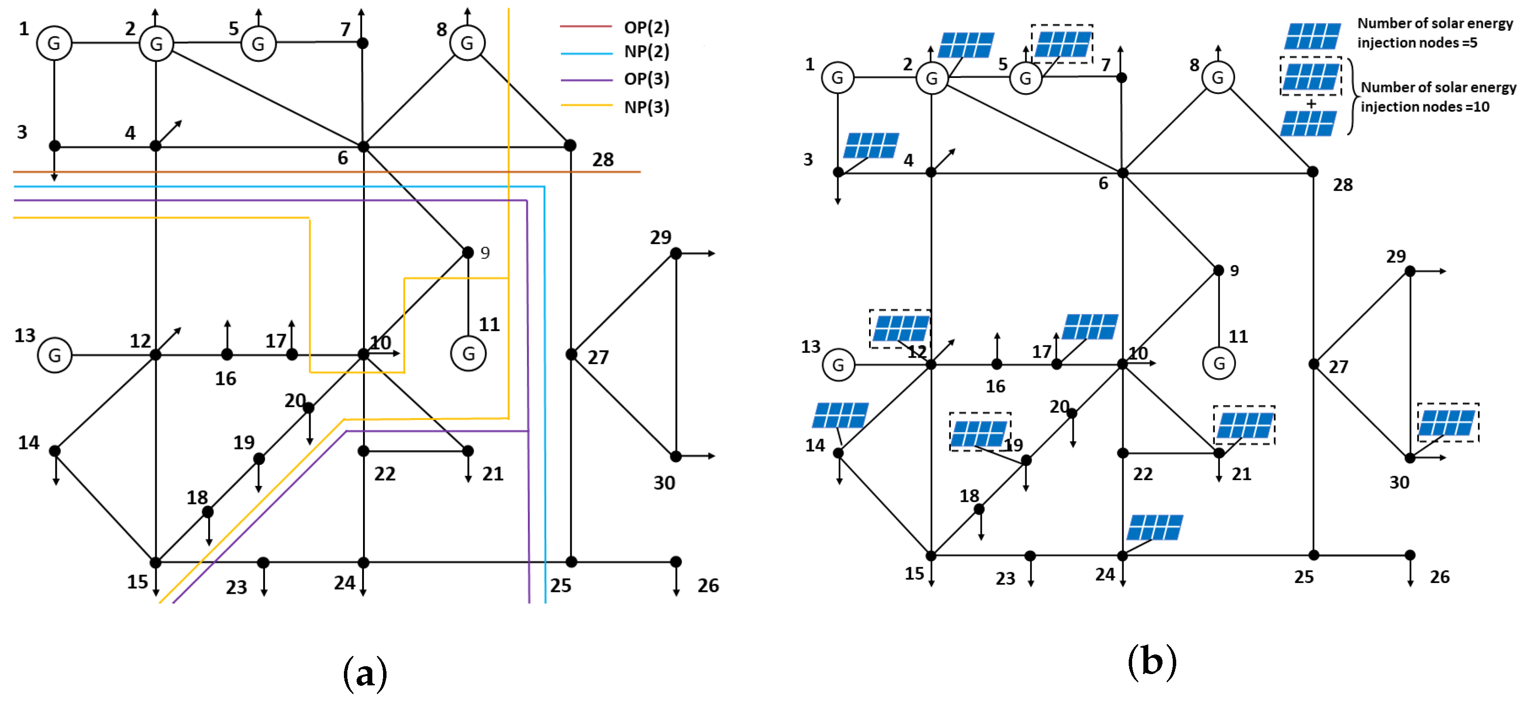
Figure 1. Test case for the IEEE 30-bus system. (a) Area partitioning cases; (b) Solar energy injection. (NP(2) and NP(3) are from [40]).
Energies 15 09525 g001
Figure 2. Iteration number v.s. dual penalty factor ρ for given residual accuracy. (NP(2) and NP(3) are from [40]).
Energies 15 09525 g002
Figure 3. Convergence of ADMM with different partitions. (a) Two regions, gap in objective value; (b) Three regions, gap in objective value. (NP(2)-Gap and NP(3)-Gap are from [40]).
Energies 15 09525 g003
Figure 4. Convergence of Lagrangian multiplier with different partitions. (a) Two regions, iterative performance; (b) Three regions, iterative performance. (NP(2)-LMC and NP(3)-LMC are from [40]).
Energies 15 09525 g004
Figure 5. Convergence of primal residual with different partitions. (a) Two regions, convergence performance; (b) Three regions, convergence performance. (NP(2)-PRC and NP(3)-PRC are from [40]).
Energies 15 09525 g005
Figure 6. Active/reactive load and solar power output data during 24 h (sampling every 15 min).
Energies 15 09525 g006
Figure 7. Cost comparison between the offline [30] and online algorithms solving the distributed OPF.
Energies 15 09525 g007
Figure 8. Conventional generation comparison between the offline [30] and online algorithms solving the distributed OPF.
Energies 15 09525 g008
Figure 9. Real-time optimal value of distributed ADMM under different solar configurations.
Energies 15 09525 g009
Figure 10. Regret bound of distributed online ADMM.
Energies 15 09525 g010
Table 2. Area partitioning cases for the IEEE 30-bus system.
Partitioning CaseSubregions
N P ( 2 ) [40] { 1 8 , 25 30 } & { 9 24 }
O P ( 2 ) ours. { 1 8 , 28 } & { 9 27 , 29 , 30 }
N P ( 3 ) [40] { 1 10 } & { 11 20 } & { 21 30 }
O P ( 3 ) ours. { 1 8 , 25 30 } & { 9 20 } & { 21 24 }
Table 3. Performance comparison among different partitions.
Partition OP ( 2 ) Ours NP ( 2 ) [40] OP ( 3 ) Ours NP ( 3 ) [40]
Iterations5274120153
Time (s)12410181451241
Public information8161440
Consensus variable15T31T25T76T
Coupling parameter0.61171.01950.75321.614
Gap99.57%99.89%99.35%99.22%
Publisher’s Note: MDPI stays neutral with regard to jurisdictional claims in published maps and institutional affiliations.