Active Power Cooperative Control for Wind Power Clusters with Multiple Temporal and Spatial Scales

Abstract

To improve the control of active power in wind power clusters, an active power hierarchical predictive control method with multiple temporal and spatial scales is proposed. First, the method from the spatial scale divides the wind power clusters into the cluster control layer, sub-cluster coordination layer and single wind farm power regulation layer. Simultaneously, from the temporal scale, the predicted data are divided layer by layer: the 15 min power prediction is deployed for the first layer; the 5 min power prediction is employed for the second layer; the 1 min power prediction is adopted for the third layer. Secondly, the prediction model was developed, and each hierarchical prediction was optimized using MPC. Thirdly, wind farms are dynamically clustered, and then the output power priority of wind farms is established. In addition, the active power of each wind farm is controlled according to the error between the dispatch value and the real-time power with feedback correction so that each wind farm achieves cooperative control with optimal power output. Finally, combined with the simulation of practical wind power clusters, the results show that the wind abandonment rate was reduced by 2.13%, and the dispatch of the blindness was overcome compared with the fixed proportional strategy. Therefore, this method can improve the efficiency of cooperative power generation.

1. Introduction

With the rapid development of wind power technology, the proportion of large-scale and clustered wind power in energy applications is gradually increasing [1]. The large-scale integration of a high percentage of wind power into the grid has put forward higher standards and requirements for the real-time balance of power generation, transmission and consumption of the power system [2]. However, with the vigorous promotion of high percentage wind power, its inherent intermittency, volatility and strong uncertainty are becoming increasingly prominent [3]. Wind power integration has a series of profound impacts on the development of power grid dispatching, posing a huge challenge to the balance of the power system [4]. Therefore, reasonable and optimal allocation of wind power output, improving the accuracy of wind power prediction, as well as how to control the active power of wind power clusters and develop an accurate wind farm output plan have become urgent issues to be solved. Nowadays, the method of wind turbine output power prediction using large-scale data information is a prerequisite and basis for solving this problem [5,6,7].

Many scholars have carried out research on different prediction models for the accuracy of wind power prediction [8,9,10]. There are various wind power prediction methods. Different algorithms have their own advantages and disadvantages, so the prediction errors are different. Reference [11] evaluated the past and present wind power prediction methods and looked into the future trends of wind power prediction methods. Reference [12] proposed combined prediction intervals by entropy weight based on the naive Bayes model to improve the wind power prediction performance. Reference [13] proposed a combined forecasting method for wind power prediction, which takes full use of the advantages of each model. Reference [14] selected different individual prediction models and used a weighted combination method to combine the individual predicted values to obtain the final predicted values, which effectively improved the prediction accuracy. Wind power clusters can achieve more stable wind power than the large fluctuations of individual wind farm power, so wind power cluster power prediction has a greater value [15]. Reference [16] effectively divides wind power clusters and establishes prediction models for different clusters, which reduces power prediction errors and improves the efficiency of modeling. Reference [17] proposes an active power control method for wind power clusters considering the prediction error, which reduces the power difference between cluster output and dispatch requirements due to the prediction error. Reference [18] was carried out using artificial neural networks. The results show that the proposed model may be better for fitting the actual curve of wind power. It shows the advantages of artificial neural networks in prediction. The accuracy of the above prediction model should be improved, but the prediction model is more complex and requires meteorological and other data. In fact, it is difficult to obtain meteorological data on smaller temporal scales in actual dispatch. Moreover, most wind farms can only obtain power data. At the same time, more complex prediction models can reduce the speed of forecasting and have a negative impact on ultra-short-term dispatching. In summary, the complexity of the prediction model needs to be considered in ultra-short-term dispatching. Above all, the genetic algorithm (GA)-improved BP neural network has higher accuracy and simple models in the ultra-short-term prediction process.

At present, a lot of fruitful research has been conducted by domestic and foreign scholars on cooperative control within wind power clusters. Research shows that model predictive control (MPC) theory has achieved good results in dealing with power systems containing wind power [19]. Reference [20] introduces MPC into hierarchical control for wind power clusters to improve wind power accommodation while ensuring system safety. In reference [21], a fixed-time region method was designed that considers the complete information of wind power prediction data. This makes the wind farm dynamic clustering results applicable not only to a certain moment of time but also to the selected time interval, laying the foundation for the realization of active power control of wind power clusters. Reference [22] proposed a double-stage hierarchical adaptive neuro-fuzzy inference system prediction model. It is introduced into the hierarchical control of wind power clusters. The results prove that it can effectively improve the prediction accuracy and wind power accommodation level. Reference [23] used an improved continuous method model for wind power prediction and introduced hierarchical control of wind power clusters to enable cooperative control of each wind farm, which improved the coordination of wind farm energy storage. Reference [24] contributes to the active output allocation of wind farms by using distributed model predictive control theory to analyze the error distribution characteristics of wind farms. Reference [25] introduced MPC into the coordination of wind farm power to solve the problem of faults caused by reactive power deficiency. Reference [26] proposed a design and optimization method for wind turbine blades, which solved the coupling problem of blade structure strength and improved the power generation efficiency of wind turbines. Reference [27] proposed a new wind power dispatch optimization scheme based on MPC, which is important for wind farm tracking and dispatch plans. In this approach, a combined prediction model based on variance-covariance variable weights is used to provide prediction information for dispatch and maximizing the wind power generation. The analysis of the above literature reveals that none of the relevant literature considers specific methods of wind farm coordination at different temporal scales when achieving coordinated cooperation between different layers of the wind power cluster. At the same time, the above literature does not mention the impact of wind power on the dispatch. The premise to ensure the smooth progress of the above control is that wind power prediction can effectively cooperate with wind power cluster control.

To further improve the accuracy of the wind power cluster tracking the dispatch plan, rationalizing the wind farm output and giving full play to the advantages of wind power have a very high economic value and social benefits. In this paper, an active power hierarchical predictive control model in wind power clusters is proposed by taking advantage of GA-BP and MPC theories. The method can be gradually optimized in temporal and spatial scales to improve collaborative control accuracy. Progressive optimization of wind power prediction information on the temporal scale to reduce prediction errors. At the spatial scale, the wind power clusters are controlled layer by layer, and each layer is adjusted separately on a rolling optimization. The effectiveness of the method is validated by conducting a simulation study with the actual measured data from a wind power base in China.

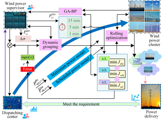
2. Active Power Hierarchical Predictive Control for Wind Power Clusters Based on MPC

In order to realize the cooperative power output among wind farms in a wind power cluster, this paper proposes an active power cooperative control method for wind power clusters with multiple temporal and spatial scales. The control block diagram of the active power stratification predictive control approach is shown in Figure 1. The optimization modes are selected according to the size of the planned value issued by the dispatch center and the predicted value of wind power: when the dispatched value is larger than the predicted value, the operation is in the planned power mode. On the contrary, the operation is in maximum power mode. The feedback correction corrects the next step of prediction and optimization, making it closer to the actual basis for closed-loop rolling optimization.

Different wind farms within a wind power cluster are located in different geographical environments and have different wind speed resources, so different wind farms have different outputs from each other [28]. In order to reasonably arrange wind farm power generation, this paper combines MPC to achieve active power hierarchical predictive control of a wind power cluster. An active power stratification predictive control strategy for a wind power cluster with multiple temporal and spatial scales is shown in Figure 2. MPC is an optimization-based control algorithm, and rolling optimization is an important part of it. Through the idea of hierarchical control, the wind power cluster is divided into three layers from the spatial scale, each of which includes the operating blocks of the MPC. From the multiple temporal scapes, each layer used different temporal scales of wind power prediction data. The 15 min ultra-short-term wind power prediction is deployed for the cluster control layer. The 5 min ultra-short-term wind power prediction is employed for the sub-cluster coordination layer. The 1 min ultra-short-term wind power prediction is adopted for the single wind farm power regulation layer. Through layer-by-layer refinement control and reasonable allocation of wind farm output, the problem of inaccurate planning caused by wind power prediction errors can be reduced.

In order to improve wind farm generation efficiency and wind energy utilization, the cluster layer control model contains two modules for the dynamic clustering of wind farms and optimization of cluster output. This layer is based on 15 min ultra-short-term wind power prediction results by combining with wind power change trends. What is more, it establishes wind farms for dynamic clustering and lays the foundation for post-layer control. The control variable of this layer is the sub-cluster output power, and the rolling optimization is executed every 15 min. The optimization time domain is set to 45 min. The first optimization result is executed each time. The sub-cluster coordination layer model uses the single wind farm output power as the control variable and is based on the information of the 5 min active power prediction data. The rolling period is 5 min, and three rolling optimizations are executed. The optimization time domain is set to 15 min to optimize the output power of the upper layer. Meanwhile, comparing the magnitude relationship between the predicted and dispatched values lays the foundation for a single wind farm power regulation layer. It is further refined on the basis of the previous layer. The time resolution of ultra-short-term wind power prediction is 1 min. The rolling optimization period and time domain is set to 1 min. Finally, it develops a priority set of wind power output based on wind farm dynamic grouping.

3. Active Power Prediction for Wind Power Clusters Based on GA-BP

An ultra-short-term active power prediction model based on GA-BP is proposed. BP neural networks are feedforward networks with a multi-layer structure, where the hidden layers can also be multi-layered. Figure 3 shows the structure of the BP neural network. Although BP neural networks are simple, the prediction accuracy will exceed complex prediction methods in ultra-short-term power prediction. In this paper, we mainly predict the wind power at 1, 5 and 15 min. In summary, a GA-BP neural network is reasonable. Therefore, it is reasonable to use GA-BP neural networks for ultra-short-term prediction of the output power of each wind farm within the wind power cluster.

3.1. GA-BP Neural Network

A GA-BP neural network is based on a BP neural network. In order to improve the accuracy of its model, GA is applied to overcome the disadvantage that the model is prone to local traps due to the randomly given weights and thresholds of the BP neural network. GA has excellent global search ability, so it is selected to optimize the initial weights and thresholds of the BP neural network to improve the convergence speed of the network. The BP neural network is also improved in terms of prediction accuracy. The simplicity of the model gives it an advantage in ultra-short-term wind farm dispatch due to its faster prediction speed relative to complex prediction models in 1, 5 and 15 min wind power prediction.

3.2. Wind Power Dispatch Analysis on Temporal Scale

The GA-BP neural network can provide reasonable wind power prediction data for 1, 5 and 15 min ultra-short-term dispatch. Its reasonableness is reflected in the fact that the dispatching process can accept dispatching instructions faster so that it can take the regulation power determined by the latest predicted data to achieve the purpose of meeting the dispatching plan. The wind power dispatch analysis on a temporal scale is shown in Figure 4.

As can be seen from Figure 4, the wind farm needs wind power predictions for the dispatch center to issue a new dispatch instruction in the case where issuing and determining the dispatch instructions and uploading the predicted data is ignored [29]. The wind farm can only follow the dispatch instructions of the previous time period to produce power during this time. Since the prediction accuracy is higher the closer to the prediction point, the average accuracy of the last time period dispatching instruction is not as good as the immediate dispatching instruction issued by the real-time prediction. In theory, the larger the proportion of the total time for immediate dispatch instructions to power output, the higher the efficiency of wind energy utilization. It is of great significance to shorten the wind power predictive time to improve the efficiency of wind power cluster generation [30].

3.3. Ultra-Short-Term Active Power Prediction Based on GA-BP

The flow chart of the predicted ultra-short-term wind power output using the GA-BP neural network is shown in Figure 5. The input data selected for this paper are: wind speed, wind direction of the wind tower, historical power data of the wind farm and NWP weather data. We group the above datasets and use the first 60% of them as the model training set, the middle 30% as the validation set and the last 10% as the test set. The data were normalized to eliminate the effect of the variation in the installed capacity of different wind farms. The predicted time domain is set to 24 h.

4. Hierarchical Predictive Control Multi-Objective Rolling Optimization Model

MPC is based on the construction of the controlled object; finding the optimal solution to reach the control objective by rolling optimization [31,32,33]. In the next control time domain, the feedback information obtained is used to perform a new round of optimization. Figure 6 shows a diagram of rolling optimization in MPC. Rolling optimization only performs the optimization process of the current optimal control variable [34].

4.1. Dynamic Clustering of Wind Farms

With the increase in installed wind power capacity, large-scale wind energy access to the grid has formed a trend. The volatility of wind energy will form a major disturbance to the power system [35]. Based on the ultra-short-term wind power active power predicted data, wind farms are classified according to the changes in active power that will occur in the future and wind farms with the same trend of change are grouped into the same category. Therefore, it is possible to determine the trend of output power variation of the wind farm with the closest variation pattern using the active power predicted by the GA-BP neural network. Every 45 min is used as a time interval to dynamically group the power variation of wind farms for 24 h. This approach not only reflects useful information from wind power comprehensively but also can track the wind resource changes over time, which makes the application of dynamic groups more universal and the results more accurate.

Using the 24 h active output power prediction information of the wind farm obtained from the prediction model, the time resolution is set to 15 min. The rolling optimization is executed every 15 min. The set of trend changes in output power for the next 45 min is combined with the prediction moment. In order to distinguish the small range fluctuation during continuous rising or falling, we calculate the difference between the maximum and minimum values of the wind farm trend judgment power sequence. After several experiments and analyses, the threshold value is set to one percent of the installed capacity of wind farms when the installed capacity of wind farms is within 150 MW; the threshold value is set to 5 MW when the installed capacity of wind farms is greater than or equal to 150 MW, as shown in Equations (1)–(4).

$${\mathsf{\Omega }}_{P_i}=\left[P_{i,t}^{\mathrm{for}},P_{i,t+1}^{\mathrm{for}},P_{i,t+2}^{\mathrm{for}},P_{i,t+3}^{\mathrm{for}}\right]$$

(1)

$${\gamma }_i=sign\left(P_{i,t+1}^{\mathrm{for}}-P_{i,t}^{\mathrm{for}}\right)+sign\left(P_{i,t+2}^{\mathrm{for}}-P_{i,t+1}^{\mathrm{for}}\right)+sign\left(P_{i,t+3}^{\mathrm{for}}-P_{i,t+2}^{\mathrm{for}}\right)$$

(2)

$$\mathit{M}=max\left({\mathsf{\Omega }}_{P_i}\right)-min\left({\mathsf{\Omega }}_{P_i}\right)$$

(3)

$$\eta =\left\{\begin{array}{cc}{P}_i^N/100,\hfill & P_i^N<150\mathrm{MW}\hfill \\ 5\mathrm{MW},\hfill & P_i^N\ge 150\mathrm{MW}\hfill \end{array}\right.$$

(4)

where ${\mathsf{\Omega }}_{P_i}$ is the power trend set for the next 45 min, t is the current time, $P_{i,t}^{\mathrm{for}}$ is the prediction power of wind farm i at t time, $P_{i,t+1}^{\mathrm{for}}$ is the predictive power for 15 min, $P_{i,t+2}^{\mathrm{for}}$ is the predictive power for 30 min, $P_{i,t+3}^{\mathrm{for}}$ is the predictive power for 45 min, ${\gamma }_i$ is the wind power variation trend factor, sign(x) is a function that takes the sign of a certain number (positive or negative) and is used to determine the trend of wind power variation, $\mathit{M}$ is the difference between the maximum and minimum values of the wind farm trend judgment power sequence, $\eta$ is the threshold value and $P_i^N$ is the installed capacity of wind farm i. When $M\le \eta$, it is defined as the transitional fluctuation group. When $M=0$, it is defined as the smooth group. When x > 0, sign(x) = 1; when x = 0, sign(x) = 0; when x < 0, sign(x) = −1. From Equation (2), it can be calculated that max (${\gamma }_i$) = 3, min (${\gamma }_i$) = −3. As a result, the trend of wind farm power can be determined. When ${\gamma }_i=0$, it means that the value of sign(x) will continue to be equal to 0 in the next 45 min; therefore, wind power trends remain unchanged, $P_{i,t+1}^{\mathrm{for}}-P_{i,t}^{\mathrm{for}}=0$, and it is defined as the smooth group. When max (${\gamma }_i$) = 3, it means that the value of sign(x) will continue to be equal to 1 for the next 45 min; when the wind power prediction series show an increase, $P_{i,t+1}^{\mathrm{for}}-P_{i,t}^{\mathrm{for}}>0$, it is defined as the uphill group. When min (${\gamma }_i$) = −3, it means that the value of sign(x) will continue to be equal to −1 in the next 45 min; when the wind power prediction series show a decrease, $P_{i,t+1}^{\mathrm{for}}-P_{i,t}^{\mathrm{for}}<0$, it is defined as the downhill group. When $-3<{\gamma }_i<3$, it means that the wind power is not monotonically increasing or decreasing. At this time, the wind power prediction series shows fluctuation, which is defined as the oscillating group.

$$\Delta \sigma =P_{i,t+1}^{\mathrm{for}}-P_{i,t}^{\mathrm{for}}$$

(5)

where $\Delta \sigma$ is the trend of power change.

According to Equation (5), the wind farm oscillation group can be further classified as two kinds of groups, as demonstrated in Equations (6) and (7).

(1)

First uphill then downhill group.

$$\left\{\begin{array}{c}\Delta {\sigma }_{\Delta t}>0\hfill \\ \Delta {\sigma }_{\Delta t+1}<0\hfill \end{array}\right.$$

(6)

(2)

First downhill then uphill group.

$$\left\{\begin{array}{c}\Delta {\sigma }_{\Delta t}<0\hfill \\ \Delta {\sigma }_{\Delta t+1}>0\hfill \end{array}\right.$$

(7)

The problem of bias caused by incomplete information on the future output power of wind farms is addressed by using a single point value as the basis for determining the output power state at a certain moment. This paper designs a power change trend factor as the basis of the judgment of wind farms based on the power change trend factor, taking into account output power information of wind power clusters in a fixed time window instead of a single time section. The dynamic clustering results are applicable to all wind farms in the selected time period. The dynamic clustering criterion for wind farms is shown in

Table 1. Wind power dynamic clustering criterion.

Number	Criteria	Group Type
0	${\gamma }_i=0$ or $M=0$	Smooth group
1	${\gamma }_i=3,M>\eta$	Uphill group
2	${\gamma }_i=-3,M>\eta$	Downhill group
3	$\left\{\begin{array}{c}\Delta {\sigma }_{\Delta t}>0\hfill \\ \Delta {\sigma }_{\Delta t+1}<0\hfill \end{array}\right.$	First uphill then downhill group
4	$\left\{\begin{array}{c}\Delta {\sigma }_{\Delta t}<0\hfill \\ \Delta {\sigma }_{\Delta t+1}>0\hfill \end{array}\right.$	First downhill then uphill group
5	$M\le \eta$	Transitional fluctuation group

. Figure 7 shows the process of a wind farm dynamic cluster. The characterization of dynamic wind power grouping is shown in

Table 2. Characterization of dynamic wind power grouping.

Group Type	Characterization
Smooth group	No change in output power trend
Uphill group	The output power shows an upward trend and is able to complete the increased power command
Downhill group	The output power shows a downward trend and is able to complete the power reduction command
Oscillating group	The output power shows a trend of rising then falling, falling then rising
Transitional fluctuation group	The output power fluctuates up and down, easily causing control errors

.

4.2. Cluster Layer Control Model

There are two rolling optimization objectives for the cluster layer, which are to minimize fluctuations in wind power output and to achieve maximum power output from wind power clusters. Adjusting the total dispatch plan of the wind power cluster by receiving the dispatch plan values and comparing them with the wind power predicted values within 15 min. The sub-cluster dispatch plan is issued based on the comparison results. Its objective function is shown in Equation (8).

$$\min J_{\mathrm{clu}}=\sum _{k=1}^T\sum _{j=1}^m{\alpha }_j\left[{\lambda }_{j_1}{\left(P_{ji,t+\Delta t}^{\mathrm{opt}}-P_{ji,t}^{\mathrm{act}}\right)}^2+{\lambda }_{j_2}{\left(P_{ji,t+\Delta t}^{\mathrm{opt}}-{\overline{P}}_{ji,t+\Delta t}^{\mathrm{opt}}\right)}^2\right]$$

(8)

where m is the number of sub-cluster types, T is the predicted time domain, ${\alpha }_j$ is the weight of the j sub-cluster, ${\lambda }_{j_1}$ is the weight for suppressing fluctuations in wind power output, ${\lambda }_{j_2}$ is the weight to maximize the cluster out, $P_{ji,t+\Delta t}^{\mathrm{opt}}$ is the power value of wind farm i in j cluster at $t+\Delta t$ time, $P_{ji,t}^{\mathrm{act}}$ is the actual power value at t moment and ${\overline{P}}_{ji,t+\Delta t}^{\mathrm{opt}}$ is ultra-short-term wind power prediction for 15 min. In the cluster layer, the future 1 h plan value is optimized each time. The resolution is set to 15 min, so T = 4. Only the results at k = 1 are taken for rolling optimization each time.

Equations (9)–(12) are the constraints:

(1)

Wind power cluster output climbing limit.

$$\mid \sum _{j=1}^m\sum _{i=1}^n{P}_{ji,t+\Delta t}^{\mathrm{opt}}-\sum _{j=1}^m\sum _{i=1}^n{P}_{ji,t}^{\mathrm{act}}\mid \le {\overline{D}}_{\mathrm{clu}}{P}_{\mathrm{clu}}^N$$

(9)

where n is the number of wind farms in each sub-cluster, ${\overline{D}}_{\mathrm{clu}}$ is the climbing rate limit for the layer (15 min) and $P_{\mathrm{clu}}^N$ is the sum of the installed capacity of all wind farms within the wind cluster.

(2)

Wind farm output climbing limit.

$$\mid P_{ji,t+\Delta t}^{\mathrm{opt}}-P_{ji,t}^{\mathrm{act}}\mid \le {\overline{D}}_{ji}{P}_{ji}^N$$

(10)

(3)

Limitation of wind farm output.

$$P_{ji}^{\min }\le P_{ji,t+\Delta t}^{\mathrm{opt}}\le {\overline{P}}_{ji,t+\Delta t}^{\mathrm{for}}\le P_{ji}^N$$

(11)

(4)

Wind power cluster dispatch plan tracking constraints.

$$\sum _{j=1}^m\sum _{i=1}^n{P}_{ji,t+\Delta t}^{\mathrm{opt}}=P_{\mathrm{sys},t+\Delta t}^{\mathrm{dis}}$$

(12)

where $P_{ji}^{\min }$ is the minimum output power of wind farm i in the j cluster, $P_{ji}^N$ is the installed capacity of wind farm i in the j cluster and $P_{\mathrm{sys},t+\Delta t}^{\mathrm{dis}}$ is the value of the wind power cluster power dispatch plan.

Through the MPC rolling optimization, the output power of each sub-cluster within the cluster is shown in Equation (13). This cluster rolling optimization result is used as the target value for each sub-cluster in the sub-cluster coordination layer.

$${\tilde{P}}_{j,t+\Delta t}^{\mathrm{opt}}=\sum _{i=1}^n{P}_{ji,t+\Delta t}^{\mathrm{opt}}$$

(13)

where ${\tilde{P}}_{j,t+\Delta t}^{\mathrm{opt}}$ is the output power of each wind farm in the cluster.

4.3. Sub-Cluster Coordination Layer Model

This layer is to realize the requirement of tracking the power grid dispatching commands. Comparing the dispatch instruction of the wind farm with the actual output value at the previous moment, the difference is the wind power output value that needs to be adjusted [36], as demonstrated in Equation (14). According to the wind power adjustment value, the output power priority set of wind farms responding to the changing characteristics of wind power in different time periods is determined by realizing the cooperative power output among wind farms in the wind power cluster and achieving the requirement of tracking the grid dispatching command.

$$\Delta P=P_{\mathrm{WFC}}^{dis}(t+1)-P_{\mathrm{WFC}}^{\mathrm{real}}\left(t\right)$$

(14)

where $P_{\mathrm{WFC}}^{dis}(t+1)$ is the dispatch command for the wind farm at t + 1 time, and $P_{\mathrm{WFC}}^{\mathrm{real}}\left(t\right)$ is the actual output value of the wind farm at t time.

(1)

The amount of dispatching changes $\Delta P>0$.

This situation means that system dispatching requires the wind cluster to generate more power at the next moment. At this time, it is necessary to regulate the output of wind farms with an increasing trend in output power within the wind power cluster, giving priority to the uphill group and the first uphill then downhill group.

(2)

The amount of dispatching changes $\Delta P<0$.

This situation means that system dispatching requires the wind cluster to generate less power at the next moment. At this time, it is necessary to arrange the wind farm output in the wind power cluster with decreasing active power, giving priority to the downhill group and the first downhill cluster then uphill group.

(3)

The amount of dispatching changes $\Delta P=0$.

This situation means that system dispatching requires the wind cluster to maintain power stability at the next moment. At this time, it is necessary to regulate the output of wind farms with a smooth trend of output active power within the wind power cluster, giving priority to the smooth group.

This layer model has the main objectives of tracking the planned value of the sub-cluster, suppressing the active power fluctuations and maximizing the output power. This layer considers ultra-short-term wind power predicted values at a 5 min resolution. The rolling cycle is 5 min, optimizing the output power for the next 15 min. It performs three optimizations between two optimization moments in the cluster layer. The initial single wind farm dispatching values are compared with the information of the 5 min ultra-short-term predicted data, and then the dispatch plan results are distributed to each wind farm to develop the initial single wind farm dispatching plan values. The objective function is demonstrated in Equation (15).

$$\begin{array}{c}\min J_{\mathrm{wfs}}=\hfill \\ {\displaystyle \sum _{k=1}^T}\left\{{\displaystyle \sum _{i=1}^n}\left[{\left(P_{i,t+\Delta t}^{\mathrm{opt}}-P_{i,t}^{\mathrm{act}}\right)}^2+{\left(P_{i,t+\Delta t}^{\mathrm{opt}}-{\widehat{P}}_{ji,t+\Delta t}^{\mathrm{opt}}\right)}^2\right]\right.\hfill \\ +\left.{\left({\displaystyle \sum _{i=1}^n}{P}_{i,t+\Delta t}^{\mathrm{opt}}-{\tilde{P}}_{j,t^{\prime }+\Delta t^{\prime }}^{\mathrm{opt}}\right)}^2\right\}\hfill \end{array}$$

(15)

where ${\stackrel{⌢}{P}}_{ji,t+\Delta t}^{\mathrm{for}}$ is the ultra-short-term wind power prediction for 5 min, ${\tilde{P}}_{j,t^{\prime }+{\Delta t}^{\prime }}^{\mathrm{opt}}$ is the planned value sent from the cluster layer to the sub-cluster layer, $t^{\prime }$ and $\Delta t^{\prime }$ correspond to the cluster layer moment and time difference and $\Delta t$ is 5 min.

Equations (16)–(19) are the constraints:

(1)

Wind power cluster output climbing limit.

$$\mid \sum _{j=1}^m\sum _{i=1}^n{P}_{ji,t+\Delta t}^{\mathrm{act}}-\sum _{j=1}^m\sum _{j=1}^n{P}_{ji,t}^{\mathrm{act}}\mid \le {\stackrel{⌢}{D}}_{\mathrm{clu}}{P}_{\mathrm{clu}}^N$$

(16)

where ${\stackrel{⌢}{D}}_{\mathrm{clu}}$ is the sub-cluster climbing rate limit.

(2)

Wind farm output climbing limit.

$$\mid P_{i,t+\Delta t}^{\mathrm{opt}}-P_{i,t}^{\mathrm{act}}\mid \le {\stackrel{⌢}{D}}_i{P}_{\mathrm{i}}^N$$

(17)

where ${\stackrel{⌢}{D}}_i$ is the wind farm climbing rate limit (5 min), and $P_i^N$ is the installed capacity of wind farm i.

(3)

Limitation of wind farm output.

$$P_i^{\min }\le P_{i,t+\Delta t}^{\mathrm{opt}}\le {\stackrel{⌢}{P}}_{i,t+\Delta t}^{\mathrm{for}}\le P_i^N$$

(18)

(4)

Wind farm cluster scheduling plan tracking constraints.

$$\sum _{i=1}^n{P}_{i,t+\Delta t}^{\mathrm{opt}}\le {\tilde{P}}_{i,t^{\prime }+{\Delta t}^{\prime }}^{\mathrm{opt}}$$

(19)

where $P_i^{\min }$ is the minimum output power of wind farm i, and $P_i^N$ is the installed capacity of wind farm i. The results obtained from the sub-cluster layer are sent down to the wind farms within the cluster to be used as tracking targets for the next layer.

4.4. Single Wind Farm Power Regulation Model

The wind farm receives the dispatch issued by the sub-cluster coordination layer every 5 min. The optimized time domain is 1 min, so T = 1. This layer is mainly used to adjust the wind farm itself with ultra-short-term wind power predicted values at 1 min resolution to improve the control accuracy, track the wind farm dispatching objectives and maximize the needs of system dispatching and to suppress wind power fluctuations as the main objectives, as demonstrated in Equation (20).

$$\min J_{\mathrm{wf}}={\left(P_{i,t+\Delta t}^{\mathrm{opt}}-P_{i,t}^{\mathrm{act}}\right)}^2+{\left(P_{i,t+\Delta t}^{\mathrm{opt}}-{\widehat{P}}_{i,t^{″}+{\Delta t}^{″}}^{\mathrm{opt}}\right)}^2$$

(20)

Equations (21)–(23) are the constraints:

(1)

Wind farm output climbing limit.

$$\left|P_{i,t+\Delta t}^{\mathrm{opt}}-P_{i,t}^{\mathrm{act}}\right|\le {\stackrel{⌢}{D}}_i{P}_i^N$$

(21)

(2)

Limitation of wind farm output.

$$P_i^{\min }\le P_{i,t+\Delta t}^{\mathrm{opt}}\le {\stackrel{⌢}{P}}_{i,t+\Delta t}^{\mathrm{for}}\le P_i^N$$

(22)

(3)

Wind farm cluster scheduling plan tracking constraints.

$$P_{i,t+\Delta t}^{\mathrm{opt}}\le {\stackrel{⌢}{P}}_{j,t^{″}+{\Delta t}^{″}}^{\mathrm{opt}}$$

(23)

where ${\widehat{P}}_{i,t^{″}+{\Delta t}^{″}}^{\mathrm{opt}}$ is the dispatch plans issued from the sub-cluster coordination layer, ${\widehat{P}}_{i,t+\Delta t}^{\mathrm{for}}$ is the predicted value of wind power (1 min) and ${\widehat{D}}_i$ is the single wind farm output climbing rate limit (1 min).

5. Simulation Study

5.1. GA-BP Neural Network Prediction Results

To validate the effectiveness of the proposed method in this paper, the wind power data of a wind power cluster from 1 February to 27 February 2021 are used as the training dataset; the actual measured wind power data are from 28 February 2021. The experimental dataset includes time series data of four different categories of wind speed, wind direction, temperature and wind power. The wind power cluster contains six wind farms with the installed capacity shown in

Table 3. Wind farm installed capacity.

Wind Farm Number	Installed Capacity (MW)
WF1	201
WF2	50
WF3	94
WF4	99
WF5	96
WF6	98.8

.

Figure 8 shows the wind farm power prediction curve. From Figure 8, it can be seen that the GA-BP neural network predicts the curve closest to the actual curve throughout the ultra-short-term wind power cluster power prediction, and the fluctuation trend follows the original power trajectory. Compared with the BP neural network prediction results, the proposed method has significantly improved the performance of power prediction. It can be seen that the GA-BP neural network is more advanced in wind power prediction and has higher prediction accuracy. Meanwhile, the reasonableness and accuracy of GA-BP in ultra-short-term wind power prediction are confirmed.

5.2. Analysis of Dynamic Grouping Results

There is no strict definition of a wind power cluster, but it can generally be summarized as a collection of several wind farms in close proximity to each other in terms of geographic location or electrical network structure with complementary relationships where the wind power clusters are integrated into the grid. On the one hand, it can achieve flexible control of the output power of wind power within the cluster, and on the other hand, it can make full use of wind resources to achieve friendly scheduling and control of output power. In this paper, the active power of wind farms is dynamically clustered according to the ultra-short-term power predicted data on 28 February 2021. Dynamic clustering of wind farms in a cluster is performed according to wind power dynamic clustering criterion and trends in wind power forecast data. The clustering results are shown in

Table 4. Results of wind farm dynamic cluster.

Time	WF1	WF2	WF3	WF4	WF5	WF6
00:00–00:45	2	3	4	2	2	2
00:45–01:30	2	2	2	3	3	2
01:30–02:15	2	1	2	1	4	4
02:15–03:00	2	1	2	1	0	4
03:00–03:45	2	0	3	3	0	1
03:45–04:30	4	3	3	2	0	1
04:30–05:15	1	0	4	3	0	1
05:15–06:00	4	2	1	4	0	2
06:00–06:45	1	0	4	1	4	3
06:45–07:30	4	1	3	1	1	4
07:30–08:15	1	2	2	1	3	1
08:15–09:00	2	1	1	3	4	2
09:00–09:45	4	1	2	2	1	2
09:45–10:30	2	1	1	2	1	5
10:30–11:15	4	2	1	1	4	2
11:15–12:00	2	2	2	3	2	1
12:00–12:45	4	5	3	2	4	4
12:45–13:30	1	5	4	1	4	1
13:30–14:15	1	2	3	3	3	1
14:15–15:00	4	4	4	2	3	4
15:00–15:45	2	4	4	4	4	1
15:45–16:30	2	1	3	4	3	1
16:30–17:15	4	1	3	2	4	5
17:15–18:00	1	1	1	1	4	1
18:00–18:45	1	1	1	1	1	2
18:45–19:30	1	1	4	1	3	2
19:30–20:15	1	3	3	1	1	2
20:15–21:00	1	4	1	2	2	2
21:00–21:45	1	2	1	3	4	2
21:45–22:30	1	2	2	3	2	2
22:30–23:15	1	1	1	1	2	2
23:15–24:00	1	3	2	1	4	2

.

During the normal operation of a wind farm, the active power is in constant change due to the uncertainty and randomness of the wind resource. Synchronous scheduling means that the dispatching command and the real-time power change trend are the same; asynchronous scheduling means that the dispatching command and the real-time power change trend are not the same [37]. Therefore, the wind farm output power sequence is regulated to ensure that the wind power tracks the grid dispatch commands.

When the predicted value of the wind farm output power lies above the dispatch plan value, the dispatch department needs to adjust the output power to achieve the power reduction. When the predicted value of active power is below the dispatch plan value, it is necessary to track the maximum output power and increase the output power regulation. In summary, the wind power output priority set is established, as shown in

Table 5. Wind power output priorities.

Mode	The Trend of Wind Power	Dispatch Directions	Dynamic Grouping of Output Power Priorities
Synchronous scheduling	Rise	Increase	1 > 3 > 0 > 2 > 4
	Decline	Decrease	2 > 4 > 0 > 3 > 1
Asynchronous scheduling	Rise	Increase	2 > 4 > 3 > 1 > 0
	Decline	Decrease	1 > 3 > 0 > 4 > 2

.

Figure 9 shows the wind power cluster power prediction and dispatch curve. When the system dispatch value is larger than the wind power prediction value, the wind farm runs the maximum power tracking mode. The dispatch department controls the active power of the wind power cluster to match the system dispatch command. When the system dispatch value is less than the wind power predicted value, the wind farms operate the planned power mode to control the coordinated power output of each wind farm in the wind power cluster.

From 09:15 to 13:30, the predicted value of the wind power cluster is larger than the dispatch value; the active power of the wind power cluster is in the planned power mode, so all wind farms in the wind power cluster need to be regulated to meet the dispatch plan value. During this period, power reduction regulation is required, and the optimal sequence of wind power clusters is the downhill group, first downhill then uphill group and smooth group. From 13:30 to 16:00, the predicted value of the wind power cluster is less than the dispatch value; the dispatch department issues an increase plan so that all wind farms in the wind power cluster are in the maximum active power mode. The optimal wind power cluster order to be regulated is the uphill group, first uphill then downhill group and smooth group. Specifically, the output power of each wind farm is coordinated against the cluster results to achieve the optimal output power of the wind power cluster.

5.3. Hierarchical Predictive Control Results

In this paper, the fixed proportion strategy is used for comparison with the hierarchical predictive control method. The core idea is to distribute the power according to the ratio size of each wind farm in the wind cluster to the total output power. Figure 10 shows the wind power cluster curve of the dispatch under different control strategies.

From Figure 10, it can be seen that the dispatching curve under the hierarchical control strategy can track the dispatching command to the maximum extent, but the fixed proportion method cannot fully respond to the cluster dispatching command. The analysis shows that the hierarchical control strategy allocates the dispatched power to the wind farm based on the predicted information. The fixed proportion method does not consider the predicted information so the wind farm dispatch power and wind farm predicted power mismatch. As a result, the wind farm energy storage coordination output and wind curtailment under the MPC-based strategy are higher.

Figure 11 shows the different control effects of wind power in a single wind farm under the two control methods. Relative to the overall effect, the hierarchical model control is more advanced to the fixed proportion method. Because of the dynamic clustering of wind farms in this paper, the hierarchical predictive control method can make full use of wind power prediction information to reasonably allocate power output among wind farms. For example, clustering results of the WF1 are in the smooth group from 15:15 to 17:45. Compared with the fixed proportional allocation method; the hierarchical predictive control makes full use of dynamic grouping information to bring the wind farm output curve closer to the dispatching plan. In the end, power generation and efficiency of wind energy utilization are improved. There is no tracking and dispatching curve for WF2 from 12:00 to 13:45. Because, at this time, the wind farms are divided into clusters that result in the transitional fluctuation group. The main goal of this type of sub-cluster is to suppress fluctuations. From 12:00 to 16:00, the main clustering results of WF5 are the downhill group and oscillating group so that the output curve decreases more gently and with lower volatility than the fixed proportion approach. From 6:00 to 9:45, the main clustering results of WF6 are the downhill group and transitional fluctuation group so that wind farms are in the planned power mode tracking dispatching power output. Therefore, the model given in the paper can achieve dynamic clustering of wind power clusters and real-time regulation of wind farm output through layer-by-layer refinement of power prediction information.

As can be seen in Figure 11, this method is effective in tracking the planned values throughout the period when the ultra-short-term wind cluster predicted power is less than the dispatched values. The MPC-based dispatching strategy is more advanced in dealing with wind power volatility. The MPC hierarchical control method tracks the dispatching plan values more smoothly, especially WF3, from 01:45 to 08:00, without large fluctuations. This is because the MPC dispatching method takes into account the predicted information of ultra-short-term wind power cluster power output on the one hand and effectively handles the continuous fluctuation of the wind cluster active power dispatching plan through rolling optimization and error feedback correction, on the other hand, to improve the stability of active power output. It shows that the MPC strategy can still achieve good results when dealing with non-stationary active power.

Under hierarchical predictive control, the wind farm output is optimized based on three links of predictive model control to track the grid dispatch plan values as the spatial and temporal scales are refined layer by layer. The accuracy of the tracking and dispatching plan is subsequently improved. For example, the WF4 output curve can effectively track the dispatch curve from 15:00 to 18:00. The error caused by the control effect is improved by the prediction information under the temporal scales, and the reasonable distribution of the wind farm output is realized.

5.4. Industrial Field Verification

In order to further analyze the effectiveness of the hierarchical predictive control method in coping with the active power control of wind power, this paper conducts industrial field validation of wind power clusters within a large wind power base. The industrial field application is shown in Figure 12.

As can be seen from Figure 12, this wind power cluster is in four regions, A, B, C and D, containing six wind farms with a total installed capacity of 638.8 MW. Areas A and D contain two wind farms, and areas B and C contain one wind farm. All wind turbines in the wind farm are of controllable power. The number of wind turbines included in each wind farm is 134, 25, 66, 55, 32 and 91, totaling 403 wind turbines. The method proposed in this paper is used to collaboratively control each wind farm in this wind power cluster with a control time horizon of 1 month. Figure 13 shows the comparison of the output power of the wind cluster under the two control methods.

From Figure 13, it can be seen that the proposed method of wind power cluster output power is better than the fixed proportion method. The successful field validation not only confirms the effectiveness of the cooperative control among the wind farms in the wind power cluster but also validates the advantages of the proposed method in improving the efficiency of wind power.

The wind abandonment rate is the percentage of wind power abandoned by the wind farm to the planned power generation in the statistical cycle, which measures the power generation efficiency of the wind turbine.

Table 6. Comparison of wind farm abandonment rates in different regions.

Area Number	Fixed Proportion Strategy (%)	Active Hierarchical Predictive Control (%)
A	7.43	5.23
B	6.54	5.08
C	8.49	6.03
D	5.80	3.37

shows the abandonment rates of wind farms in each region with different control strategies. It can be seen that the hierarchical predictive control method can reduce the abandoned wind rate. In general, the method proposed in this paper enables a coordinated distribution of the power output among the wind farms to improve the efficiency of wind power utilization while meeting the planned values of the wind power cluster dispatch center.

6. Conclusions

Based on the errors that occur between the predicted active power values of wind power clusters and the dispatch values and the serious imbalance in the long-term power distribution within wind farms, the ultra-short-term wind power prediction data are fully considered, and the active power hierarchical prediction control model with multiple temporal and spatial scales for a wind power cluster based on the MPC idea is proposed. The following conclusions are obtained.

(1) Application of MPC’s rolling optimization strategy for the wind cluster active control with continuous feedback correction using actual values. The GA-BP neural network is adopted in the prediction model to improve prediction accuracy. It is conducive to the development of more accurate wind power dispatching plans and the reduction in the wind power abandonment rate.

(2) Dynamic clustering of wind farms for wind power variation patterns in continuous time periods. The output power priority of wind farms within the cluster is established, which makes the active power dispatch mode of wind farms more reasonable. On the premise of meeting the grid dispatching plan, it can further effectively improve the ability of wind farms to make full use of wind energy resources and coordinate the power output of each wind farm to improve the efficiency of wind power cluster generation.

(3) A hierarchical predictive control model is used to overcome the problem of unreasonable distribution of active power output within traditional wind farms. The control accuracy is improved by layer-by-layer refinement from temporal and spatial scales. This reduces the impact of the wind power prediction error and wind power uncertainty on active power control.

(4) The advance in the hierarchical predictive control method for collaborative control among wind farms within a wind cluster is effectively demonstrated through industrial field application. This significantly increases the active output power of the wind power cluster, and the wind abandonment rate was reduced by 2.13%. This possesses practical engineering significance.

References

1. Du, G.; Zhao, D.M.; Liu, X. Research review on optimal scheduling considering wind power uncertainty. Proc. CSEE 2022, 10, 1–12. [Google Scholar]
2. Feng, Y.; Lin, H.Y.; Ho, S.L. Overview of wind power generation in China: Status and development. Reviews 2015, 50, 847–858. [Google Scholar] [CrossRef]
3. Zhang, B.M.; Chen, J.H.; Wu, W.C. A hierarchical model predictive control method of active power for accommodating large-scale wind power integration. Autom. Electr. Power Syst. 2014, 38, 6–14. [Google Scholar]
4. Kang, C.Q.; Yao, L.Z. Key scientific issues and theoretical research framework for power systems with high proportion of renewable energy. Autom. Electr. Power Syst. 2017, 41, 2–11. [Google Scholar]
5. Wang, Y.Q.; Gui, R.Z. A hybrid model for GRU ultra-short-term wind speed prediction based on tsfresh and sparse PCA. Energies 2017, 15, 7567. [Google Scholar] [CrossRef]
6. Xue, Y.S.; Yu, C.; Zhao, J.H.; Li, K.; Wu, Q.W.; Yang, G.Y. A review on short-term and ultra-short-term wind power prediction. Autom. Electr. Power Syst. 2015, 39, 141–151. [Google Scholar]
7. Li, Z.; Ye, L.; Zhao, Y.N. Short-term wind power prediction based on extreme learning machine with error correction. Prot. Control. Mod. Power Syst. 2016, 1, 1–8. [Google Scholar] [CrossRef] [Green Version]
8. Tascikaraoglu, A.; Uzunoglu, M. A review of combined approaches for prediction of short-term wind speed and power. Prot. Control. Mod. Power Syst. 2014, 34, 243–254. [Google Scholar] [CrossRef]
9. Ye, L.; Ren, C.; Zhao, Y.N.; Rao, R.S.; Teng, J.Z. Stratification analysis approach of numerical characteristics for ultra-short-term wind power forecasting error. Proc. CSEE 2016, 36, 692–700. [Google Scholar]
10. Wang, W.S.; Wang, Z.; Dong, C.; Liang, Z.F.; Feng, S.L.; Wang, B. Status and error analysis of short-term forecasting technology wind power in China. Autom. Electr. Power Syst. 2021, 45, 17–27. [Google Scholar]
11. Shahram, H.; Liu, X.L.; Lin, Z.; Saeid, L. A critical review of wind power forecasting methods—past, present and future. Energies 2020, 13, 3764. [Google Scholar]
12. Yang, X.Y.; Zhang, Y.F.; Ye, T.Z.; Su, J. Prediction of combination probability interval of wind power based on naive bayes. Energies 2020, 46, 1099–1108. [Google Scholar]
13. Li, Z.; Ye, L.; Dai, B.H.; Yu, Y.J.; Luo, Y.D.; Song, X.R. Ultra-short-term wind power prediction method based on IDSCNN-AM-LSTM combination neural network. High Volt. Eng. 2021, 46, 1–13. [Google Scholar]
14. Cheng, K.; Peng, X.S.; Xu, Q.Y.; Wang, B.; Liu, C.; Che, J.F. Short-term wind power prediction based on feature selection and multi-level deep transfer learning. High Volt. Eng. 2022, 48, 497–503. [Google Scholar]
15. Wang, B.; Liu, C.; Feng, S.L.; Qiu, G.; Meng, X.X.; Zhao, J.Y. Prediction method for short-term wind power based on wind farm clusters. High Volt. Eng. 2018, 44, 1254–1260. [Google Scholar]
16. Yang, Z.M.; Peng, X.S.; Lang, J.X.; Wang, H.Y.; Wang, B.; Liu, C. Short-term wind power prediction based on dynamic cluster division and BLSTM deep Learning method. High Volt. Eng. 2021, 47, 1195–1203. [Google Scholar]
17. Lu, P.; Ye, L.; Tang, Y.; Zhang, C.H.; Zhong, W.Z.; Sun, B.H.; Zhai, B.X.; Qu, Y.; Liu, X.Y. Multi-time scale active power optimal dispatch in wind power cluster based on model predictive control. Proc. CSEE 2019, 39, 6572–6582. [Google Scholar]
18. Huang, Q.H.; Wang, X. A forecasting model of wind power based on IPSO–LSTM and classified fusion. Energies 2022, 15, 5531. [Google Scholar] [CrossRef]
19. Ye, L.; Lu, P.; Zhao, Y.N.; Dai, B.H.; Tang, Y. Review of model predictive control for power system with large-scale wind power grid-connected. Proc. CSEE 2021, 41, 6181–6198. [Google Scholar]
20. Tang, Y.; Wang, Q.; Chen, N.; Zhu, L.Z. A dispatching method of active power in wind farm clusters considering probability distribution of forecasting errors. Proc. CSEE 2013, 33, 27–32. [Google Scholar]
21. Ye, L.; Zhang, C.H.; Tang, Y.; Sun, B.H.; Zhong, W.Z.; Lan, H.B.; Liu, H.; Li, P.; Huang, Y.H. Active power stratification predictive control approach for wind power cluster with multiple temporal and spatial scales coordination. Proc. CSEE 2018, 13, 3767–3780. [Google Scholar]
22. Liu, Q.; Fang, J.J.; Zhao, J.; Zhang, S.F.; Liu, D.C.; Chen, Y. Wind power dispatching control strategy based on DSA power prediction model. Electr. Power Constr. 2019, 40, 63–70. [Google Scholar]
23. Zheng, H.P.; Zeng, P.; Liu, X.Y.; Cheng, X.T.; Bo, L.M.; Yang, W.W.; Zhang, Y.F.; Cui, Y. Active power layered control strategy based on error feedforward prediction for multiple temporal and spatial scales wind power cluster. Electr. Power Constr. 2020, 41, 120–128. [Google Scholar]
24. Zhao, H.R.; Wu, Q.W.; Guo, Q.L. Distributed model predictive control of a wind farm for optimal active power control Part I: Clustering-based wind turbine model linearization. IEEE Trans. Sustain. Energy 2015, 6, 831–839. [Google Scholar] [CrossRef] [Green Version]
25. Ye, L.; Zhang, C.H.; Tang, Y. Hierarchical model predictive control strategy based on dynamic active power dispatch for wind power cluster integration. IEEE Trans. Power Syst. 2019, 6, 4617–4629. [Google Scholar] [CrossRef]
26. Xu, Y.Y.; Liu, P.F.; Irene, P.; He, G.H.; Alireza, H.; Hassan, G. Energy generation efficiency and strength coupled design and optimization of wind turbine rotor blades. J. Energy Eng. 2019, 145, 04019004. [Google Scholar] [CrossRef]
27. Zhao, H.R.; Wu, Q.W.; Wang, J.H. Combined active and reactive power control of wind farms based on model predictive control. IEEE Trans. Energy 2017, 32, 1177–1187. [Google Scholar] [CrossRef] [Green Version]
28. Sultana, W.R.; Sahoo, S.K.; Sukchai, S. A review on state of art development of model predictive control for renewable energy applications. Renew. Sustain. Energy Rev. 2017, 76, 391–406. [Google Scholar] [CrossRef]
29. Zhang, J.H.; Liu, Y.Q.; David, I. Optimal power dispatch within wind farm based on two approaches to wind turbine classification. Renew. Energy 2017, 102, 487–501. [Google Scholar]
30. Cui, Y.; Zeng, P.; Wang, Z.; Wang, M.C.; Zhang, J.T.; Zhao, Y.T. Multiple time scales scheduling strategy of wind power accommodation considering energy transfer characteristics of carbon capture power plant. Proc. CSEE 2021, 41, 946–961. [Google Scholar]
31. Zhang, X.S.; Yu, T.; Yang, B. A Random forest-assisted fast distributed auction-based algorithm for hierarchical coordinated power control in a large-scale PV power plant. IEEE Trans. Sustain. Energy 2021, 12, 2471–2481. [Google Scholar] [CrossRef]
32. Liu, X.J.; Feng, L.; Kong, X.B. A comparative study of robust MPC and stochastic MPC of wind power generation system. Energies 2022, 15, 4814. [Google Scholar] [CrossRef]
33. Ebrahimi, F.M.; Khayatiyan, A.; Farjah, E. A novel optimizing power control strategy for centralized wind farm control system. Renew. Energy 2016, 86, 399–408. [Google Scholar] [CrossRef]
34. Khatamianfar, A.; Khalid, M.; Savkin, A.V. Improving wind farm dispatch in the Australian electricity market with battery energy storage using model predictive control. IEEE Trans. Sustain. Energy 2013, 4, 745–755. [Google Scholar] [CrossRef]
35. Han, P.; Zhang, X.L.; Zhang, F.; Wang, Y.P. Ultra-short-term wind power prediction based on AM-LSTM model. IEEE Trans. Sustain. Energy 2020, 20, 8594–8600. [Google Scholar]
36. Yu, H.; Lu, J.P.; Zeng, Y.T.; Duan, P.; Liu, J.L.; Gou, X. Nonlinear combined model for wind power forecasting based on different optimization criteria and generalized regression neural network. High Volt. Eng. 2019, 45, 1002–1008. [Google Scholar]
37. Lu, P.; Ye, L.; Pei, M.; He, B.Y.; Tang, Y.; Zhai, B.X.; Qu, y.; Li, Z. Coordinated control strategy for active power of wind power cluster based on model predictive control. Proc. CSEE 2021, 41, 5887–5900. [Google Scholar]
Figure 1. Control block diagram of active power stratification predictive control approach.
Energies 15 09453 g001
Figure 2. Active power stratification predictive control strategy for wind power cluster with multiple temporal and spatial scales.
Energies 15 09453 g002
Figure 3. BP neural network structure.
Energies 15 09453 g003
Figure 4. Wind power dispatch analysis on a temporal scale.
Energies 15 09453 g004
Figure 5. Flow chart of wind power prediction.
Energies 15 09453 g005
Figure 6. Diagram of rolling optimization in MPC.
Energies 15 09453 g006
Figure 7. Process of wind farm dynamic clustering. (a) Smooth group; (b) Uphill group; (c) Downhill group; (d) First uphill then downhill group; (e) First downhill then uphill group; (f) Transitional fluctuation group.
Energies 15 09453 g007
Figure 8. Wind farm power curve of forecasting. (a) WF1; (b) WF2; (c) WF3; (d) WF4; (e) WF5; (f) WF6.
Energies 15 09453 g008
Figure 9. Wind power cluster curve of forecasting and dispatch.
Energies 15 09453 g009
Figure 10. Wind power cluster curve of dispatch.
Energies 15 09453 g010
Figure 11. Control results of the active power stratification predictive control approach in a wind farm. (a) WF1; (b) WF2; (c) WF3; (d) WF4; (e) WF5; (f) WF6.
Energies 15 09453 g011
Figure 12. Industrial field applications.
Energies 15 09453 g012
Figure 13. Comparison of wind power cluster output power.
Energies 15 09453 g013