Detection of Anomalies in the Operation of a Road Lighting System Based on Data from Smart Electricity Meters

Abstract

Smart meters in road lighting systems create new opportunities for automatic diagnostics of undesirable phenomena such as lamp failures, schedule deviations, or energy theft from the power grid. Such a solution fits into the smart cities concept, where an adaptive lighting system creates new challenges with respect to the monitoring function. This article presents research results indicating the practical feasibility of real-time detection of anomalies in a road lighting system based on analysis of data from smart energy meters. Short-term time series forecasting was used first. In addition, two machine learning methods were used: one based on an autoregressive integrating moving average periodic model (SARIMA) and the other based on a recurrent network (RNN) using long short-term memory (LSTM). The algorithms were tested on real data from an extensive lighting system installation. Both approaches enable the creation of self-learning, real-time anomaly detection algorithms. Therefore, it is possible to implement them on edge computing layer devices. A comparison of the algorithms indicated the advantage of the method based on the SARIMA model.

1. Introduction

One of the essential elements of the smart city idea is lighting systems for roads, parks, and other public places. First, the lighting system can be adaptive, adjusting lighting parameters according to real-time data from various smart city subsystems. Second, road lamps can serve as a point of access to smart city services. Thirdly, an intelligent lighting system creates communication and computing infrastructure for various sensors and actuators [1].

Increasingly, road lighting systems are being equipped with smart electricity meters (smart meters) that allow for real-time monitoring of power grid parameters, such as current, voltage, active power, and power factor. Smart meter (SM) devices in road lighting systems create new opportunities for monitoring the operation of such systems. Data extracted from smart energy meters are already being used to analyze, forecast, and manage energy consumption [2]. Analysis of energy consumption includes detection of abnormal data and anomalies, detection of energy losses caused by non-technical reasons (e. g., energy theft), and profiling of energy consumers.

In this paper, we consider the practical feasibility of real-time detection of anomalies in a road lighting system based on the analysis of data from smart energy meters. Anomaly detection is possible for intelligent and traditional systems using modern LED light sources and older types of lighting. Real reading data from an actual smart road lighting system were used to analyze the proposed algorithms.

Anomaly detection algorithms can be divided into “online” and “offline” types. The main difference between the two is that for offline algorithms, it is assumed that the complete dataset is available. Anomaly detection is equivalent to finding all existing points that meet a criterion. An online algorithm assumes that the data are available point by point in real time, whereas failure detection should occur in a finite time. The practical application of fault detection based on energy meter readings requires an online algorithm because the idea is that when a new measurement appears, a decision can be made as to whether the value is as expected or inconsistent and therefore whether the service should be alerted. The decision must be made in a finite time, not exceeding the period of the appearance of measurements. An additional requirement for an anomaly detection algorithm in a lighting control system is that it should be an algorithm using unsupervised self-learning, that is, analyzing unlabeled data.

Unsupervised machine self-learning uses a more independent approach. The computer learns to identify complex processes and patterns without a human giving strict, fixed guidance. Unsupervised machine learning involves training based on data that have no labels or specific, defined outcomes.

Most work dealing with analysis of data from smart meters in anomaly detection has been related to the standard energy consumption profile. The authors of [3] analyzed metering using smart meters (as elements of advanced metering infrastructure) and anomaly detection, focusing on a particular group of non-technical losses, i.e., energy theft as well as billing and meter errors. Convolutional neural networks, multilayer perceptron, long short-term memory, and a gated recurrent unit were used for the analysis. The power measurements were conducted for residential electricity consumption. Another study [4] dealt with a similar topic. An algorithm based on a CNN and GRU was proposed, and the data were tested in real time on measurements from the State Grid Corporation of China. The authors of [5] addressed the analysis of measurements with smart meters for households but in the context of anomalies in the recorded data rather than instantaneous power consumption. Random forest, support vector machine, decision tree, naive Bayes, K-nearest neighbor, and neural network algorithms were used to detect anomalies. In [6], the authors presented a method for detecting household anomalous energy consumption based on an autoencoder and SVM. The proposed technology can be integrated into a home energy management system to provide appropriate suggestions for saving energy in a timely manner, owing to its accuracy and speed in detecting abnormal behavior, realizing the concept of edge computing.

Measurements from smart meters are used for short-term forecasting of residential energy consumption. The authors of [7] discussed a method based on a hybrid model combining a convolutional neural network with a multilayer bidirectional gated recurrent unit. According to the authors, the proposed methodology was tested on two datasets and achieved better performance than other methods.

Another study [8] involved a road lighting system in the context of energy saving. The first method proposed is to replace discharged luminaires with LEDs. The second way is control based on light sensors, taking into account other factors affecting the operation of the road lighting system, such as time of day, external light intensity, presence of road users, weather conditions, etc. The article describes installing a lighting control system in the Polish city of Bydgoszcz. The advantages and disadvantages of control systems are discussed in the context of savings and the introduction of unwanted effects (i.e., reactive power) into the power grid. The article does not refer to anomaly detection or smart meters (SMs).

Another example of anomaly detection based on SM data is energy production by photovoltaic panels. Detected anomalies include zero daytime production, low maximum production, shading of panels during the day, dawn and dusk impacts on panels, suboptimal panel orientation [9], cloudy days, snowfall, or inverter failure [10]. Among other events, SM data analysis makes it possible to detect abnormal consumer behavior, faulty equipment, and room occupancy [11] and even assess unemployment [12].

More interesting papers cover similar topics, but they are less directly related to the content of this paper [13,14,15,16,17,18,19].

The intended novelty of this work is the application of smart meters to monitor road lighting systems based on real-time self-learning algorithms. The performance of the two implemented algorithms was tested experimentally and compared using data from a built extensive lighting installation.

The main objectives of this paper can be summarized as follows:

-

To analyze smart meter readings for road lighting systems because the nature of energy consumption in such systems differs from that of residential, office, or industrial lighting;

-

To demonstrate the ability to detect real-time anomalies in a road lighting system based on smart energy meter data analysis; and

-

To develop a self-learning algorithm for anomaly detection in a lighting system running in real time on edge computing.

The remainder of the manuscript is structured as follows. Section 2 discusses measuring energy in a road lighting system based on smart meters. Section 3 identifies some of the anomalies that occur in such measurements. Section 4 is devoted to analyzing records from smart meters as time series. A detection algorithm based on the SARIMA method is presented in Section 6, and Section 7 describes an algorithm based on the LSTM. Finally, Section 8 discusses and compares simulation results, and conclusions are presented in Section 9.

2. Road Lighting System

Primary lighting control involves turning lamps on at night and off during the day. Various regulations determine the moment of switching on and off, the most common being the so-called civil twilight and dawn, defined as the moment when the sun is 6 degrees below the horizon line after sunset and before sunrise, respectively. In practice, the principle of switching on and off road lighting is implemented in different ways, depending on the technical capabilities of the installation. Examples include a twilight sensor in the lighting cabinet, which turns entire lamp circuits on and off at a preset light level, or a twilight sensor in the luminaire, directly controlling the lamp. However, the most common implementation is an astronomical clock in the lighting control cabinet, which turns entire circuits on and off according to dawn and dusk. In the case of smart lamps, the astronomical clock can be built-in.

The installation of LED lamps, in addition to the savings from the high efficiency of the light source, offers the possibility of effectively reducing road lighting by dynamically changing the lighting class for both motorized and pedestrian traffic [20].

Light reduction yields energy savings of about 25% compared to a system without reduction [21]. Most often, the reduction is implemented based on schedules. Furthermore, equipping the lighting system with a reduction function makes it possible to realize adaptive lighting. Based on the data from sensors, the system dynamically adjusts the light intensity of a lamp or group of lamps to the meteorological or road conditions.

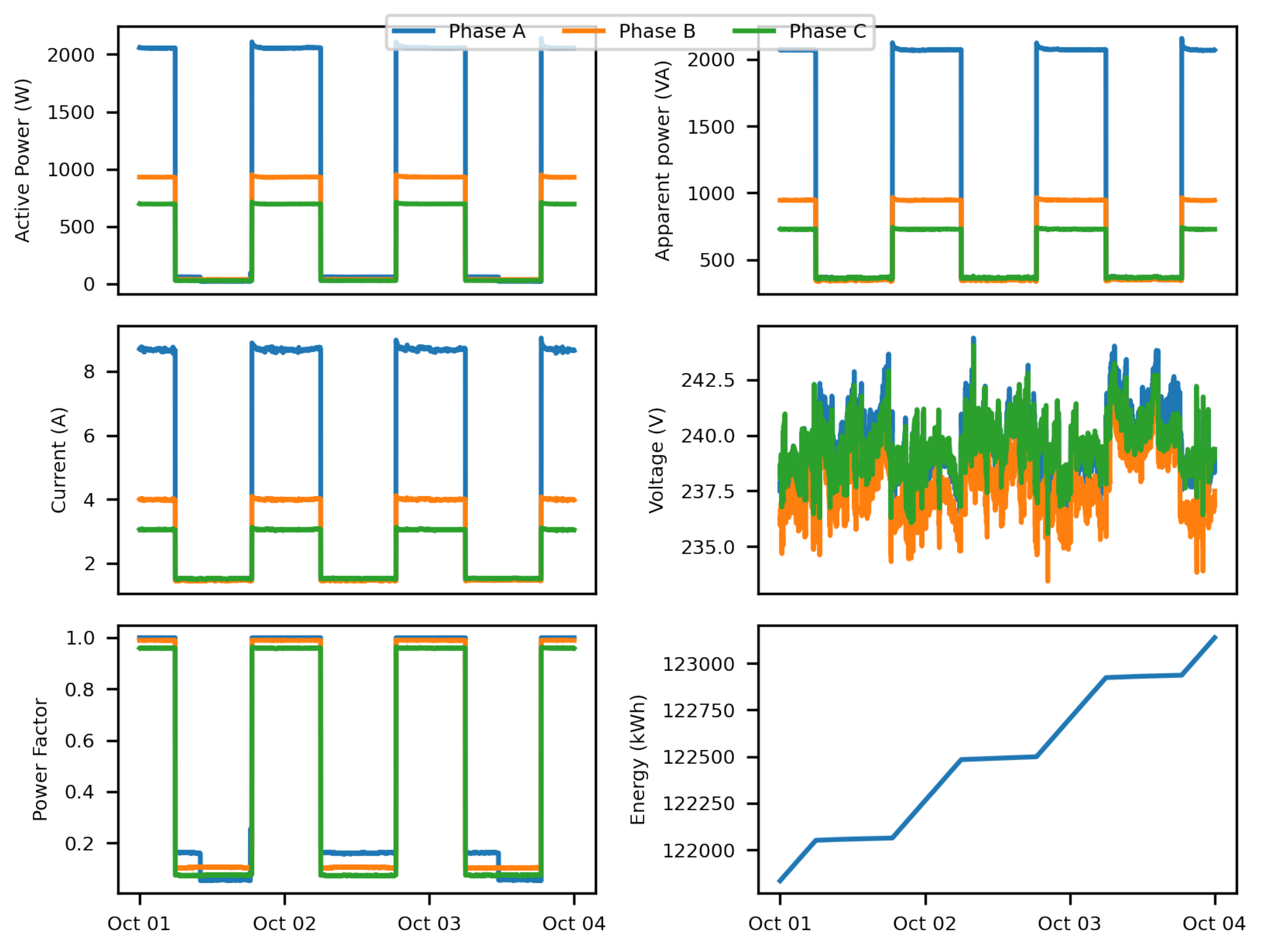
Lighting systems for roads and public places are based on the control of illumination switchboards, which include a lighting control cabinet used to distribute energy, control the moment of switching on and off the lighting, and protect the components from short circuits and overloads. Lamps are grouped into circuits connected to these cabinets. Because the cabinet power supply comprises three phases, each cabinet has three circuits, as shown in Figure 1. A certain number of lamps are connected to each circuit, depending on the street, road, or park configuration. The optimal solution an even distribution of the lamps between circuits, which is often impossible. As a result, dozens of lamps are often connected to a single circuit.

Verification of the anomaly detection algorithms in the present work is based on data from a smart lighting system installed in 2020 in the Polish city of Słupsk. The system comprises more than 4200 smart wirelessly managed LED lamps based on ZigBee technology. The lighting control system is equipped with 80 three-phase energy meters installed in street cabinets. Data from the meters are read at 60 s intervals and are transferred to a central database. Each record contains the following data:

• Meter ID;
• Date/time;
• Total energy;
• Phase voltage (VA, VB, and VC);
• Current (IA, IB, and IC);
• Active power (PA, PB, and PC);
• Apparent power (SA, SB, and SC);
• Power factor (PFA, PFB, and PFC).

Between June 2020 and November 2021, 48 million records were recorded in the database. Figure 2 shows an example of records for one of the meters (the horizontal axes show dates, and the vertical axes show measurement volumes).

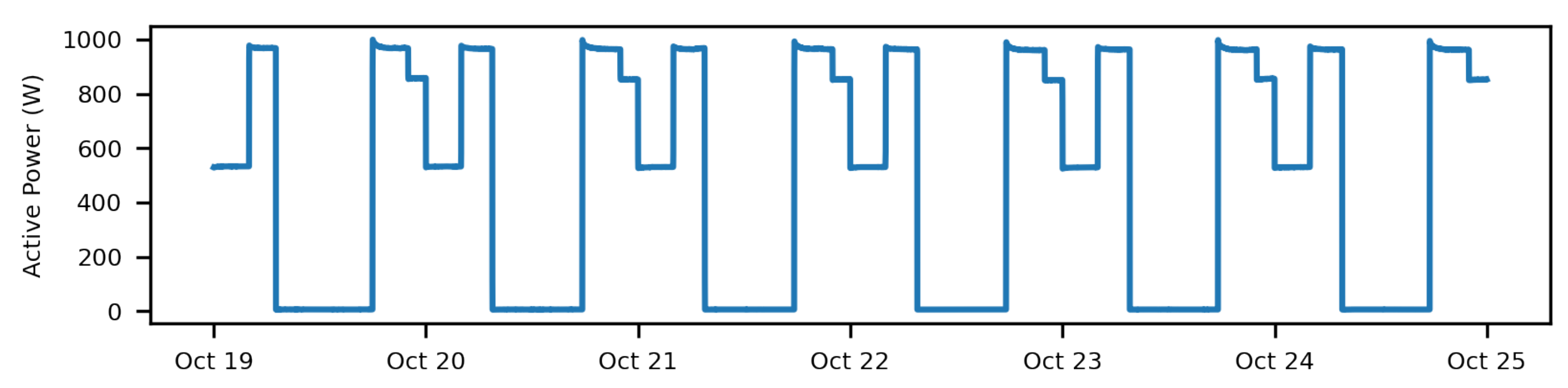
For this work, active power records were used. An example chart of the active power of one of the phases for lamps without reduction, that is, switched on at dusk and switched off at dawn, is shown in Figure 3. The database also includes measurements for lamps for to which lighting level reduction was applied. Figure 4 shows the active power graph for the following reduction schedule:

• Twilight—switch on lamps 100%;
• 22:00—reduction to 70%;
• 00:00—reduction to 40%;
• 04:00—turn off reduction, return to 100%;
• Dawn—shutdown.

Figure 3. Graph of the active power of one phase for lamps without reduction.

Figure 3. Graph of the active power of one phase for lamps without reduction.

Figure 4. Graph of the active power of one phase for lamps with reduction.

Figure 4. Graph of the active power of one phase for lamps with reduction.

Several to dozens of lamps are connected to the circuits assigned to each phase. In the installation described here, the average number of lamps per circuit is 20, and more than 90% of the circuits have fewer than 50 lamps. Lamps connected to a circuit can have different powers; in this installation, the power ranges from 52 W to 143 W. On average, lamps with a total power of 1200 W are connected to a circuit. For such a power rating, only 52 W lamps result in a 4.3% reduction in active power reading, which is above the resolution of energy meters. In this installation, meters were installed that implement active energy measurement in class 0.5 S according to IEC/EN 62053-22.

3. Types of Anomalies

Data from energy meters installed in residential buildings represent stochastic processes. The moments when appliances are switched on are not determined, although there are some regularities. Energy production by photovoltaic panels is also random. In the case of a road lighting system, the deterministic behavior of energy consumers should prevail; the lamps should switch on and off at predictable moments in time. The number of energy consumers (lamps) and their power ratings are generally fixed and defined. Instantaneous power consumption is also influenced by dynamic factors, such as ambient temperature, the moment of dawn and dusk in the case of astronomical clock control, the state of cloudiness in the case of twilight switch control, reductions in lighting intensity for luminaires operating based on schedules, and other events occurring in adaptive systems. As a result, the recorded data are also random.

Undesirable phenomena that should be detected as anomalies include the switching off of one or more lamps during the night, switching on of one or more lamps during the day, incorrect timing of switching lamps on or off, and incorrect power reduction in the system. A highly undesirable phenomenon is energy theft, which is the connection of an unauthorized energy consumer to the circuit supplying lamps. Other anomalies can also occur, such as misreading of data from meters and errors in the data recording system; however, we do not deal with these anomalies in this article. There is a direct relationship between the occurrence of anomalies and instantaneous power consumption. Examples of anomalies recorded in the real system are shown in Figure 5. Charts A, B, C, and D show anomalies related to control without reduction, and charts E and F show anomalies of control with reduction:

• A—switching on of lamps during the day;
• B—no switching on of lamps at night;
• C—some of the lamps are not working, resulting in a decrease in the power consumed;
• D—switching on of a group of lamps during the day or energy theft;
• E—disabling the reduction schedule;
• F—some of the lamps are not working, resulting in a decrease in the power consumed.

Figure 5. Examples of anomalies in energy consumption by the lighting system. Subfigures show examples of anomalies: (A) switching lamps on during the day; (B) no switching lamps on at night; (C) some of the lamps are not working; (D) switching a group of lamps on during the day; (E) disabling the reduction schedule; (F) some of the lamps are not working.

Figure 5. Examples of anomalies in energy consumption by the lighting system. Subfigures show examples of anomalies: (A) switching lamps on during the day; (B) no switching lamps on at night; (C) some of the lamps are not working; (D) switching a group of lamps on during the day; (E) disabling the reduction schedule; (F) some of the lamps are not working.

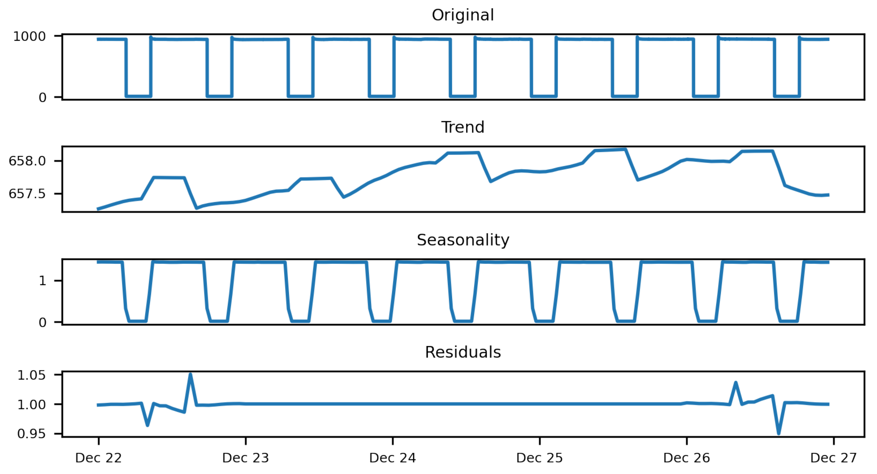
4. Time Series Analysis

Measurements of active power read from energy meters are made with a fixed period and are recorded with a time stamp, so they have the character of a time series. For the basic way of controlling road lighting without reduction, the waveform has the character of a unipolar rectangular wave with a period of 24 h and a variable duty cycle because the length of day and night changes during the year. The duty cycle is proportional to the length of the night (or day), which means that the average value of the waveform has a periodic character with a period of 1 year. Because the length of night is related to a location expressed in geographic coordinates, changes in the average value vary for each location. Figure 6 shows a graph of the power consumption duty cycle for the city of Gdańsk; the beginning and end of illumination are calculated according to sunsets and sunrises, i.e., the moments when the sun disc passes below the horizon. Figure 6 also shows a graph of the duty cycle according to civil twilights and dawns, when the center of the sun’s disc is 6 degrees below the horizon.

An algorithm described by NOAA’s Earth System Research Laboratory [22] based on a method defined in [23] was used for the calculations.

The active power time series is a univariate time series. Our goal is to use systematically recorded values to predict future values, that is, forecasting a univariate time series.

Because the time series of active power is a periodic signal, it is necessary to determine the components, i.e., trend, noise, and periodic. Then, using the decomposition method based on moving averages and an additive model (seasonal decomposition using moving averages), we obtain the result shown in Figure 7.

The decomposition result differs in terms of trend between seasons (Figure 8) because depending on the season, the nighttime—and therefore the length of light—lengthens or shortens.

With a measurement period of 1 min, the size of the time series period is 1440 samples. Unfortunately, the available ARIMA modeling tools do not allow for definition of such a period. Furthermore, the maximum length of the period is limited by computing power and memory requirements. Therefore, for the creation of the time series model, we decided to downsample the stream by calculating the average of the input period as 15 min, which resulted in a seasonal order period of 96. However, such a period also proved to be taxing on resources, so the stream was downsampled to a period of 1 h and a seasonal order with a period of 24. Figure 9 shows the decomposition for a series with a period of 60 min.

5. Experimental Conditions

The calculations used actual data from the energy meter registration database described above, from which sample sets of active power measurements were selected and divided into two groups. The first group contains measurements for such periods during which no anomalies occurred. These data come from three different meters for different seasons and for each phase, resulting in 9 sets labeled ZP₁, ZP₂, …, ZP₉. These sets have varying values of power measurement amplitudes, as they measure different circuits. The second group of sets contains measurements for time segments during which anomalies occurred, as shown in Figure 5. These sets were labeled ZP_A, ZP_B, …, ZP_F. The data in the sets were subjected to a data cleaning operation (data cleaning), which involves supplementing the sample string with missing records. Records were missing because they were recorded in real time, and any interruption in the operation of the device resulting, for example, from a reboot, results in periodic missing records.

All algorithms were implemented in Python version 3.10.5. The following libraries were used: pandas 1.3.5, NumPy 1.21.5, statsmodels 0.13.1, scikit-learn 1.0.2, TensorFlow 2.9.1, and Keras 2.9.0. The calculations were carried out on a computer with an Intel^® Core™ i7-7700HQ 2.8 GHz processor and 16 GB of RAM. A comparison of calculation times was performed on the Raspberry Pi hardware platform, Compute Module 4 model, with a quad-core ARM-8 Cortex-A72 (64-bit) 1.5 GHz processor and 4 GB of RAM.

6. SARIMA-Based Anomaly Detection Algorithm

The ARIM (autoregressive integrating moving average) model was used to model the time series. Assuming the periodic nature of the series, a periodic version was used, i.e., SARIMA (seasonal autoregressive integrated moving average). The following parameters define the SARIMA model:

• (p) autoregressive parameter;
• (d) the row of differentiation;
• (q) the moving average parameter;
• (P) autoregressive parameter for the period;
• (D) the order of differentiation for the period;
• (Q) the moving average parameter for the period;
• (m) seasonality period,

The following notation will be used hereafter (p,d,q) (P,D,Q) (m).

In our case, the parameter m = 24 is determined, and the other parameters must be selected. Traditional methods of setting model parameters are based on analysis of autocorrelation functions and partial autocorrelation of seasonality and trends [24]. Because the algorithm under development should be self-learning, an automatic parameter selection algorithm is used to determine the model parameters. An example algorithm for automatic parameter selection is the stepwise algorithm proposed in the [25]. This algorithm is widely used and has many implementations, including in R and Python. However, it uses the Akaike information criterion (AIC) parameter minimization criterion, which leads to a preference for models with less complexity at the expense of forecasting accuracy.

Another reason for using automatic parameter selection is changing data characteristics over time. Such change is caused, among other things, by a change in the length of night/day over a year, the number of lamps installed, or lamp types or by a change in the reduction schedule. These changes make the model parameters selected at the beginning of the observation obsolete, requiring reselection. This is referred to as concept drift [26]. This phenomenon also occurs in short-term load forecasting (STLF) in residential and non-residential buildings [27]. The authors of [27] point out that traditional ARIMA models, which are commonly used for STLF, do not have an incremental learning mechanism of forgetting outdated data and adapting to the latest measurements. Traditional methods only learn the parameters of a given ARIMA model once, using a fixed training set, and then apply the model to all future measurements. The authors proposed an incremental algorithm that periodically rebuilds the predictive model using the sliding window concept. A similar mechanism is implemented in the anomaly detection algorithm under development, except that the goal of the algorithm changes. In the OLIN algorithm, the goal is to determine the current energy consumption profile, whereas in the proposed solution, the goal is to detect anomalies. The second significant difference is a change in the way the model is validated.

Several methods are used to validate and test the time series mapping model; the most commonly used is MAPE (mean absolute percentage error), as specified in Equation (1):

$$MAPE=\frac{1}{n}{\displaystyle \sum }_{t=1}^n|\frac{y_t-y_t^P}{y_t}|\ast 100\%$$

(1)

The disadvantage of this measure is that it takes undefined values when the actual data are zero and takes extreme values when the actual data are very close to zero, which is the case with data from a lighting system.

This disadvantage is avoided by the MAE (mean absolute error) measure, for which the mean absolute error is defined by Equation (2):

$$MAE=\frac{1}{n}{\displaystyle \sum }_{t=1}^n\left|y_t-y_t^P\right|$$

(2)

This measure predicts the extent of deviation from the actual, on average, over the forecast period. The primary measure of the error between the forecast variable and the forecast is the absolute error, which is denoted as AE_t (absolute error; Equation (3)):

$$A{E}_t=|y_t-y_t^P|$$

(3)

For the anomaly detection problem, the maximum absolute error (MaAE) measure is also important for the resulting set of errors (Equation (4)):

$$MaAE=max{\left\{A{E}_t\right\}}_{t=0}^{N-1}$$

(4)

In order to ensure that comparisons can be made for waveforms with different amplitudes, we introduce a measure of normalized MaAE_norm proportional to the peak-to-peak value (Equation (5)):

$$MaA{E}_{norm}=100\%\ast \frac{MaAE}{Y_{max}-Y_{min}}$$

(5)

A grid search algorithm was used to search for model parameters (Algorithm 1). As input, the algorithm requires a training set (Y_tr) a validation set (Y_val) and a set of sets of acceptable values for SARIMA parameters: {p₁…p_p}, {d₁…d_d}, {q₁…q_q}, {P₁…P_P}, {D₁…D_D}, {Q₁…Q_Q}. From the set of parameter sets, a set of parameter vectors is created (p_m, d_m, q_m, P_m, D_m, Q_m). For each parameter set vector, a SARIMA model is created based on samples from the training set. Based on the model, a forecast “Out-of-sample” of length equal to the size of the validation set is calculated. Based on the forecast and the samples from the validation set, the MAE error is calculated and added to the list, along with the parameter vector. After the list is created, the parameter vector for which the MAE value is the smallest is selected.

For each set of samples, the algorithm can choose different model parameters. The selection of the number of samples for the training and validation sets is essential for the performance of the anomaly detection algorithm. A larger number of samples increases the accuracy of the models and the system response time to potential anomalies. For the training set, the minimum number of samples is defined, as in [28]. The proposed algorithm assumes two days or 48 samples. The size of the forecast should not exceed the seasonality period.

The anomaly detection algorithm works cyclically according to the rhythm of incoming data, i.e., readings from the smart meter. For each step, the absolute error (AE) is determined, which is used to decide whether to detect an anomaly.

In the first phase, samples are completed to form the training and validation set, which are used to produce the initial model using the grid search algorithm. Then, the algorithm performs the following operations in a loop: creating and training the SARIMA model, calculating the forecast based on the developed model, and determining the AE forecast error based on the actual measurement, which is used to decide whether to detect an anomaly. Then, the measurement window is moved by one sample, and new training and validation sets are determined, as shown in Figure 10. Based on these sets, the occurrence of concept drift (Algorithm 2) is verified. If the condition is met, the grid search algorithm is executed again. Algorithm 3 shows how to determine the AE set for the simulation.

The following inputs were used for the calculation: number of samples in the training set, N_tr = 48; validation set, N_val = 23; threshold for the need to search for new model parameters, D_Th = 1.1. The following sets of SARIMA parameter values were used to search for model parameters: p = {0, 1, 2}, d = {0, 1}, q = {0, 1, 2}, P = {0, 1}, D = {0, 1}, Q = {0, 1, 2}, resulting in 216 combinations.

Algorithm 1: Grid search parameters of the SARIMA model.
	Input:
	- Training set—Ytr
	- Validating set—Yval,
	- Parameters sets—{p1…pp}, {d1…dd}, {q1…qq}, {P1…PP}, {D…D1D}, {Q1…Q Q}
	Output:
	- MAE for model
	- parameters of model (p,d,q,P,D,Q)
1:	Generate cartesian product for parameter sets:
	M = {p1…pp} x {d1…dd} x {q1…qq} x {P1…PP} x {D…D1D} x {Q1…QQ}
2:	for each (pm, dm, qm, Pm,Dm,Qm) in M:
3:	create model: model = ARIMA (Ytr, (pm, dm, qm), (Pm, Dm, Qm), 24)
4:	fit the parameters of the model: model_fit = model.fit()
5:	make out-of-sample forecast: Yp = model_fit.forecast(len(Yval))
6:	calculate MAE: MAEm = MAE(Yval, Yp)
7:	add (MAEm, (pm, dm, qm, Pm, Dm, Qm)) to list {ML}
8:	return MAEx, (px, dx, qx, Px, Dx, Qx) for min(MAE) in {ML}

Algorithm 2: Concept drift detection.
	Input:
	- Training set—Ytr
	- Validating set—Yval,
	- Parameters of SARIMA model (pi, di, qi, Pi, Di, Qi)
	- Current model MAE—MAEi
	- Concept drift threshold—DTh
	Output:
	- new MAEo for model
	- new parameters of SARIMA model (po, do, qo, Po, Do, Qo)
1:	Create model: model = ARIMA (Ytr, (po, do, qo), (Po, Do, Qo), 24)
2:	Fit the parameters of the model: model_fit = model.fit()
3:	Make forecast: Yp = model_fit.forecast(len(Yval))
4:	Calculate MAE: MAEm = MAE(Yval, Yp)
5:	If MAEm/MAEi > DTh then
6:	Find parameters and MAE (Algorithm 1): MAEo, (po, do, qo, Po, Do, Qo) = GridSearch(Ytr, Yval)
7:	Else
8:	MAEo = MAEi
9:	(po, do, qo, Po, Do, Qo) = (pi, di, qi, Pi, Di, Qi)
10:	return MAEo, (po, do, qo, Po, Do, Qo)

Algorithm 3: Calculate absolute errors using SARIMA.
	Input:
	- Number of test steps—Ns
	- Number of training samples—Ntr
	- Number of validating samples—Nval
	- Set of samples of length = Ntr + Nval + Ns
	Output:
	- Calculated absolute errors {AE1, AE2, …, AENs}
1:	Calculate t0 = tstart, t1 = tstart + Ntr, t2 = t1 + Nval, t3 = t2 + 1
2:	Prepare training set Ytr [t0; t1], validating set Yval [t1; t2], actual value yt3
3:	Find initial parameters and MAE (Algorithm 1):
	MAEc, (pc, dc, qc, Pc, Dc, Qc) = GridSearch(Ytr, Yval)
4:	for i = 1 to Ns
5:	Create model: model = ARIMA (Ytr, (pc, dc, qc), (Pc, Dc, Qc), 24)
6:	Fit the parameters of the model: model_fit = model.fit()
7:	Make forecast: yp = model_fit.forecast(1)
8:	Calculate absolute error: AEi = |yp − yt3|
9:	Add AEi to list {AE}
10:	Calculate new window: t0 = t0 + 1, t1 = t1 + 1, t = t22 + 1, t3 = t3 + 1
11:	Prepare training set Ytr [t0; t1], validating set Yval [t1; t2], actual value yt3
12:	Check concept drift: MAEc, (pc, dc, qc, Pc, Dc, Qc) = ConceptDriftCheck(Ytr, Yval, (pc, dc, qc, Pc, Dc, Qc), MAEc, DTh)
13:	return {AE}

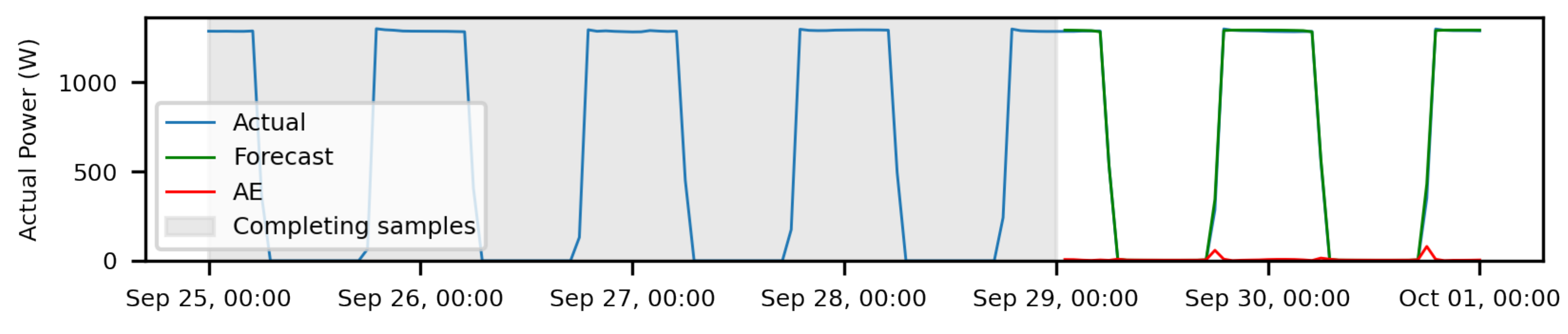
The simulation result for a set of ZP₁ measurements, i.e., records without anomalies, is shown in Figure 11. The gray box indicates the sample collection period. This period is 71 h because 48 h of training samples and 23 validation samples are needed. Only after this time does detection begin (white box). The label “Forecast” denotes the calculated forecast, and “AE” is the forecast absolute error.

The simulation was then repeated for all sets of ZP₁ …, ZP₉, calculating MAE and MaAE meters. Because the sets have different amplitudes of active power, the normalized value of MaAE_norm was also calculated; the results are included in

Table 1. Simulation results with the SARIMA algorithm for ZP sets₁ …, ZP₉.

Dataset	ZP1	ZP2	ZP3	ZP4	ZP5	ZP6	ZP7	ZP8	ZP9
MAE	8.51	8.75	4.72	3.25	2.89	2.18	2.29	4.53	2.10
MaAE	60.27	68.33	42.35	52.60	27.75	34.89	24.34	34.93	20.97
MaAEnorm	4%	5%	5%	5%	5%	5%	1%	2%	1%

, showing that for these sets, the maximum normalized value of MaAE_norm is equal to 5%, which may be the threshold for deviation from the typical waveform, i.e., anomaly.

Then, simulations were performed for sets with anomalies ZP_A, ZP_B, …, ZP_F. The simulation result is shown in Figure 12.

Table 2. Simulation results with the SARIMA algorithm for datasets ZP_A, …, ZP_F.

Dataset	ZPA	ZPB	ZPC	ZPD	ZPE	ZPF
MAE	30.89	221.99	119.97	101.49	19.30	48.03
MaAE	813.76	1499.33	342.00	532.44	189.79	159.56
MaAEnorm	99%	100%	40%	79%	43%	27%

contains the calculated values of MAE, MaAE, and MaAE_norm for the sets ZP_A, ZP_B, …, ZP_F. The computed data show that the lowest value of MaAE_norm is equal to 27%. Thus, selecting the error detection threshold in the <5%, 27%> range makes it possible to detect anomalies effectively.

The choice of thresholds makes it possible to determine the sensitivity of the algorithm and is related to the specific implementation of the algorithm. Figure 13 shows a simulation of the detection algorithm for 10% and 30% thresholds.

7. LSTM-Based Anomaly Detection Algorithm

The latest data modeling methods are based on deep machine learning techniques (deep learning) [29,30,31,32,33] using multilayer neural networks. For sequential data analysis, such as time series, recurrent neural networks (RNNs) are used to identify data structure and patterns. RNNs are trained by backpropagation through time (BPTT). However, for longer sequences, there is a problem of vanishing first inputs, also known as the vanishing gradient problem. A model called long short-term memory (LSTM) was developed to solve this problem [34,35]. LSTM networks consist of specific cells connected by layers equipped with memory and three nonlinear gates:

• Input, which decides how the input updates the memory state;
• Forgetting, which determines how values from the previous state update the memory state; and
• Output, which decides what to output based on input data and memory status.

The LSTM cell acts as a mini state machine that uses an internal memory cell to hold state values for an extended period, and the gates have weights that are calculated during the training procedure.

For the time series of active power measurements to become an input stream for machine learning, it is necessary to organize the data in such a way that a supervised learning mode can be used. Input data (X) and output data (Y) are fed to the network simultaneously so that the algorithm can learn to make predictions and minimize the differences between the expected and learned values. Therefore, it is necessary to transform the time series from a one-dimensional sequence to a two-dimensional matrix, one dimension of which represents the input data (features) and the other of which represents the output data (labels). For a sequence of measurements (t₀, t₁, …, t, t_N−1N), the values read from t₀, t₁, …, t_N−1 are features, and the value of t_N is a label.

As previously mentioned, the time series of active power measurements are characterized by a strong periodicity related to the daily rhythm, so it is natural for the constructed network to be able to predict the next active power value based on the previous day’s data. However, the 24 most recent time intervals are needed to predict the value in the next time interval, assuming a sampling period of 60 min.

When configuring an LSTM network, the number of hidden network layers is specified, as well as the size of the data vector transmitted by each layer. In addition, the network’s learning set size should be determined. Because in the case of an online algorithm, we are dealing with a constant influx of new samples, there is a kind of arbitrariness in choosing the size of the learning set. On the one hand, the larger the set, the greater the probability of obtaining a matched model. Moreover, a larger set means a longer startup delay for the detection algorithm and a more significant computational effort. In order to compare the LST-based anomaly detection algorithm with the SARIMA-based algorithm, it would be desirable to use the same period (3 × 24 h); however, this is not possible because the network is trained with a vector that is created based on 24 measurements. To obtained Ntr learning vectors, N_tr + N_F + N_L measurements are required, where N_F is the number of features, and N_L is the number of labels. In our case, for a learning set of 48 vectors, 73 samples are needed. Similarly, 49 samples are needed to obtain a test set of 24 vectors. In order to reduce the total set size, N_F recent samples from the learning set are used to produce the test vectors. The total number of samples for both sets in this connection is N_tr + N_F + N_L + N_val + N_F + N_L samples (in our case, 98 measurements).

Because there are no explicit methodologies for selecting the LSTM network architecture, a grid search algorithm analogous to that used in the SARIMA-based method was used to determine the optimal parameters. As input, the algorithm requires a training set (Y_tr), a validation set (Y_val), a set of sets of permissible values for the number of hidden network layers {l₁ …, l_l}, and the size of the vector transmitted by each layer {o₁ …, o_o}. From the set of parameter sets, a set of parameter vectors is created (l_m, o_m). A model is created for each parameter set vector with the appropriate number of layers and vector size. The model is trained with a fixed number of iterations (epochs) equal to 100 with samples from the learning set. From the model, a forecast for the test set is calculated; based on this forecast and samples from the test set, the MAE error is calculated, which, along with the parameter vector, is added to the list. After the list is created, the parameter vector for which the MAE value is the lowest is selected. The results of Algorithm 4 for the sets ZP₁, ZP₂, …, ZP₉ are shown in

Table 3. Simulation results of grid search algorithm parameters of the LSTM network.

Dataset	ZP1	ZP2	ZP3	ZP4	ZP5	ZP6	ZP7	ZP8	ZP9
Layers	5	5	5	5	4	5	5	1	5
Output space	1	1	1	1	1	1	1	7	1
Minimum MAE	3.87	6.58	3.24	4.27	3.63	3.07	6.57	10.86	5.88
Maximum MAE	32.44	33.54	21.49	33.86	19.83	24.01	27.11	31.11	24.45
Mean MAE	13.58	15.40	9.28	11.93	8.61	8.45	12.71	18.44	11.44

.

Algorithm 4: Grid search parameters of LSTM network.
	Input:
	- Number of training samples—Ntr
	- Number of validating samples—Nval
	- Set of samples Ntr + Nval
	- Parameters sets—{l1…ll}, {o1…oo}
	Output:
	- MAE for model
	- parameters of the model (layers, output space dimension)
1:	Split samples set to Training set—Ytr and Validating set—Yval
2:	Generate cartesian product for parameter sets: M = {l1…ll} x {o1…oo}
3:	for each (lm, om) in M:
4:	create model: LSTM(layers = lm, output_space = om)
5:	train model: model.fit(Ytr)
6:	make prediction: Yp = model. predict(Yval)
7:	calculate MAE: MAEm = MAE(Yval, Yp)
8:	add (MAEm, (lm, om)) to list {ML}
9:	return MAEx, (lx, ox) for min(MAE) in {ML}

The above algorithm adopts a fixed number of epochs, which is determined by observing the course of the loss function during cross validation. Part of the learning set is designed to carry out periodic validation during learning to control the learning process. The purpose of the control is to achieve the desired error rate and prevent overfitting. Figure 14 shows the plot of the loss function defined as the MSE (mean squared error) for the training and validation sets. The graph plots the functions for all tested sets (ZP₁, ZP₂, …, ZP₉). As can be seen, the loss function stabilizes quickly, and even with 200 iterations, there is no overfitting effect.

The following sets were assumed: network layers, l = {1, 2, 3, 4, 5}; output space, o = {1, 2, 3, …, 10}. The table contains the determined network configuration, the corresponding MAE value (minimum), and the maximum and average MAE values that occurred when testing all configurations.

Deep learning also suffers from concept drift [35,36,37,38,39,40], so a mechanism is needed to detect such a situation. Therefore, in the designed algorithm, a control mechanism is used by calculating the MAE value for the training set and checking at each step whether the error increases above the assumed threshold.

The anomaly detection algorithm using the LSTM model works analogously to the SARIMA-based algorithm (Algorithm 5). The operation starts with the collection of samples, forming a training and validation set, based on which the network configuration is determined using the grid search algorithm. Then, the model is created and trained with the combined training and validation sets. The algorithm then performs the following operations in a loop: calculating the forecast based on the developed model and determining the AE forecast error based on the actual measurement, is used to decide whether to detect an anomaly. Then, the measurement window is moved by one sample, a new training set is determined, it is verified that the calculated MAE for the forecast based on this set does not exceed the assumed threshold. If this condition is met, the grid search algorithm is executed again, and new network parameters are determined.

Algorithm 5: Calculate absolute errors using LSTM.
	Input:
	- Number of test steps—Ns
	- Number of training samples—Ntr
	- Set of samples of length = Ntr + Ns
	- Concept drift threshold—DTh
	Output:
	- Calculated absolute errors {AE1, AE2, …, AENs}
1:	Calculate t0 = tstart, t1 = tstart + Ntr, t2 = t1 − 24, t = t32 + Ns, t4 = t1 + 1
2:	Split samples set to Training set Ytr [t0; t1] and Testing set Ys [t2; t3]
3:	Find network configuration (Algorithm 4): (lc, oc) = GridSearch(Ytr)
4:	Create model: LSTM(layers = lc, output_space = oc)
5:	Train model: model.fit(Ytr)
6:	Make prediction on training set: Yp = model.predict(Ytr)
7:	Calculate MAE: MAEm = MAE(Ytr, Yp)
8:	for i = 1 to Ns
9:	Create model: model = ARIMA(Ytr, (pc, dc, qc), (Pc, Dc, Qc), 24)
10:	Make prediction: yp = model.predict(Yval [i])
11:	Calculate absolute error: AEi = |yp − yt4|
12:	Add AEito list {AE}
13:	Calculate new window: t0 = t0 + 1, t1 = t1 + 1, t = t22 + 1, t3 = t3 + 1, t = t44 + 1
14:	Prepare training set Ytr [t0; t1]
15:	Make prediction: Yp = model.predict(Ytr)
16:	Calculate MAEi = MAE(Ytr, Yp)
17:	If MAEi/MAEm > DTh then
18:	Find network configuration (Algorithm 4): (lc, oc) = GridSearch(Ytr)
19:	Create model: LSTM(layers = lc, output_space = oc)
20:	Train model: model.fit(Ytr)
21:	Make prediction: Yp = model. predict(Ytr)
22:	Calculate MAEm = MAE(Ytr, Yp)
23:	Else
24:	MAEm = MAEi
25:	return {AE}

Simulation according to the defined algorithm was performed for all datasets (ZP₁ …, ZP₉) calculating meters’ MAE, MaAE, and MaAE_norm. The sample collection period is longer than the SARIMA algorithm (98 h). The simulation result for the dataset ZP₁ measurement is shown in Figure 15, and the calculated meters are included in

Table 4. Simulation results with the LSTM algorithm for datasets ZP₁ …, ZP₉.

Dataset	ZP1	ZP2	ZP3	ZP4	ZP5	ZP6	ZP7	ZP8	ZP9
MAE	7.44	11.47	7.79	6.71	3.90	4.59	5.92	8.02	5.38
MaAE	80.46	101.61	71.16	59.36	37.98	41.34	65.94	69.21	59.79
MaAEnorm	6%	7%	8%	6%	6%	6%	4%	4%	4%

.

Then, simulations were performed for sets with anomalies (ZP_A, ZP_B, …, ZP_F). The simulation result is shown in Figure 16.

Table 5. Simulation results with the LSTM algorithm for datasets ZP_A, …, ZP_F.

Dataset	ZPA	ZPB	ZPC	ZPD	ZPE	ZPF
MAE	49.04	515.68	189.91	75.52	28.53	43.17
MaAE	812.69	1476.98	338.83	482.01	186.01	152.79
MaAEnorm	99%	99%	40%	72%	42%	26%

contains the calculated values of MAE, MaAE, and MaAE_norm for the sets ZP_A, ZP_B, …, ZP_F. Among the calculated data, the lowest value of MaAE_norm is equal to 26%. Thus, it is possible to assume an error detection threshold in the range of <8%, 26%>. The interval is therefore narrower than that of the SARIMA algorithm.

Figure 17 shows the simulation of the detection algorithm for 10% and 30% thresholds.

8. Comparison of Results

Both of the proposed algorithms have been shown to be effective in detecting anomalies in the analyzed datasets. However, the algorithms differ in terms of time series mapping. The comparison result of the basic measures is shown in

Table 6. Comparison of algorithm simulation results for datasets ZP₁ …, ZP₉.

Dataset	ZP1	ZP2	ZP3	ZP4	ZP5	ZP6	ZP7	ZP8	ZP9	MEAN
SARIMA MAE	8.51	8.75	4.72	3.25	2.89	2.18	2.29	4.53	2.10	4.36
SARIMA MaAE	60.27	68.33	42.35	52.60	27.75	34.89	24.34	34.93	20.97	40.71
LSTM MAE	7.44	11.47	7.79	6.71	3.90	4.59	5.92	8.02	5.38	6.80
LSTM MaAE	80.46	101.61	71.16	59.36	37.98	41.34	65.94	69.21	59.79	65.20
MAE (LSTM − SARIMA)	−1.07	2.72	3.08	3.46	1.00	2.41	3.63	3.48	3.28	2.44
MaAE (LSTM − SARIMA)	20.19	33.28	28.81	6.76	10.23	6.45	41.60	34.28	38.82	24.49
MAE (LSTM − SARIMA) %	−14%	24%	39%	52%	26%	52%	61%	43%	61%	38%
MaAE(LSTM − SARIMA) %	25%	33%	40%	11%	27%	16%	63%	50%	65%	37%

for the sets ZP₁ …, ZP₉, and

Table 7. Comparison of algorithm simulation results for datasets ZP_A, …, ZP_F.

Dataset	ZPA	ZPB	ZPC	ZPD	ZPE	ZPF	MEAN
SARIMA MAE	30.89	221.99	119.97	101.49	19.30	48.03	90.28
SARIMA MaAE	813.76	1499.33	342.00	532.44	189.79	159.56	589.48
LSTM MAE	49.04	515.68	189.91	75.52	28.53	43.17	150.31
LSTM MaAE	812.69	1476.98	338.83	482.01	186.01	152.79	574.89
MAE (LSTM − SARIMA)	18.14	293.69	69.94	−25.97	9.23	−4.86	60.03
MaAE(LSTM − SARIMA)	−1.07	−22.35	−3.17	−50.43	−3.78	−6.77	−14.59
MAE (LSTM − SARIMA) %	37%	57%	37%	−34%	32%	−11%	20%
MaAE(LSTM − SARIMA) %	0%	−2%	−1%	−10%	−2%	−4%	−3%

shows comparison results for the sets ZP_A, …, ZP_F. The presented data show that the algorithm based on the SARIMA model has a higher accuracy in mapping the time series of active power measurements; the average MaAE is 38% lower for this model than for the LSTM for waveforms without anomalies. With respect to the average MaAE, the difference is similar, at 37%. For waveforms with anomalies, the differences are smaller and depend on the type of waveform.

A Raspberry Pi miniature computer was used to compare algorithm execution times because under real conditions, this computing performance is representative when applying the edge computing concept. The comparison of times is included in

Table 8. Comparison of algorithm stage times.

	SARIMA	LSTM
Sample collection time (h)	71	98
Search time for model parameters (s)	113	2400
Prediction calculation time per sample (s)	41	2

.

The comparison shows that the SARIMA-based algorithm requires less time to reach anomaly detection readiness. Although the LSTM-based algorithm has a 20 times shorter forecast calculation time, the hyperparameter search time is more than 20 times longer. In addition, both algorithms can run in real time using a hardware platform comparable to the Raspberry Pi, as the analysis time for a single measurement is less than the sampling period of 60 min.

The shorter algorithm startup time and greater accuracy in mapping the time series of active power measurements ultimately indicate the superiority of the SARIMA-based algorithm.

9. Conclusions

The practical feasibility of using power measurements from energy meters to detect anomalies in a lighting system was demonstrated in this paper. The possibility of creating a self-learning algorithm that does not require feature extraction and an online-type algorithm that detects anomalies in a limited time was also shown. The used sampling period of 60 min is justified for effective monitoring of a lighting system because for the investigated type of installation, the demanded response time to a failure is many hours or even days.

The developed algorithms offer the possibility of industrial implementation, which is practical because the requirements for the equipment used in this study are reasonably low. To implement the function, relatively inexpensive hardware is required, i.e., a typical smart energy meter. Furthermore, the lighting control system used for experiments allows for the transmission of measurements from energy meters to the computing cloud, where detection algorithms and local processing according to the edge computing paradigm can be implemented.

An additional advantage of monitoring lighting systems is that monitoring can be applied to various light sources, namely traditional, discharge, and modern LED types.