Abstract
This research aims to predict knock occurrences by deep learning using in-cylinder pressure history from experiments and to elucidate the period in pressure history that is most important for knock prediction. Supervised deep learning was conducted using in-cylinder pressure history as an input and the presence or absence of knock in each cycle as a label. The learning process was conducted with and without cost-sensitive approaches to examine the influence of an imbalance in the numbers of knock and non-knock cycles. Without the cost-sensitive approach, the prediction accuracy exceeded 90% and both the precision and the recall were about 70%. In addition, the trade-off between precision and recall could be controlled by adjusting the weights of knock and non-knock cycles in the cost-sensitive approach. Meanwhile, it was found that including the pressure history of the previous cycle did not influence the classification accuracy, suggesting little relationship between the combustion behavior of the previous cycle and knock occurrence in the following cycle. Moreover, learning the pressure history up to 10° CA before a knock improved the classification accuracy, whereas learning it within 10° CA before a knock did not noticeably affect the accuracy. Finally, deep learning was conducted using data, including multiple operating conditions. The present study revealed that deep learning can effectively predict knock occurrences using in-cylinder pressure history.
1. Introduction
In recent years, improving thermal efficiency and reducing emissions have been major goals in spark-ignition (SI) engine development. Among the many methods studied to reach these goals, increasing the compression ratio and advancing the spark timing are effective. However, these measures tend to induce knocking [1].
Knocking is caused by auto-ignition of the unburned fuel-air mixture that has become hot and pressurized between the flame front and the cylinder walls. This leads to engine failures, such as piston crown melting, cylinder head erosion, piston ring breakage, and decreased engine efficiency [1,2]. Thus, knocking needs to be suppressed.
Currently, a vibration sensor attached to the engine is used to detect knocking. Upon detection of knocking, it is automatically suppressed by retarding the spark timing [3]. However, the location of knocking in the cylinder varies from cycle to cycle [2]. Moreover, even in a steady-state condition, knocking occurs in some cycles but not in others [4]. Therefore, the current knock-suppression measure may excessively retard the spark timing in cycles in which knocking is not likely to occur, deteriorating the thermal efficiency of SI engines. Consequently, a technology to preliminarily predict the occurrence of knocking for each cycle is required, whereby the knock-suppression measures are applied to cycles only in which knocking is likely to occur. Such a method allows the prevention of knocking and achieves high thermal efficiency by increasing the compression ratio and advancing the spark timing. In summary, the cycle-by-cycle prediction of knocking can be an effective strategy to improve the engine thermal efficiency.
Since knocking is a complex phenomenon, detecting and predicting knocking cycle-by-cycle is a difficult task [2]. However, by utilizing the ability of deep learning to automatically extract features contained in the data, the need to determine indices and thresholds of knock prediction or detection for each engine and operating condition can be eliminated. Deep learning is a method of learning data features through multiple levels of abstraction using a multi layered computational model [5] called a neural network. In recent years, the accuracy of deep learning has improved significantly enough to make it applicable to various fields. A well-known example of deep learning in the automotive research field is object detection around a vehicle in autonomous driving [6].
Deep learning and neural networks have also been applied to internal combustion engine research. Many research groups have predicted performance and emissions by artificial neural networks (ANNs) using data obtained from each operating condition [7,8,9,10,11,12]. In particular, many studies have included mixture ratios of fuel components as inputs for ANN [13,14,15,16,17,18]. Regarding performance and emissions, one model has predicted BMEP and combustion phase, while another has predicted volumetric efficiency [19,20]. In addition to performance and emission predictions, spray characteristics, heat release, and COVIMEP (an indicator of cycle-to-cycle variation) are also being predicted [21,22,23]. Other studies have examined replacing engine controllers, predicting EGR rates, and detecting pre-ignition [24,25,26].
In recent years, some studies have been conducted to predict or detect knocking using deep learning. As for the studies of knock prediction based on operating conditions, Shin et al. [27] constructed a deep neural network (DNN) model to predict knock occurrence, performance, and emissions using parameters of operating conditions. Zhou et al. [28] used sensor data to predict super-knock occurrence from parameters of operating conditions. Since super-knock is a very rare phenomenon, that study mentioned an imbalance in the amount of data between normal operating conditions and operating conditions in which super-knock occurs.
Meanwhile, as stated by Cho et al. [29], a cycle-by-cycle analysis of in-cylinder pressure history is required to detect or predict knocking. They used in-cylinder pressure history from knock cycles to predict the timing of knock occurrence and were able to detect knocking at intensities too low for conventional detection methods. On the other hand, Kefalas et al. [30] performed continuous wavelet transform on the in-cylinder pressure history of each cycle and detected knocking by using a convolutional neural network (CNN). They showed that if data from completely different engines were used for the training and test data, the detection accuracy would be lowered, or detection would not be possible. Another study by Ofner et al. [31] used a 1-D CNN to detect knocking by using in-cylinder pressure history as input. Because it took less than 1 ms to classify each cycle, this method can be used for real-time control. They also showed the possibility of dealing with data of unknown operating conditions.
However, to the authors’ knowledge, there are no studies that use in-cylinder pressure history to predict knocking on a cycle-by-cycle basis using deep learning. Therefore, in this study, we performed deep learning to predict knock occurrence using cyclic in-cylinder pressure history and to explore the features that lead to knock occurrence in the data used for the learning process. We then aimed to establish a new, low-cost knock prediction method that is fast enough to be useful for real-time control.
2. Method
2.1. Dataset
Supervised deep learning requires a data set of input data and labels for each input. In this study, the input was the in-cylinder pressure history for each cycle and the label was the knock occurrence in that cycle.
Table 1 shows the specifications of the engine used to collect the data. To ensure reliable ignition and promote flame propagation in lean fuel conditions, this engine had an enhanced ignition system and a customized intake adapter to enhance the in-cylinder tumble flow [32]. In addition, thermal efficiency was improved by a high compression ratio, and the S/V ratio was reduced by a long stroke to reduce cooling losses. An electric supercharger was also used.

Table 1.
Engine specifications.
In this study, in-cylinder pressure history for two cycles was input as a set. As a result, the range of one pressure history set was extended to −1080° ATDC–360° ATDC. In addition, although 400 cycles were measured for each operating condition, the first cycle did not have a previous cycle, so the subsequent data set consisted of 399 cycles per condition. The time resolution of the data was 1° CA.
In this study, the widely used maximum amplitude of in-cylinder pressure oscillation [2] was used for knock detection. The knock detection procedure is illustrated in Figure 1. A pressure wave generated by knocking has peaks at specific frequencies, and the resonance frequency of each vibration mode can be obtained by the formula proposed by Draper [33]. The in-cylinder temperature of the operating condition used in Section 3.1, Section 3.2, Section 3.3 was estimated using an in-house code, which analyzes the in-cylinder pressure under the assumption of an ideal gas and quasi-static process with a uniform mixture. The calculated average temperature at 8° ATDC, which is the timing just before knocking occurred, was 1408 K. Substituting the temperature into the formula, the resonance frequencies of the (1,0), (2,0), (0,1), (3,0), and (1,1) modes were 5.68, 9.42, 11.8, 13.0, and 16.5 Hz, respectively. Therefore, in this study, a bandpass filter of 4–20 kHz was applied to the experimentally obtained in-cylinder pressure. The maximum value of the one-sided amplitude was defined as the knock intensity, and the cycle in which the intensity exceeded 50 kPa was defined as the knock cycle. As for the cut-off frequencies of the bandpass filter, Zhen et al. [2] state that the lower limit is usually 4 kHz, and the higher limit is well above the frequency of the in-cylinder oscillations. In addition, the cut-off frequencies and threshold used in this study were the same as the study using the same engine [34].
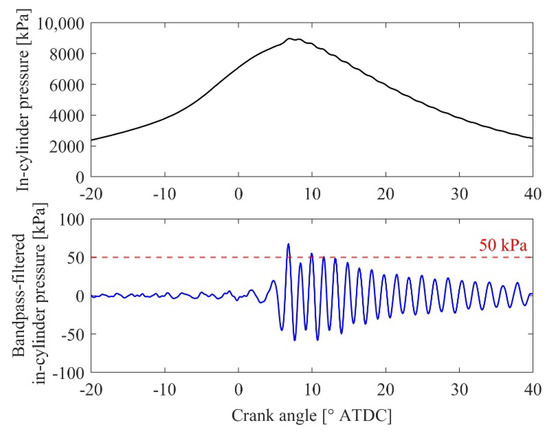
Figure 1.
Knock detection procedure. Top: Measured in-cylinder pressure history. Bottom: Knock intensity is the maximum value of the one-sided amplitude of in-cylinder pressure after the bandpass filter is applied. The cycle in which the value exceeded 50 kPa was defined as the knock cycle.
The knock intensity for each cycle for the operating conditions used in Section 3.1 and Section 3.2 is shown in Figure 2. Out of 399 cycles, 63 were determined to be knocking.
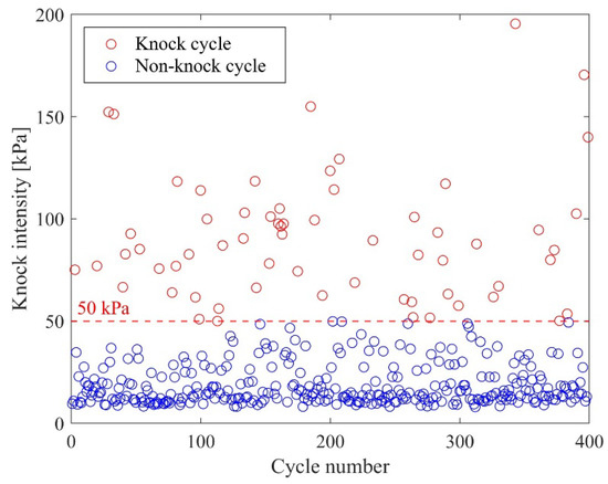
Figure 2.
Knock intensity for each cycle.
2.2. Deep Learning Model
In this study, in-cylinder pressure was input to DNN. The number of neurons in the input layer was set to be equal to the number of input values [5]. For example, the deep learning model in Section 3.1 used the in-cylinder pressure of 360° ATDC–0° ATDC with the time resolution of 1° CA as the input, so the number of neurons in the input layer was 361. The number of neurons in the output layer in the classification problem should be equal to the number of classes to classify [5]. In this study, the number of neurons in the output layer was two, corresponding to knocking and non-knocking.
The DNN structure was tailored to the longest time range of the input data (720° CA), and the number of neurons in the hidden layers was reduced by the same ratio, from 721 to 2. The number of hidden layers was set to 3, and then the numbers of neurons in those hidden layers were 540, 360, and 180, respectively. This number of layers was obtained by trying several numbers of layers.
The activation function for the hidden layer was ReLU (Rectified Linear Unit) [35]. A softmax function, which is commonly used in the classification problem, was used as the activation function of the output layer [35]. Cross-entropy error was used as the loss function [35].
An Adam optimizer [36] was used with an initial learning rate of 0.01, and this rate was then reduced to one-tenth every 10 epochs. The rate was reduced because, if the learning rate is too large, the parameters may diverge, or the learning process may not proceed once a certain level of accuracy is achieved. If it is too small, on the other hand, the learning process may take too long.
Batch normalization was applied after the weighted sums in the hidden layers were computed [37]. In this normalization process, the input data for each mini-batch are standardized, and then a scale factor and a shift factor are applied. Batch normalization is expected to speed up deep learning by increasing the learning rate while suppressing overfitting [37].
Dropout [38] is a method to suppress overfitting by randomly deleting neurons during training. In the test process, the signal is transmitted to all neurons, but the output is multiplied by the ratio erased during training [38]. In this study, we applied dropout to each hidden layer at a rate of 50%.
In this study, the batch size was 32 and the epoch was 50.
All deep learning procedures were performed using MATLAB R2021a and Deep Learning Toolbox.
2.3. Evaluation
As shown in Figure 3, the classification results by the neural network are divided into four categories, depending on the combination of predicted class and actual class. Each element of the matrix contains the number of applicable data.
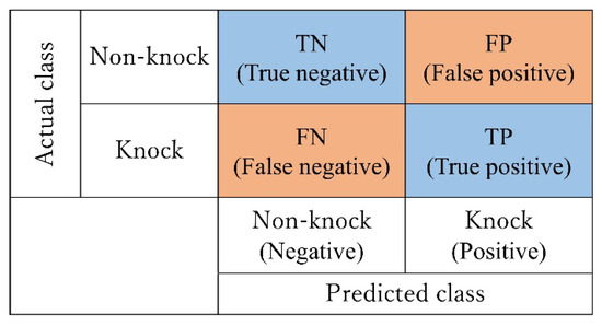
Figure 3.
Confusion matrix.
In this study, four statistical indices are used. Accuracy [35] indicates the ratio of correct data to all data classified by the network and can be obtained by using each element of the confusion matrix as shown in Formula (1).
There are two types of accuracy: training accuracy, which is obtained using training data to check the progress during training, and test accuracy, which is obtained using test data to evaluate the neural network.
Precision and recall [35] are obtained by Formula (2) and Formula (3), respectively. In this study, precision indicates the percentage of cycles in which knocking occurred among the cycles in which knocking was predicted, and recall indicates the percentage of cycles in which knocking was predicted among those in which knocking occurred. In general, there is a trade-off between precision and recall.
The F-measure, which is the harmonic mean of precision and recall, is also used for evaluation [35]. The F-measure is represented by Formula (4).
2.4. Imbalanced Learning
In classification problems, the algorithm will be biased by the imbalance in the amount of data in each class (in this study, two classes: one with and one without knocking), and such a case is called imbalanced learning [39]. In other words, the algorithm is more likely to predict a majority class, and recall may become very small. Engines are not operated under conditions where knocking occurs in about half of the total cycles, and in the data used in this study, about 15% of the cycles are knocking. So, in this study, there is a risk of predicting a knock cycle as non-knock. To tackle this problem, two methods are used: undersampling and cost-sensitive learning.
- Undersampling
Undersampling corrects the imbalance in the amount of data between classes by randomly extracting the data from the majority group and adjusting the number to the minority group. This method often leads to the removal of important data contained in the majority group. Moreover, overfitting is likely to occur since the total number of data is reduced.
- Cost-sensitive learning
Cost-sensitive learning changes weights when a knock cycle is mistaken for a non-knock one and vice-versa. In this study, a bigger weight was assigned to the minority class so that the neural network emphasized the minority class (knock) and prevented the neural network from easily predicting the majority class (non-knock).
Cost-sensitive learning is performed by changing the loss function. The weighted cross-entropy error [40] provided in Equation (5) is expressed by adding a weight term to the cross-entropy error
where m is the mini-batch size, wk is the weight for the class k, tlk indicates that the l-th data in the mini-batch belongs to the k-th class, and ylk is the output of the k-th neuron for the l-th data.
In general, the reciprocal of the number of data included in each class is used as the ratio of weights between classes [41]. In the data used in this study, the ratio wnon-knock:wknock is about 0.15:0.85. In addition to the reciprocal, several weights (0.2:0.8, 0.3:0.7, 0.4:0.6) were used to connect the result up to the point where there is no imbalanced learning (wnon-knock:wknock = 0.5:0.5).
2.5. k-Fold Cross-Validation
In this study, k-fold cross-validation is performed to ensure model robustness [27]. In this method, all the data are divided into k folds. The first fold is used for the test and the remaining k−1 folds are used for training, Then, the second fold is used for the test and the rest are used for training. This sequence is repeated k times, and the average value of the k results is used for the evaluation.
In a general hold-out method, all data are used for either training or testing, but in k-fold cross-validation, essentially all data are used once for testing, making the result less susceptible to data bias.
In one k-fold cross-validation method, called stratified k-fold cross-validation, data imbalance remains the same among folds when the data are divided into k folds. Stratified k-fold cross-validation is used for classification problems in which the amounts of data are imbalanced between classes.
This study used stratified 5-fold cross-validation, which gave the best results when tested at k = 5 and k = 10, with stratified and nonstratified cross-validation.
3. Results and Discussion
3.1. Reference Model
For the operating condition used for deep learning in Section 3.1, Section 3.2, Section 3.3, S5H [42], a surrogate fuel of premium gasoline was used. The other parameters were as follows: excess air ratio of 2.1, spark timing of −31.5° ATDC, and IMEP of 0.8 MPa. Using these data, knock occurrence was predicted using in-cylinder pressure history from −360° ATDC, the timing at which each cycle starts, to the top dead center (0° ATDC) of that cycle. As mentioned above, there were three hidden layers, which respectively contained 540, 360, and 180 neurons. Stratified 5-fold cross-validation was used, and 316 and 79 cycles were assigned for training and testing, respectively. Since there were 63 knock cycles and 336 non-knock cycles, 12 knock cycles and 67 non-knock cycles were assigned to each fold. Thus, a total of 79 cycles were assigned to each fold.
The results are shown in Table 2. The average test accuracy was over 90%, and both precision and recall were 70% or higher. These results showed that the neural network can predict knock occurrence.
Table 2.
Prediction results using only data before knocking.
For imbalanced learning, undersampling and cost-sensitive learning were performed. The weights for cost-sensitive learning were 0.2:0.8, 0.3:0.7, and 0.4:0.6 as well as the reciprocal (≈0.15:0.85), which is the reciprocal of the number of data included in each class. In the following, we denote these weights as cost(0.2:0.8), cost(0.3:0.7), cost(0.4:0.6), and cost(reciprocal), respectively. The case where imbalanced learning is not performed is denoted as normal.
In undersampling, overfitting occurred and generalization ability could not be acquired. Figure 4 shows the loss of both the training data and the test data for normal and undersampling. Overfitting is considered to have occurred when the test loss is much larger than the training loss. The cause of overfitting was that the number of cycles assigned to the training data was small. In undersampling, only 96 cycles were used for the training data, whereas 316 cycles were used in non-undersampling cases.
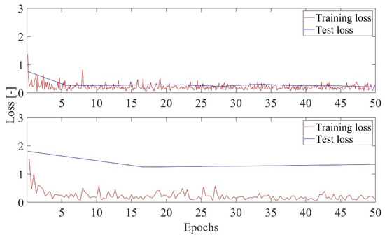
Figure 4.
Training loss and test loss in normal (top) and undersampling (bottom).
Figure 5 shows the relationship between precision and recall in normal and cost-sensitive learning. It can be confirmed that there is a trade-off between precision and recall. For example, in a cycle where a trained deep learning model predicts knocking, a countermeasure using the prediction can suppress knocking by the amount of recall and thus prevent damage to the engine. However, the same countermeasure is performed for normal cycles at the probability of 1 minus precision. So, it is important to balance the trade-off by changing the weights, considering the disadvantages of the countermeasure.
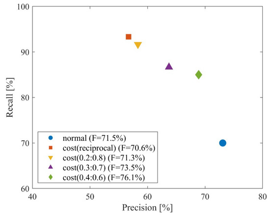
Figure 5.
Relationship between precision and recall.
The results of normal and cost-sensitive learning were evaluated in terms of the F-measure. Hereafter, cost(0.4:0.6) is used for the discussion since it showed the highest value.
3.2. Influence of the Start CA on Prediction
In this section, the starting point of the in-cylinder pressure used in the input data was changed to compare the deep learning results when the input data include the in-cylinder pressure of the previous cycle or when the data are shortened. The five starting points vary from −720° ATDC, which is the top dead center of the previous cycle, to −32° ATDC, which is close to the spark timing of the target cycle. The end point of the input data was set to 0° ATDC. As mentioned above, the cost-sensitive learning of cost(0.4:0.6) was used. The other parameters were the same as described above. Training accuracy, test accuracy, precision, and recall are shown in Figure 6. The evaluation indices were similar for all ranges, and prediction was possible even for the shortest range, −32° ATDC–0° ATDC.
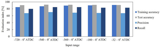
Figure 6.
Effects of changing the start CA on prediction.
The absence of any consistent trend in the values suggested that the in-cylinder pressure from −720° ATDC to −32° ATDC showed no characteristics that would lead to the prediction of knock occurrence. In this study, we assumed that the combustion conditions of the previous cycle would affect the knock occurrence in the next cycle and that the inclusion of the in-cylinder pressure history of the previous cycle in the input data would improve prediction performance. However, such results were not obtained. It was considered that, in knock occurrence, the initial stage of combustion has a more significant effect than the residual gas from the previous cycle due to internal EGR.
Here, we attempted to visualize the results of the knock occurrence prediction. In Figure 7, the in-cylinder pressure is color-coded according to the results of the prediction using −32° ATDC–0° ATDC.
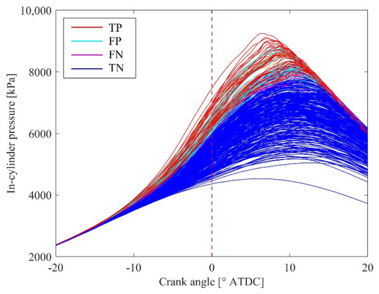
Figure 7.
In-cylinder pressure color-coded by predicted class and actual class based on the results of the prediction using −32° ATDC–0° ATDC.
Overall, the higher cycles are predicted as knocking, while the lower cycles are predicted as non-knocking. However, multiple cycles corresponding to TN and TP intersect near the boundary. This indicates that the in-cylinder pressure at 0° ATDC is not the only factor used to determine the threshold, but that the rate of increase in in-cylinder pressure, the timing at which the pressure begins to increase, and the relationship between them are also considered.
3.3. Influence of the End CA on Prediction
In this section, the end point of the in-cylinder pressure used in the input data was changed to verify the effect of the pressure range on the accuracy of knock occurrence prediction. The starting point of the input data was set to −32° ATDC, and the end points were set to −15, −10, −5, 0, and +5° ATDC. Cost-sensitive learning of cost(0.4:0.6) was used, and the other parameters are the same as described above. Judging from the pressure history of the operating condition used in this section, knocking occurs after 5° ATDC.
Figure 8 shows the training and test accuracy, precision, and recall. All indices increase from −32° ATDC–−15° ATDC to −32° ATDC–0° ATDC. These results indicate that the importance of in-cylinder pressure in predicting knock occurrence increases as the timing of knock occurrence approaches. On the other hand, the values are similar between −32° ATDC–0° ATDC and −32° ATDC–+5° ATDC, showing that in-cylinder pressure history closer to the timing of knock occurrence does not improve prediction accuracy. This is a very important result. For example, if a trained neural network provides real-time control and feedback to suppress knocking in an actual engine, the length of the data used for the prediction can be adjusted depending on both the accuracy and the time required for control.
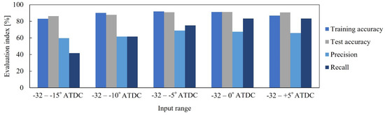
Figure 8.
Effects of changing the end CA on prediction.
3.4. Using Multiple Operating Conditions for Deep Learning
Since engines are used under multiple operating conditions, deep learning models need to adapt to those conditions. In addition, the number of training data can be increased by using multiple operating conditions.
In this section, the operating condition used so far is referred to as ➀, and three additional operating conditions, ➁, ➂, and ➃, are added to the data set. The experimental conditions are shown in Table 3. For conditions ➁, ➂, and ➃, the equivalence ratio is 1.0; the fuels are CP50, CP50, and NM5; the spark timings are −6.6, +0.4, and −1.5° ATDC; and IMEP are 0.8, 1.0, and 0.8 MPa, respectively. CP50 is S5H with 50% by volume of cyclopentane, which has a knock-suppressing effect. NM5 is S5H with 5% by volume of nitromethane, which has a knock-inducing effect.
Table 3.
Experimental conditions.
If the equivalence ratio and ignition timing change, the timing at which the in-cylinder pressure begins to rise and the degree of increase will also change, resulting in a different waveform of the in-cylinder pressure. So, the timing at which the in-cylinder pressure reaches its maximum, i.e., the timing of knock occurrence, also changes accordingly. Therefore, it is inappropriate to use a fixed crank angle as the input range for prediction using multiple operating conditions; instead, it is necessary to determine the input range for each operating condition. In this study, the following pre-processing procedure (shown in Figure 9) was conducted to unify data usage.
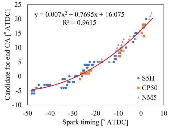
Figure 9.
Relationship between spark timing and the candidate for the end CA, and the approximation formula.
- For operating conditions ➀–➃ and operating conditions that used the same engine and fuel but are not used for deep learning, determine the timing (hereafter called the candidate for the end CA) that separates the spark timing and the timing of maximum in-cylinder pressure at 3:1.(This 3:1 ratio is necessary because the 0° ATDC, which splits about 3:1 between −31.5° ATDC and around 10° ATDC when knocking occurs, was important in operating condition ➀ used in Section 3.1, Section 3.2, Section 3.3)
- For each operating condition, plot the candidate for the end CA against the spark timing and approximate it with a quadratic polynomial.
- Let f be an approximation formula and use end CA = f (spark timing) to determine the end CA to be used for knock prediction for each operating condition.
Cost-sensitive learning of cost(0.4:0.6) was performed using the data of 360° CA before the end CA determined by the procedure for each operating condition. By stratified 5-fold cross-validation, 1272 and 318 cycles were used for training and test, respectively.
The results are shown in Table 4. The test accuracy is in the upper 80% range, and the recall is about 50%. Although the performance of the model deteriorated when multiple operating conditions were used, it can be said that the prediction was successful.
Table 4.
Results of deep learning using multiple operating conditions.
Here, again, the results of the knock occurrence prediction were visualized. Figure 10 shows the in-cylinder pressure color-coded according to the prediction results. At first glance, the neural network appears to be able to distinguish between the four operating conditions. However, in the three operating conditions in the lower right, some cycles appear to have been incorrectly predicted as a result of interference among the operating conditions. Therefore, the diminished accuracy may be attributable to the interference caused by similar in-cylinder pressure values among the operating conditions. Additionally, the accuracy might have been influenced by the differences in the number of knock cycles, which varied from 51 to 73 among the four conditions.
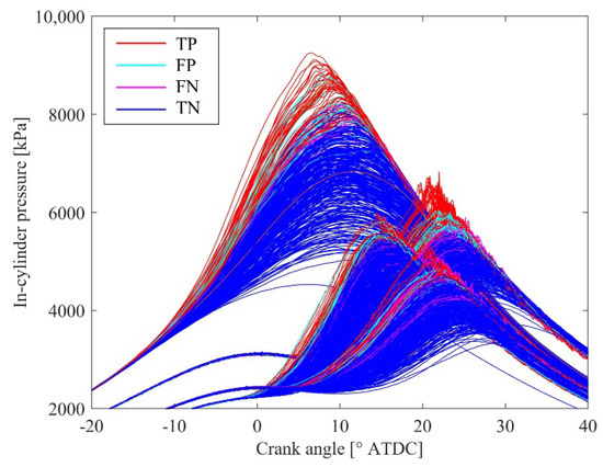
Figure 10.
In-cylinder pressure color-coded by predicted class and actual class based on the results of the prediction using multiple operating conditions.
In this study, deep learning was performed using a three-layer neural network under only one or four sets of operating conditions due to the constraints of computational cost and the amount of data retained, but from the engineering perspective, there were several important findings. Deep learning can predict knocking with a high accuracy, and it is also possible to change the balance between precision and recall by changing the weights of cost-sensitive learning. In addition, it was found that the length of data used for the prediction can be adjusted according to both the accuracy and the time required for real-time control of knocking. However, when multiple operating conditions were used, knock occurrence was predicted less accurately than with a single operating condition. In the future, larger numbers of operating conditions can be assessed, and common data for each operating condition can be added to the cyclic data. Moreover, by using a neural network with deep layers and high expressive power that can remove interference among operating conditions, highly accurate prediction becomes possible through the use of large amounts of data, which is one of the advantages of deep learning. The present success of deep learning with a single operating condition is considered to be the first step toward this goal.
4. Conclusions
Knocking is a major hindrance to improving the thermal efficiency of SI engines. In this study, deep learning was performed by using cyclic in-cylinder pressure history measured in experiments to predict knock occurrence in each cycle. The features that led to knocking in the data used for the learning process were also examined. The findings of this study are shown in the following:
- Using only the in-cylinder pressure data before the onset of knocking, the prediction accuracy was 91.4%, and both precision and recall were over 70%. In addition, cost-sensitive learning was applied to tackle the imbalance in the amount of data between the knock cycle and the non-knock cycle. When we adjusted the weight, this approach was able to control the balance between precision and recall.
- Changing the start CA of the pressure history input to the neural network, including the pressure history of the previous cycle, did not influence the classification accuracy, and the early stage of combustion was found to greatly affect the knock occurrence.
- Changing the end CA of the pressure history input to the neural network, even if data up to the timing immediately before the knocking were not used, enabled the prediction of knock occurrence with the same accuracy as when data up to the timing immediately before the knock occurrence were used.
- When multiple operating conditions were used for deep learning, the prediction accuracy remained high, but the recall was decreased compared to the model using a single operating condition, as a result of interference among the conditions.
Author Contributions
Conceptualization, H.T., T.T. and T.Y.; methodology, H.T.; software, H.T.; validation, H.T., T.T. and T.Y.; formal analysis, H.T.; investigation, H.T.; resources, H.T.; data curation, H.T.; writing—original draft preparation, H.T.; writing—review and editing, H.T., T.T. and T.Y.; visualization, H.T.; supervision, T.Y.; project administration, H.T. and T.Y.; funding acquisition, T.Y. All authors have read and agreed to the published version of the manuscript.
Funding
This research received no external funding.
Data Availability Statement
Not applicable.
Acknowledgments
The authors are grateful to Hidetsugu Yamamoto, and Hiroyuki Komatsu for providing technical support.
Conflicts of Interest
The authors declare no conflict of interest.
References
- Wang, Z.; Liu, H.; Reitz, R.D. Knocking combustion in spark-ignition engines. Prog. Energy Combust. Sci. 2017, 61, 78–112. [Google Scholar] [CrossRef]
- Zhen, X.; Wang, Y.; Xu, S.; Zhu, Y.; Tao, C.; Xu, T.; Song, M. The engine knock analysis—An overview. Appl. Energy 2012, 92, 628–636. [Google Scholar] [CrossRef]
- Kiencke, U. Automotive Control Systems for Engine, Driveline, and Vehicle, 2nd ed.; Springer: Berlin/Heidelberg, Germany, 2005. [Google Scholar]
- Kalghatgi, G.; Algunaibet, I.; Morganti, K. On knock intensity and superknock in SI engines. SAE Int. J. Engines 2017, 10, 1051–1063. [Google Scholar] [CrossRef]
- LeCun, Y.; Bengio, Y.; Hinton, G. Deep learning. Nature 2015, 521, 436–444. [Google Scholar] [CrossRef] [PubMed]
- Ma, Y.; Wang, Z.; Yang, H.; Yang, L. Artificial intelligence applications in the development of autonomous vehicles: A survey. IEEE/CAA J. Autom. Sin. 2020, 7, 315–329. [Google Scholar] [CrossRef]
- Taghavifar, H.; Taghavifar, H.; Mardani, A.; Mohebbi, A.; Khalilarya, S.; Jafarmadar, S. Appraisal of artificial neural networks to the emission analysis and prediction of CO2, soot, and NOx of n-heptane fueled engine. J. Clean. Prod. 2016, 112, 1729–1739. [Google Scholar] [CrossRef]
- Kapusuz, M.; Ozcan, H.; Yamin, J.A. Research of performance on a spark ignition engine fueled by alcohol-gasoline blends using artificial neural networks. Appl. Therm. Eng. 2015, 91, 525–534. [Google Scholar] [CrossRef]
- Chakraborty, A.; Roy, S.; Banerjee, R. An experimental based ANN approach in mapping performance-emission characteristics of a diesel engine operating in dual-fuel mode with LPG. J. Nat. Gas Sci. Eng. 2016, 28, 15–30. [Google Scholar] [CrossRef]
- Lotfan, S.; Ghiasi, R.A.; Fallah, M.; Sadeghi, M.H. ANN-based modeling and reducing dual-fuel engine’s challenging emissions by multi-objective evolutionary algorithm NSGA-II. Appl. Energy 2016, 175, 91–99. [Google Scholar] [CrossRef]
- Domínguez-Sáez, A.; Rattá, G.A.; Barrios, C.C. Prediction of exhaust emission in transient conditions of a diesel engine fueled with animal fat using artificial neural network and symbolic regression. Energy 2018, 149, 675–683. [Google Scholar] [CrossRef]
- Fang, X.H.; Papaioannou, N.; Leach, F.; Davy, M.H. On the application of artificial neural networks for the prediction of NOx emissions from a high-speed direct injection diesel engine. Int. J. Engine Res. 2021, 22, 1808–1824. [Google Scholar] [CrossRef]
- Sayin, C.; Ertunc, H.M.; Hosoz, M.; Kilicaslan, I.; Canakci, M. Performance and exhaust emissions of a gasoline engine using artificial neural network. Appl. Therm. Eng. 2007, 27, 46–54. [Google Scholar] [CrossRef]
- Ghobadian, B.; Rahimi, H.; Nikbakht, A.M.; Najafi, G.; Yusaf, T.F. Diesel engine performance and exhaust emission analysis using waste cooking biodiesel fuel with an artificial neural network. Renew. Energy 2009, 34, 976–982. [Google Scholar] [CrossRef]
- Yusaf, T.F.; Buttsworth, D.R.; Saleh, K.H.; Yousif, B.F. CNG-diesel engine performance and exhaust emission analysis with the aid of artificial neural network. Appl. Energy 2010, 87, 1661–1669. [Google Scholar] [CrossRef]
- Javed, S.; Satyanarayana Murthy, Y.V.V.; Baig, R.U.; Prasada Rao, D. Development of ANN model for prediction of performance and emission characteristics of hydrogen dual fueled diesel engine with Jatropha Methyl Ester biodiesel blends. J. Nat. Gas Sci. Eng. 2015, 26, 549–557. [Google Scholar] [CrossRef]
- Channapattana, S.V.; Pawar, A.A.; Kamble, P.G. Optimisation of operating parameters of DI-CI engine fueled with second generation Bio-fuel and development of ANN based prediction model. Appl. Energy 2017, 187, 84–95. [Google Scholar] [CrossRef]
- Mehra, R.K.; Duan, H.; Luo, S.; Rao, A.; Ma, F. Experimental and artificial neural network (ANN) study of hydrogen enriched compressed natural gas (HCNG) engine under various ignition timings and excess air ratios. Appl. Energy 2018, 228, 736–754. [Google Scholar] [CrossRef]
- Finesso, R.; Spessa, E.; Yang, Y.; Conte, G.; Merlino, G. Neural-network based approach for real-time control of BMEP and MFB50 in a euro 6 diesel engine. SAE Tech. Pap. 2017. [Google Scholar] [CrossRef]
- Luján, J.M.; Climent, H.; García-Cuevas, L.M.; Moratal, A. Volumetric efficiency modelling of internal combustion engines based on a novel adaptive learning algorithm of artificial neural networks. Appl. Therm. Eng. 2017, 123, 625–634. [Google Scholar] [CrossRef]
- Taghavifar, H.; Mardani, A.; Mohebbi, A.; Taghavifar, H. Investigating the effect of combustion properties on the accumulated heat release of di engines at rated EGR levels using the ANN approach. Fuel 2014, 137, 1–10. [Google Scholar] [CrossRef]
- Taghavifar, H.; Khalilarya, S.; Jafarmadar, S. Diesel engine spray characteristics prediction with hybridized artificial neural network optimized by genetic algorithm. Energy 2014, 71, 656–664. [Google Scholar] [CrossRef]
- Gürgen, S.; Ünver, B.; Altın, İ. Prediction of cyclic variability in a diesel engine fueled with n-butanol and diesel fuel blends using artificial neural network. Renew. Energy 2018, 117, 538–544. [Google Scholar] [CrossRef]
- Fujiwara, S.; Iwase, M.; Satoh, Y. Near Boundary Control of Automotive Engine using Machine Learning. In Proceedings of the International Conference on Advanced Mechatronic Systems (ICAMechS), Hanoi, Vietnam, 10–13 December 2020; pp. 69–73. [Google Scholar]
- Jung, D.; Hwang, I.; Jo, Y.; Jang, C.; Han, M.; Sunwoo, M.; Chang, J.H. In-cylinder pressure-based convolutional neural network for real-time estimation of low-pressure cooled exhaust gas recirculation in turbocharged gasoline direct injection engines. Int. J. Engine Res. 2021, 22, 815–826. [Google Scholar] [CrossRef]
- Kuzhagaliyeva, N.; Thabet, A.; Singh, E.; Ghanem, B.; Sarathy, S.M. Using deep neural networks to diagnose engine pre-ignition. Proc. Combust. Inst. 2021, 38, 5915–5922. [Google Scholar] [CrossRef]
- Shin, S.; Lee, S.; Kim, M.; Park, J.; Min, K. Deep learning procedure for knock, performance and emission prediction at steady-state condition of a gasoline engine. Proc. Inst. Mech. Eng. Part D J. Automob. Eng. 2020, 234, 3347–3361. [Google Scholar] [CrossRef]
- Zhou, Z.; Xiong, S.; Chen, Y.; Zhang, C.; Cao, Y. Deep learning approach for super-knock event prediction of petrol engine with sample imbalance. Fuel 2022, 311, 122509. [Google Scholar] [CrossRef]
- Cho, S.; Park, J.; Song, C.; Oh, S.; Lee, S.; Kim, M.; Min, K. Prediction modeling and analysis of knocking combustion using an improved 0D RGF model and supervised deep learning. Energies 2019, 12, 844. [Google Scholar] [CrossRef]
- Kefalas, A.; Ofner, A.B.; Pirker, G.; Posch, S.; Geiger, B.C.; Wimmer, A. Detection of knocking combustion using the continuous wavelet transformation and a convolutional neural network. Energies 2021, 14, 439. [Google Scholar] [CrossRef]
- Ofner, A.B.; Kefalas, A.; Posch, S.; Geiger, B.C. Knock detection in combustion engine time series using a theory-guided 1-D convolutional neural network approach. IEEE/ASME Trans. Mechatron. 2022, 27, 4101–4111. [Google Scholar] [CrossRef]
- Tsuboi, S.; Miyokawa, S.; Matsuda, M.; Yokomori, T.; Iida, N. Influence of spark discharge characteristics on ignition and combustion process and the lean operation limit in a spark ignition engine. Appl. Energy 2019, 250, 617–632. [Google Scholar] [CrossRef]
- Draper, C.S. Pressure waves accompanying detonation in the internal combustion engine. J. Aeronaut. Sci. 1938, 5, 219–226. [Google Scholar] [CrossRef]
- Nagasawa, T.; Okura, Y.; Yamada, R.; Sato, S.; Kosaka, H.; Yokomori, T.; Iida, N. Thermal efficiency improvement of super-lean burn spark ignition engine by stratified water insulation on piston top surface. Int. J. Engine Res. 2020, 22, 1421–1439. [Google Scholar] [CrossRef]
- Goodfellow, I.; Bengio, Y.; Courville, A. Deep Learning; The MIT Press: Cambridge, MA, USA, 2016. [Google Scholar]
- Kingma, D.P.; Ba, L.J. Adam: A Method for Stochastic Optimization. In Proceedings of the International Conference on Learning Representations (ICLR), San Diego, CA, USA, 7–9 May 2015; pp. 1–15. [Google Scholar]
- Ioffe, S.; Szegedy, C. Batch Normalization: Accelerating Deep Network Training by Reducing Internal Covariate Shift. In Proceedings of the 32nd International Conference on International Conference on Machine Learning, Lille, France, 6–11 July 2015; pp. 448–456. [Google Scholar]
- Srivastava, N.; Hinton, G.; Krizhevsky, A.; Sutskever, I.; Salakhutdinov, R. Dropout: A simple way to prevent neural networks from overfitting. J. Mach. Learn. Res. 2014, 15, 1929–1958. [Google Scholar]
- Krawczyk, B. Learning from imbalanced data: Open challenges and future directions. Prog. Artif. Intell. 2016, 5, 221–232. [Google Scholar] [CrossRef]
- Classification Output Layer—MATLAB Classification Layer. Available online: https://www.mathworks.com/help/deeplearning/ref/classificationlayer.html (accessed on 14 October 2022).
- Cui, Y.; Jia, M.; Lin, T.Y.; Song, Y.; Belongie, S. Class-Balanced Loss Based on Effective Number of Samples. In Proceedings of the 2019 IEEE/CVF Conference on Computer Vision and Pattern Recognition (CVPR), Long Beach, CA, USA, 15–20 June 2019; pp. 9260–9269. [Google Scholar]
- Miyoshi, A. Chemical kinetic analysis on the effect of the occurrence of cool flame on SI knock. Int. J. Automot. Eng. 2017, 8, 130–136. [Google Scholar] [CrossRef][Green Version]


Publisher’s Note: MDPI stays neutral with regard to jurisdictional claims in published maps and institutional affiliations. |
© 2022 by the authors. Licensee MDPI, Basel, Switzerland. This article is an open access article distributed under the terms and conditions of the Creative Commons Attribution (CC BY) license (https://creativecommons.org/licenses/by/4.0/).