Representation Learning for Detecting the Faults in a Wind Turbine Hydraulic Pitch System Using Deep Learning

Abstract

Wind turbine operators usually use data from a Supervisory Control and Data Acquisition system to monitor their conditions, but it is challenging to make decisions about maintenance based on hundreds of different parameters. Information is often hidden within measurements that operators are unaware of. Therefore, different feature extraction techniques are recommended. The pitch system is of particular importance, and operators are highly motivated to search for effective monitoring solutions. This study investigated different dimensionality reduction techniques for monitoring a hydraulic pitch system in wind turbines. These techniques include principal component analysis (PCA), kernel PCA and a deep autoencoder. Their effectiveness was evaluated based on the performance of a support vector machine classifier whose input space is the new extracted feature set. The developed methodology has been applied to data from a wind farm consisting of five 2.3 MW fixed-speed onshore wind turbines. The available dataset is composed of nine pitch events representing normal and faulty classes. The results indicate that the features extracted by the deep autoencoder are more informative than those extracted by PCA and kernel PCA. These features led to the achievement of a 95.5% F1-score, proving its superiority over the traditional usage of original features.

1. Introduction

Nowadays, wind farms are critical infrastructures for every country, especially with the power production market changing because of Russian gas restrictions. The power produced by wind farms is expected to balance the demand and keep the levelised cost of energy as low as possible. However, wind farm production depends on the wind conditions and the availability of wind turbines, meaning that they should be fault-free for when there are ideal conditions for power production. The latter is the only factor that can be controlled by humans; thus, the condition monitoring of wind turbines is crucial to ensure their availability. As a result, predictive maintenance can also lower the cost of the produced energy. According to the latest data from Danish wind farms [1,2], the operation and maintenance (O&M) costs of a wind turbine, regarding the market price, correspond to approximately 1.3–1.6 euro cents/kWh to ensure the profitability of the asset. The levelised cost of energy produced by an onshore wind turbine is assumed to be between 3.94 and 5.01 euro cents/kWh when under favourable wind conditions [3]. For this reason, operators are urged to lower these costs by utilising more sophisticated tools for scheduling their maintenance tasks. The Supervisory Control and Data Acquisition (SCADA) system is a key element in achieving these goals. Every wind turbine, regardless of the manufacturer, is equipped with a SCADA system whose task is to store the sensor measurements in a database at a specific time interval. Therefore, this system provides a cheap solution for monitoring the status of the components of a wind turbine, but more complex techniques are indispensable for taking full advantage of SCADA signals. Thus, it is not necessary to install more sensors and further increase the complexity. Typical time intervals include 10 s, 1 min or 10 min periods, during which a set of statistical measures, such as the average and standard deviation, are stored for each measured parameter.

The condition monitoring of wind turbines has been the subject of a notable number of studies in the literature [4,5,6,7]. Various forms of machine learning, including deep learning techniques, have been applied for monitoring, and they have been summarised in corresponding review papers [8,9]. However, modern statistical and artificial intelligence techniques can also provide efficient solutions to search for hidden information within SCADA data. When this hidden information is extracted, algorithms can work more efficiently, often with fewer parameters that are rich in information. These techniques constitute a field of machine learning/deep learning called manifold learning [10,11]. For instance, during the condition monitoring of wind turbines, these new extracted features can be fed to advanced machine learning/deep learning techniques to detect and predict faults. Furthermore, a feature extraction task leads to a set of more representative features that can unveil the differences between all possible fault types. Thus, the fault extraction task allows transferability, where the same developed model for extracting features can be used in other systems or fault types. Finally, automating the feature-engineering process is aligned with the current trend of end-to-end learning processes, proving its importance in the industry [12].

According to the literature, several researchers have used these techniques for wind turbine monitoring, that is, to reduce the dimensions of SCADA features and extract new, more informative ones. Their efforts have been focused mainly on using principal component analysis (PCA) before fault detection [13,14], PCA before fault detection in a distributed generation system [15] and PCA before blade fault detection [16]. In addition, autoencoders and their variations, which are based on nonlinear relationships, seem to be quite popular among researchers in wind turbine monitoring. More specifically, an autoencoder for dimensionality reduction has been applied before the diagnosis of blade icing [17] and, more generally, for wind turbine fault detection [18,19,20]. Additionally, advanced versions of autoencoders have been used, such as a deep joint variational autoencoder (JVAE) for gearbox monitoring [21], a moving-window-stacked multilevel denoising AE (MW-SMDAE) [22], sparse-dictionary-learning-based adversarial variational autoencoders (AVAE_SDL) [23] and a stacked denoising autoencoder [22] for wind turbine fault detection.

However, feature extraction has not been reported in the literature for the case of pitch system monitoring, which, according to several surveys [24,25,26], has the highest number of failures and one of the longest downtimes compared with the rest of the systems. The literature is limited only to the use of the original feature set using an adaptive neuro-fuzzy inference system (ANFIS) [27,28,29,30,31], support vector machine (SVM) for classification [32,33,34] and regression [35], and asymmetric SVM [36] and Gaussian processes [37,38]. The one exception is Wu et al. [18], who have suggested a multilevel denoising autoencoder to detect a pitch system fault but have done so without mentioning any additional information about the specific components of the pitch system. Therefore, it is indispensable to investigate dimensionality reduction—or, in other words, feature extraction techniques—in the case of hydraulic pitch system monitoring.

The purpose of the present study is to investigate feature extraction techniques for the fault detection of a wind turbine hydraulic pitch system. The studied techniques include PCA, kernel PCA (KPCA) and a deep autoencoder, representing linear and nonlinear transformations of the input space. All of these techniques transform the high-dimensional input space into lower dimensions. These extraction techniques are assessed in the context of SVM implementation. The novelty of the present study is that no other paper has investigated feature extraction and fault detection in a supervised manner for hydraulic pitch systems. Additionally, the current study highlights the dependence of each original monitoring feature on the new extracted ones by calculating the mutual information scores. This procedure is essential and clarifies the importance of this process. The available dataset contains several features related to the hydraulic pitch system, which are stored by SCADA in 10 min intervals. The dataset includes a set of nine pitch events of different types presenting healthy and faulty operations. Hence, the advantage of having a dataset full of diverse faults of pitch systems is very beneficial. Furthermore, among the three methods, the best performance has been demonstrated by the developed autoencoder.

The rest of the current paper is organised as follows: In Section 2, PCA, KPCA and the autoencoder for dimensionality reduction and feature extraction are described. In Section 3, the SVM theory for classification is demonstrated. Section 4 refers to the dataset and original SCADA features, while Section 5 presents the training and evaluation process of the developed model. The results of the present paper are included in Section 6, followed by conclusions in the last section.

2. Feature Extraction Methods

2.1. Principal Component Analysis (PCA)

PCA is a very popular technique used not only for dimensionality reduction but also for data compression, feature extraction, data visualisation and the data preprocessing task, focusing mainly on the standardisation of features [10,39]. PCA, which is alternatively known as the Karhunen–Loève transform, is a linear dimensionality reduction technique. From a group of correlated variables, it allows us to obtain a set of linearly uncorrelated vectors called principal components (PCs) or scores. The main concept behind PC transformation is to find the most informative projections that maximise variances [40]. The obtained PCs are mutually uncorrelated and ordered by descending explained variance. PCA is an unsupervised technique, meaning that it requires only the input, not the output, values.

PCA is based on orthogonal projections of the input space to another subspace called the principal subspace. Suppose that the input space is a collection of N points x_n = (x₁, x₂, …, x_N)^T in ${ℝ}^m$. Assuming a centred input space, the average of every feature should be equal to zero. This requirement should be fulfilled before implementing the PCA algorithm. The idea behind PCA is to find a linear and orthogonal projection of the high-dimensional input space m to a lower one (let it be p) that is sufficient to provide an adequate approximation of the original data. This dimensionality reduction must ensure the maintenance of most of the information that is included in the original data. Thus, a lower representation of x_n could be z_n ϵ ${ℝ}^p$, whose expression is given in Equation (1).

$$z_n=W^T{x}_n$$

(1)

where W is the pxp orthogonal matrix. After applying PCA, we have as many principal components as the number of original features. Z_n is also known as the latent vector, consisting of latent values that are not observed in the data [41]. The dimension of z_n is the same as x_n after applying PCA, but because the goal is to drastically reduce this dimension, a lower value, p, is selected according to the criteria mentioned below. W should be equal to matrix U, which contains p eigenvectors with the largest eigenvalues of the empirical covariance matrix, which is given in Equation (2). Therefore, the problem of linear dimensionality reduction is transformed into the problem of calculating the eigenvectors of covariance matrix D.

$$D=\frac{1}{N}{\displaystyle \sum }_{n=1}^N{x}_n{x}_n{}^T$$

(2)

If matrix U contains u_i eigenvectors, the eigenvalues, λ_i, must be found through Equation (3):

$${\lambda }_i·u_i=D·u_i, i=1,\dots , m$$

(3)

where λ_i is an eigenvalue of the empirical covariance matrix (D), and u_i is the corresponding eigenvector. After calculating the eigenvectors, PCs are calculated via Equation (4), such that the optimal solution of the reconstruction error is as if the orthogonal matrix is equal to the eigenvector matrix.

$$z_n\left(i\right)=u_i{}^T{x}_n, i=1, \dots , m$$

(4)

Dimensionality reduction is accomplished by selecting the first several PCs, $z_n\left(i\right)$, which are in descending order of variance or, in other words, in descending order of eigenvalues. PCA results in mutually uncorrelated principal components, whose number is selected based on different methods, which include setting an arbitrary threshold for the cumulative explained variance or looking at a scree plot, which is a plot of eigenvalues with respect to the number of principal components. Each eigenvalue gives the variance along its axis.

2.2. Kernel PCA

Often, linear models have limited effects in complex systems; thus, nonlinear ones are needed. Kernel PCA is a nonlinear generalisation of PCA that employs the kernel trick. Kernel PCA relies on an eigendecomposition of a full matrix of pairwise similarities in the feature space instead of the ambient space, which is executed when implementing PCA [41]. The basic concept of kernel PCA is to expand the features by nonlinear transformations into a high-dimensional feature space φ(x_n) ($\phi \in {ℝ}^L$) and then apply PCA in the new feature space. Thus, a linear PCA in φ(x_n) corresponds to a nonlinear PCA in the original data space x_n because x_n is replaced by φ(x_n).

Kernel PCA requires the calculation of eigenvalues but avoids working in the feature space φ(x_n). The eigenvalue problem is expressed in Equation (5):

$${\lambda }_i·v_i=S·v_i, i=1,\dots , L$$

(5)

where matrix S is the L × L sample of the covariance matrix of φ(x_n), which is given in Equation (6), λ_i is one of the nonzero eigenvalues of the sample covariance matrix (S) and v_i is the corresponding eigenvector. The expression shown in Equation (6) requires that the projected dataset is centred, meaning that it has a zero mean (${\displaystyle \sum }_n\phi \left(x_n\right)=0$).

$$S=\frac{1}{N}{\displaystyle \sum }_{n=1}^N\phi \left(x_n\right)\phi {\left(x_n\right)}^T$$

(6)

Combining Equations (5) and (6), vector v_i ends up being a linear combination of φ(x_n), whose coefficients are the a_i parameters in Equation (7):

$$v_i=\frac{1}{N}{\displaystyle \sum }_{n=1}^N{a}_{in}\phi \left(x_n\right)$$

(7)

Replacing v_i in Equation (5) with the expression given in Equation (7), Equation (8) is obtained by also introducing the expression $K\left(x_n,x_m\right)=\phi {\left(x_n\right)}^T\phi \left(x_m\right)$, which ends up as an equation that includes the kernel function K. Equation (8) can be further simplified into Equation (9), which gives the eigenvalues of the new problem after fulfilling the requirement of normalising the eigenvectors in the feature space.

$$\frac{1}{N}{\displaystyle \sum }_{n=1}^{N}K\left(x_l,x_n\right){\displaystyle \sum }_{l=1}^L{a}_{il}K\left(x_n,x_l\right)={\lambda }_i{\displaystyle \sum }_{n=1}^N{a}_{in}K\left(x_l,x_n\right)$$

(8)

$$K{a}_i={\lambda }_{i}N{a}_i, i=1,\dots , L$$

(9)

After formulating the new eigenvalue problem in the feature space, which is presented in Equation (9), the PCs for x_n are given by Equation (10), which is essentially PCA implementation in the feature space.

$$t_i\left(x\right)=\phi {\left(x_n\right)}^T{v}_i={\displaystyle \sum }_{n=1}^N{a}_{in}\phi {\left(x\right)}^T\phi \left(x_n\right)={\displaystyle \sum }_{n=1}^N{a}_{in}K\left(x,x_n\right)$$

(10)

However, there is a very crucial aspect that has been neglected. The algorithm so far has been expressed based on the assumption that φ(x_n) has a zero mean, which does not represent the typical case. Consequently, if the centred φ(x_n) is represented by $\tilde{\phi }\left(x_n\right)=\phi \left(x_n\right)-\frac{1}{N}{\displaystyle \sum }_{l=1}^N\phi \left(x_l\right)$, then the kernel function K is expressed in terms of $\tilde{\phi }\left(x_n\right)$, such as in $\tilde{K}\left(x_n,x_m\right)=\tilde{\phi }{\left(x_n\right)}^T\tilde{\phi }\left(x_m\right)$. The final expression of $\tilde{K}$ is demonstrated in Equation (11), which is expressed in matrix notation and depends only on the kernel function K.

$$\tilde{K}=K-1_{N}K-K{1}_N+1_{N}K{1}_N$$

(11)

where 1_N is an N × N matrix of ones multiplied by 1/N. $\tilde{K}$ is further used to determine the eigenvalues and eigenvectors of this problem.

Calculating t_i(x) may result in a higher dimensionality than the dimension m of the original input space. This means that the number of nonlinear PCs may exceed m. Nevertheless, the first few eigenvectors should be selected to reduce the dimensionality of the original input space. However, when implementing PCA in an ${ℝ}^m$ input space, the maximum number of eigenvectors would be m. However, there is a technical constraint when implementing kernel PCA. The number of nonzero eigenvalues cannot be greater than the number of data points, N.

Several different kernels may be selected when implementing kernel PCA. The simplest one is the linear kernel, which is the same as the regular PCA when it is used for kernel PCA. Here, more advanced kernels are radial basis function (RBF) kernels and polynomial kernels.

2.3. Autoencoder

If PCA is used to learn a linear mapping from x → z (encoder) and vice versa (decoder) from z → x using a linear expression, the autoencoder consists of a nonlinear encoder and decoder for learning nonlinear mappings. More specifically, an autoencoder is a type of neural network whose task is to copy its input to its output. However, this task is not particularly useful when trying to learn new features or search for latent factors. Thus, it performs the task of copying only approximately in order to learn the useful properties of the data.

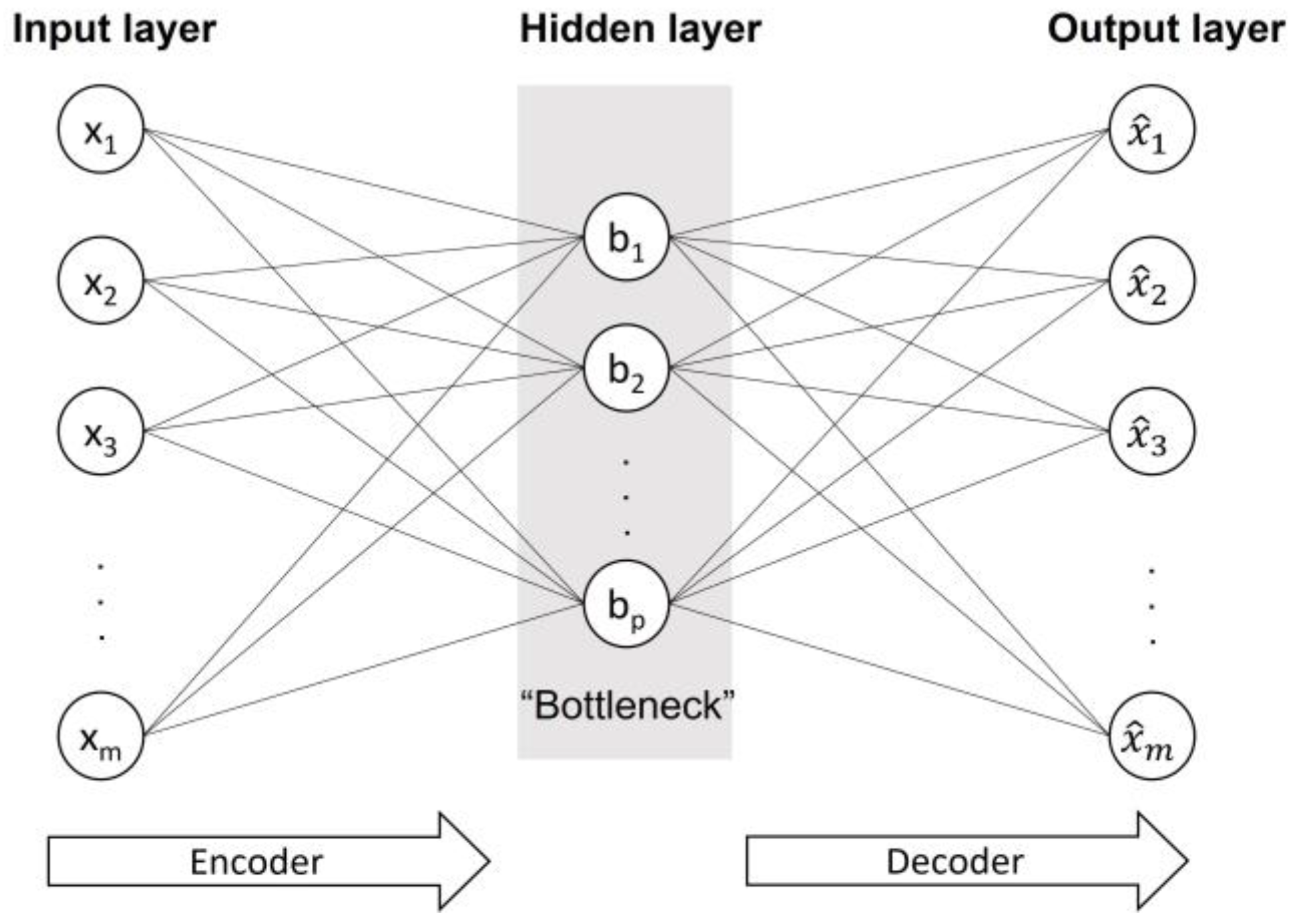
Dimensionality reduction using an autoencoder belongs to unsupervised learning techniques, where the output is not used for learning. In this case, the autoencoder consists of the same number of nodes in the input and output layers, hence corresponding to the first and last layers, respectively. Figure 1 shows an illustration of an autoencoder that consists of the encoder part and decoder part and one hidden layer, which is called the bottleneck layer. The bottleneck layer is often used as the new feature set when using an autoencoder for dimensionality reduction. Although the autoencoder is trained to perform the input-copying task, the bottleneck layer includes salient properties of the dataset, given that its dimension is much smaller than the dimension of the input space. Nevertheless, a drawback for undercomplete autoencoders is that if the width of the encoder and decoder is too large, the autoencoder fails to extract something useful from the dataset.

A simple autoencoder may be either undercomplete or overcomplete. Here, let the original input space be m-dimensional and the bottleneck layer be p-dimensional. Thus, an autoencoder is called undercomplete if p ≪ m, whereas for an overcomplete autoencoder, it would be p ≫ m. An undercomplete autoencoder is ideal for dimensionality reduction tasks because the dimension of the bottleneck layer is smaller than the dimension of the input.

An autoencoder is equivalent to PCA when the encoder and decoder are linear, there is a single hidden layer, and the loss function is the mean squared error. This means that using nonlinear encoder and decoder functions, the autoencoder turns into a nonlinear PCA generalisation. Typical activation functions include the sigmoid function, the hyperbolic tangent (tanh) function, and rectified linear unit (ReLU) and its variants.

Regarding the mathematical formulation of autoencoders, first, the encoder is responsible for the mapping of the input x ϵ ${ℝ}^m$ to a hidden representation h via the activation function f_s. This formulation is presented in Equation (12), as follows:

$$h=f_s\left(Wx+b\right)$$

(12)

where W is an m × m weight matrix and b is a bias vector. On the other hand, the decoder, which is presented in Equation (13), is responsible for the reconstruction of x from the latent representation, hence producing $\widehat{x}$ in the output layer.

$$\widehat{x}=f_s\left(W^{\prime }h+b^{\prime }\right)$$

(13)

where $W^{\prime }$ and $b^{\prime }$ are the parameters of the decoder. The parameters of both the encoder and decoder, namely, $\theta =\left\{W, b\right\}$ and ${\theta }^{\prime }=\left\{W^{\prime },b^{\prime }\right\}$, are estimated based on the minimisation of the average reconstruction error, as shown in Equation (14).

$${\theta }^{*},{\theta }^{\prime *}=\underset{\theta ,{\theta }^{\prime }}{argmin}\frac{1}{n}{\displaystyle \sum }_{i=1}^{n}L\left(x^{\left(i\right)},{\widehat{x}}^{\left(i\right)}\right)$$

(14)

The L function represents the loss function of this algorithm, which is usually the mean squared error $L\left(x,\widehat{x}\right)=\parallel x-\widehat{x}{\parallel }^2$.

3. Support Vector Machine (SVM) for Classification

SVMs [42] are some of the most useful machine learning techniques belonging to supervised techniques. Essentially, an SVM provides a nonprobabilistic predictor used for either classification or regression problems. The goal of an SVM is to map the input space into a higher-dimensional space using nonlinear expressions while also constructing a linear decision boundary to separate the classes in the new feature space. Therefore, the linear decision boundary produced in the feature space is not a straight line in the original input space. Originally, the problem was finding the optimal hyperplane, which is defined by the support vectors, to optimally separate two classes. Consequently, the support vectors are a subset of the training dataset that determines the optimal margins for the separation task.

An SVM is represented by the linear model given in Equation (15), which is similar to logistic regression. However, the difference is that it does not calculate the probabilities, but the output is a class identity [11]:

$$f\left(x\right)=r^T\phi \left(x\right)+d$$

(15)

where φ(x) represents the nonlinear transformation of the input space to the high-dimensional feature space. If the training dataset is represented by (x_i, y_i) pairs, the target values y_i ϵ {−1, 1}, according to the literature, rather than {0, 1}. The SVM predicts the positive class if f is positive and the negative class if f is negative. This means that the SVM classifies input data points based on the sign of f.

The coefficients r and d in Equation (15) are estimated by minimising the regularised risk function (Equation (16)), which serves as the objective function of this problem. This is performed to prevent overfitting and obtain a better generalisation:

$$C{\displaystyle \sum }_{n=1}^N{\xi }_n+\frac{1}{2}\parallel r{\parallel }^2$$

(16)

where C is the regularisation coefficient, which is always positive. C is essentially a hyperparameter, is determined through cross-validation and controls the number of points that are allowed to be misclassified. For C → ∞, the case corresponds to fully separable classes. ξ_n represents non-negative variables, which are called slack variables and have been introduced to provide a soft margin, hence allowing for the misclassification of some of the data points during training. The minimisation problem expressed in Equation (16) can be transformed into a minimisation of the Lagrangian function, which is given in Equation (17) and which takes into account the classification constraints that depend on ξ_n:

$$L\left(r,d,a\right)=\frac{1}{2}\parallel r{\parallel }^2+C{\displaystyle \sum }_{n=1}^N{\xi }_n-{\displaystyle \sum }_{n=1}^N{a}_n\left\{y_{n}f\left(x_n\right)-1+{\xi }_n\right\}-{\displaystyle \sum }_{n=1}^N{\mu }_n{\xi }_n$$

(17)

where $a_n$ and μ_n are non-negative Lagrangian multipliers. Finally, r and d are given in Equations (18) and (19), respectively. Equation (18) shows that vector r corresponds to a linear combination of the support vectors [42]:

$$r={\displaystyle \sum }_{n=1}^N{a}_n{y}_n\varphi \left(x_n\right)$$

(18)

$$d=\frac{1}{N_{ℳ}}{\displaystyle \sum }_{nϵℳ}\left(y_n-{\displaystyle \sum }_{mϵS}{a}_m{y}_{m}K\left(x_n,x_m\right)\right)$$

(19)

where $ℳ$ represents the set of indices of data points, where 0 < a_n < C. The coefficients a_n are calculated by minimising the dual Lagrangian $\tilde{L}$ in Equation (20), which only depends on the coefficients a_n:

$$\tilde{L}\left(a\right)={\displaystyle \sum }_{n=1}^N{a}_n-\frac{1}{2}{\displaystyle \sum }_{n=1}^N{\displaystyle \sum }_{m=1}^N{a}_n{a}_m{y}_n{y}_{m}K\left(x_n,x_m\right)$$

(20)

where $K\left(x_n,x_m\right)=\phi {\left(x_n\right)}^T\phi \left(x_m\right)$. If K represents a kernel function, the technique is called a kernel SVM, transforming the linear SVM into a nonlinear SVM. Common kernel functions are the d^th-degree polynomial kernel (Equation (21)), the radial basis function (RBF) kernel (Equation (22)) and the sigmoid kernel (Equation (23)):

$$K\left(x_n,x_m\right)={\left(x_n{}^T{x}_m+1\right)}^d$$

(21)

$$K\left(x_n,x_m\right)=\exp \left(-\gamma \parallel x_n-x_m{\parallel }^2\right)$$

(22)

$$K\left(x_n,x_m\right)=tanh\left(\gamma x_n{}^T{x}_m+c_0\right)$$

(23)

The hyperparameter γ, which is shown in Equations (22) and (23), is determined through cross-validation. In the case of the RBF kernel, γ = 0.5σ², where σ is the variance.

4. Data Description

The dataset used in the present study is derived from a 10-year-long SCADA dataset of a wind farm located in northwestern Finland. Thus, this dataset has the advantage of including multiple failure events, which typically occur rather rarely. More specifically, the wind farm contains five fixed-speed 2.3 MW wind turbines with a hydraulic pitch system that was commissioned in 2004. The SCADA data are stored in 10 min intervals on average, along with the standard deviation and the maximum and minimum values. A number of measured features are available, but only a subset of them have been selected based on their effect on the hydraulic pitch system [29]. In addition, the present study followed the same methods for preprocessing and labelling the data as those used by Korkos et al. [29]. All of the features presented below have been normalised using min–max normalisation (see Equation (24)) before implementing any data analysis techniques. The result is that the values of the normalised features are between zero and one:

$$x_{new}^i=\frac{x^i-x_{min}}{x_{max}-x_{min}}$$

(24)

where $x^i$ and $x_{new}^i$ are the original and normalised features, respectively, and $x_{min}$ and $x_{max}$ are the minimum and maximum values of each feature, respectively.

Table 1. SCADA feature names and symbols used in this study.

Name	Description	Blade
RS	Rotor speed	-
BAA	Blade angle A	A
BAB	Blade angle B	B
BAC	Blade angle C	C
WS	Wind speed	-
PO	Power output	-
Gust_WS	Gust wind speed	-
HPrA	Hub pressure A	A
HPrB	Hub pressure B	B
HPrC	Hub pressure C	C
HydP	Hydraulic pressure	-
AmbT	Ambient temp.	-
HubT	Hub temp.	-

includes the shortened names of all features, which will be used as labels in the following figures. The features presented in Table 1 are stored as the average, standard deviation, and maximum and minimum values in 10 min intervals, apart from gust wind speed, which contains a single value. At the end of the process, the names of these features, as presented in the figures that follow, will include extensions {‘_mean’, ‘_stdev’, ‘_max’, ‘_min’}, depending on the measured statistical quantity. For instance, if the average value of the rotor speed is mentioned, the shortened name will be ‘RS_mean’. In total, the original input space contains 49 dimensions.

The current paper focuses on a part of the dataset that includes nine pitch events, each one representing a different fault or component of the hydraulic pitch system. During these specific events, the periods before and after those events were gathered and labelled accordingly so as to have normal data points (label = 0) and faulty data points (label = 1). These periods, before and after the failures, are not fixed. They deviate from each other depending on whether a failure in another subsystem occurred quite close to the studied one. Typically, these periods are between 1.5 months and 20 days.

Table 2. Event list.

No.	Pitch Event
1	Hydraulic hoses and oil replacement (WT No1)
2	Hub oil leakage + Hyd. Oil replacement + Bl. valve 6 replacement (WT No4)
3	Block replacement at blade B (WT No3)
4	Block leakage in blade B (WT No1)
5	Replacement of A-blade valve 102 (WT No3)
6	Replacement of A-, B-, C-blade valve 116 (WT No3)
7	Nitrogen accumulator (No4) replacement of Blade A (WT No5)
8	Blade tracking error during stop/operation of Blade A (WT No1)
9	Replacement of hyd. cylinder (WT No2)

summarises the types of events involved in the present research. For example, components that present relatively frequent faults are valves and hydraulic cylinders, as well as common maintenance tasks, such as defects in hydraulic hoses and oils. The text within parentheses in Table 2 refers to the number of wind turbines, out of five, that are included in this study. However, no additional information is presented in this paper due to confidentiality reasons.

5. Model Training and Evaluation Process

The investigated models consisted of a feature extractor to unveil the latent information and an SVM classifier to perform the fault detection task. The best feature extractor among PCA, KPCA and deep autoencoder architectures was determined based on the performance of the SVM classifier, which had the task of using as inputs the new feature set to correctly predict the status of the wind turbine pitch system, that is, normal or faulty. Several other machine learning techniques were tested before using SVMs; these were rejected because of poor performance. More particularly, the rejected classifiers included logistic regression, linear discriminant analysis, k-nearest neighbours and random forests.

To optimise the classifier and prevent overfitting, the hyperparameters ‘C’ and ‘γ’ were tuned through the three-fold cross-validation of a grid search. In addition, optimisation involved the type of SVM kernel, i.e., RBF kernel SVM or linear SVM. The typical values of hyperparameter ‘C’ were {0.01, 0.1, 1, 10, 100, 1000} for both types of SVM classifiers. The ‘γ’ values in the list {0.1, 1, 10, 50, 100, 500} were tested for the case of the RBF SVM classifier. The best performance for all cases was attained using C = 1000 and γ = 10 for an RBF SVM.

After randomly shuffling the dataset, the training of SVM was performed in 80% of the total dataset, while 20% was used to evaluate the SVM performance [11]. The SVM performance was evaluated based on the F1-score, whose expression is given by Equation (25):

$$F1=\frac{2·TP}{2·TP+FP+FN}$$

(25)

where TP is the true positive, implying that the faulty points (label ‘1′) were diagnosed correctly, and FP (false positive) and FN (false negative) are when the normal points and faulty points, respectively, were not predicted correctly.

Other performance metrics, including accuracy, precision and recall, were assumed to provide a limited representation of the performance of this fault detection task. Accuracy was significantly influenced by the large number of normal points compared with the lower number of abnormal points. Thus, missed faulty points were classified as normal, with the accuracy still being high. Precision and recall, which are the fraction of correct detections reported by the model and the fraction of true events that were detected, respectively, could be good evaluation metrics. However, the F1-score was used because it combines the effects of these two scores. Therefore, the goal was to obtain as high an F1-score as possible. A high F1-score indicates that most of the points in the test dataset were predicted correctly.

6. Results and Discussion

6.1. Feature Extractors and SVM Performance

The first feature extraction technique that was utilised was PCA, which is based on a linear transformation of the input space. The first two PCs accounted for 83.2% of the cumulative explained variance, but when using only the first two PCs, the normal and faulty points were not clearly separated into two clusters. Consequently, nonlinear relationships existed, and more PCs were needed. Therefore, the selection of the number of PCs was based on a threshold regarding the cumulative explained variance, which was set arbitrarily. In the current study, a 95% threshold was used, which is a common value for scientists.

Figure 2 demonstrates the cumulative explained variance after increasing the number of PCs each time. In general, PCA produces as many PCs as the number of original input spaces. Because 49 features were available, 49 PCs were extracted, ending up at 100% cumulative explained variance if all of these were taken into consideration. However, 95% of the cumulative explained variance corresponded to the selection of the first seven PCs. Thus, the reduced 7D output space was assumed to be the one accounting for most of the structure in the data after PCA.

Figure 3 visualises the 2D subplots of each PC against a different PC when referring only to the first seven PCs. The axes labels in Figure 3 include the explained variance of the visualised PC in brackets, in addition to the number of the particular PC. The blank subplots refer to ones in which the input variable is plotted against itself, which would not make sense to visualise. Figure 3 shows that no single 2D representation presented an obvious separation between normal and faulty classes. Moreover, their dependence was nonlinear. Therefore, a more sophisticated feature extraction based on nonlinear relationships needed to be investigated.

The second feature extraction technique is similar to PCA, but the kernel trick was used to implement a nonlinear transformation of the original input space. More specifically, in the present study, an RBF kernel, also known as Gaussian, was used that is based on standard normal density. The Gaussian kernel was selected because it tends to give good performance under general smoothness assumptions [43]. The representation of the first two principal components, as derived by the RBF kernel PCA, demonstrated the poor separation of the two classes in the space of the first principal components. Therefore, more principal components were needed, as in the PCA case. For this reason, the first seven principal components, as given by the RBF kernel PCA, were used for further investigation as the new input space, as in PCA. In addition, the hyperparameter γ = 1.0 was chosen based on the cross-validation of the SVM performance.

The third approach belongs to the deep learning field and is called an autoencoder. An autoencoder is a type of neural network that attempts to reconstruct the original input space with as little information leakage as possible; it deploys a nonlinear transformation using nonlinear activation functions between layers. The current study investigated multiple architectures of an autoencoder, whose architectures and results are presented briefly in

Table 3. F1-scores of fault detection using SVM for different extracted feature sets.

Feature Extractor	Dimension of New Feature Set	SVM Kernel	Activation Function	F1-Score
Original feature set	-	RBF	-	0.8538
2D PCA	2	RBF	-	0.7195
7D PCA	7	RBF	-	0.7713
2D RBF PCA	2	RBF	-	0.7388
7D RBF PCA	7	RBF	-	0.8519
Deep Autoencoder [n,32,16,8,2,8,16,32,n]	2	RBF	ReLU	0.4353
Deep Autoencoder [n,32,16,8,8,8,16,32,n]	8	RBF	ReLU	0.7679
Deep Autoencoder [n,32,16,8,8,8,16,32,n]	8	RBF	Sigmoid	0.5979
Deep Autoencoder [n,32,8,32,n]	8	RBF	ReLU	0.7845
Deep Autoencoder [n,32,8,32,n]	8	RBF	Sigmoid	0.9548

. If n is the number of input spaces, n = 49 in the current study. Almost all of the investigated architectures had an 8D code layer, except for the one with a 2D code layer. As for the activation functions, sigmoid and ReLU were investigated. The examined architectures were trained for 10,000 epochs with a batch size of 64. The loss function was the mean squared error (MSE), and the Adam algorithm was also used as an optimisation algorithm. The selection of the architecture was based on the performance of an SVM classifier, whose training process is described in detail in Section 5.

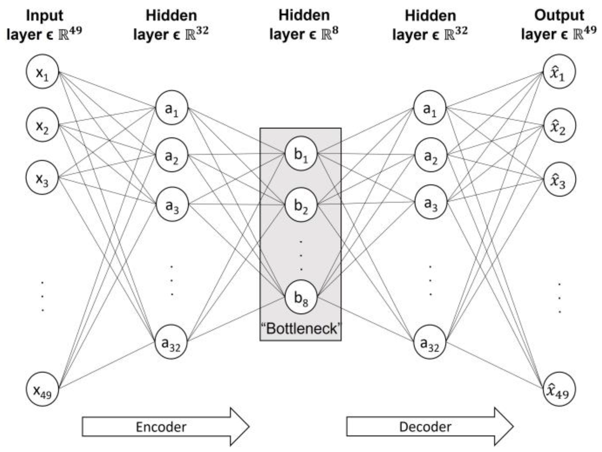
Table 3 summarises the F1-scores of the SVM using either the original feature set or the new features extracted by the PCA, kernel PCA using RBF and deep autoencoder. More specifically, it includes the dimensions of the new feature sets for each case, the type of kernel for the SVM classifier and the activation function of the deep autoencoders. The deep autoencoders are accompanied by their architectures, i.e., the number of neurons for each layer. The results clearly show that the deep autoencoder [n,32,8,32,n], which is shown in Figure 4 and has eight dimensions in the latent space while using a sigmoid function as the activation function, was the best compared with the other four autoencoder architectures, PCA and kernel PCA. More specifically, it attained almost a 95.5% F1-score and proved that fault detection using a feature extracted by a nonlinear dimensionality reduction technique can perform better than using only the original feature set. In fact, the developed architecture of the aforementioned deep autoencoder increased the performance of the SVM by a notable amount of 11.8%. Other architectures using either the same number of hidden layers and units or more did not perform better than using the original feature set. This situation is expected because if the encoder and decoder are given too much capacity, the undercomplete autoencoder fails to learn anything useful [11].

Regarding PCA and its kernel version, linearly transformed features using PCA showed that by increasing the number of components, that is, from two to seven dimensions, which accounted for 95% of the cumulative explained variance, a better F1-score was obtained, but it was not sufficient to justify the usefulness of feature extraction for fault detection. Using seven PCs rather than two demonstrated a 7.2% increase in the F1-score. Similar results were presented for the case of a kernel PCA but without providing much better performance for the SVM.

The F1-score of 95.5% performance of the developed model, here using the latent dimensions of the deep autoencoder [n,32,8,32,n], outperformed the performance of the ANFIS presented in Korkos et al. [29]. Other approaches in the literature do not allow us to directly compare their results with those of the present study because of dataset variability. However, in a relevant study by Leahy et al. [33], the fault detection task attained a 65% F1-score, without showing more details about the faults. Furthermore, Hu et al. [34] managed to test their model and achieved a 90% F1-score when enhancing the feature set. Finally, Chen et al. [27] evaluated their trained ANFIS model by achieving a 50% F1-score for fixed-speed wind turbines using some pitch faults but provided no information about them. Consequently, the attained F1-score using autoencoder-extracted features led to the conclusion that autoencoders can extract useful information from the dataset while providing more distinguishable patterns of system faults.

6.2. Physical Interpretation of Autoencoder-Extracted Features

In this subsection, the features extracted by the deep autoencoder [n,32,8,32,n] are interpreted physically to show the usefulness of this approach and its practical outcome. This analysis is based on the mutual information between the original features, which were stored in SCADA, and the new features that have been extracted by the deep autoencoder [n,32,8,32,n]. Mutual information [41] is a measure of the dependence between two random variables and has been used in the current study to demonstrate that each new extracted feature is mostly affected by a different combination of the original features. In other words, mutual information can unveil how these new extracted features can capture the differences between different faulty signals regarding the nature of each fault, which, here, is a fault either in the hydraulic cylinder or in a valve. The mutual information between two random variables X and Y is given by Equation (26):

$$I\left(X,Y\right)={\displaystyle \sum }_{yϵY}{\displaystyle \sum }_{xϵX}p\left(x,y\right)log\frac{p\left(x,y\right)}{p\left(x\right)p\left(y\right)}$$

(26)

where p(x) and p(y) are the marginal density functions of X and Y, respectively, and p(x,y) is the joint probability density function of X and Y. I is also called the Kullback–Leibler divergence between the joint distribution and the product of the marginals [10]. I(X,Y) is always non-negative, and if X and Y are independent, then I(X,Y) is zero. As a result, the dependence between the two random variables is revealed by as much mutual information as possible.

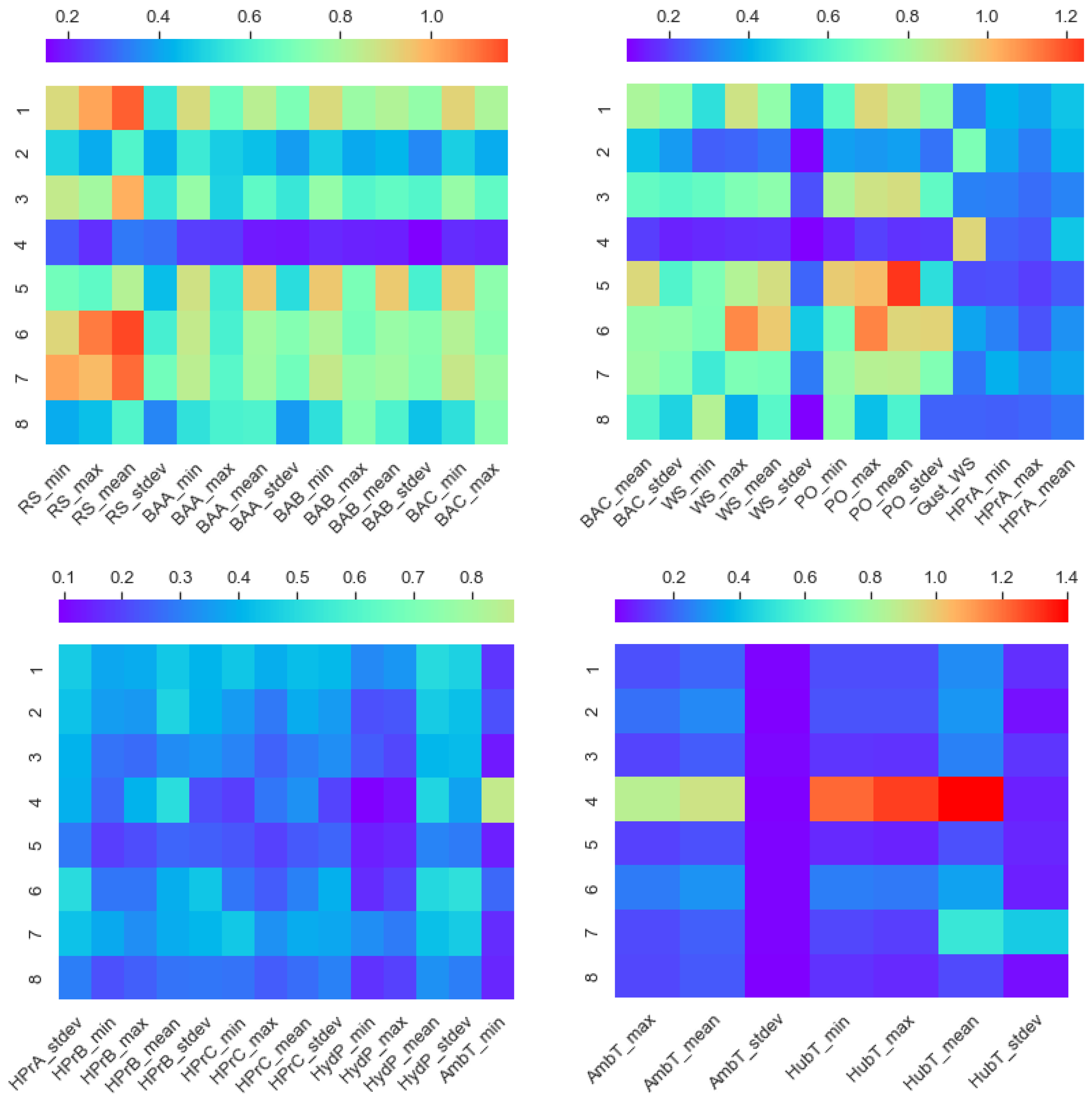
Figure 5 shows the mutual information map between each original feature (horizontal axis) and each dimension of the latent space (vertical axis) of the developed model (autoencoder [n,32,8,32,n]). This map provides details about the dependencies between the original and extracted features. The strongest effect is marked with red colour, whereas the weakest effect is marked with violet colour, as shown in the colour bars of Figure 5. Therefore, for features that have the highest mutual information scores, this implies that those features had the largest effect on the new extracted features.

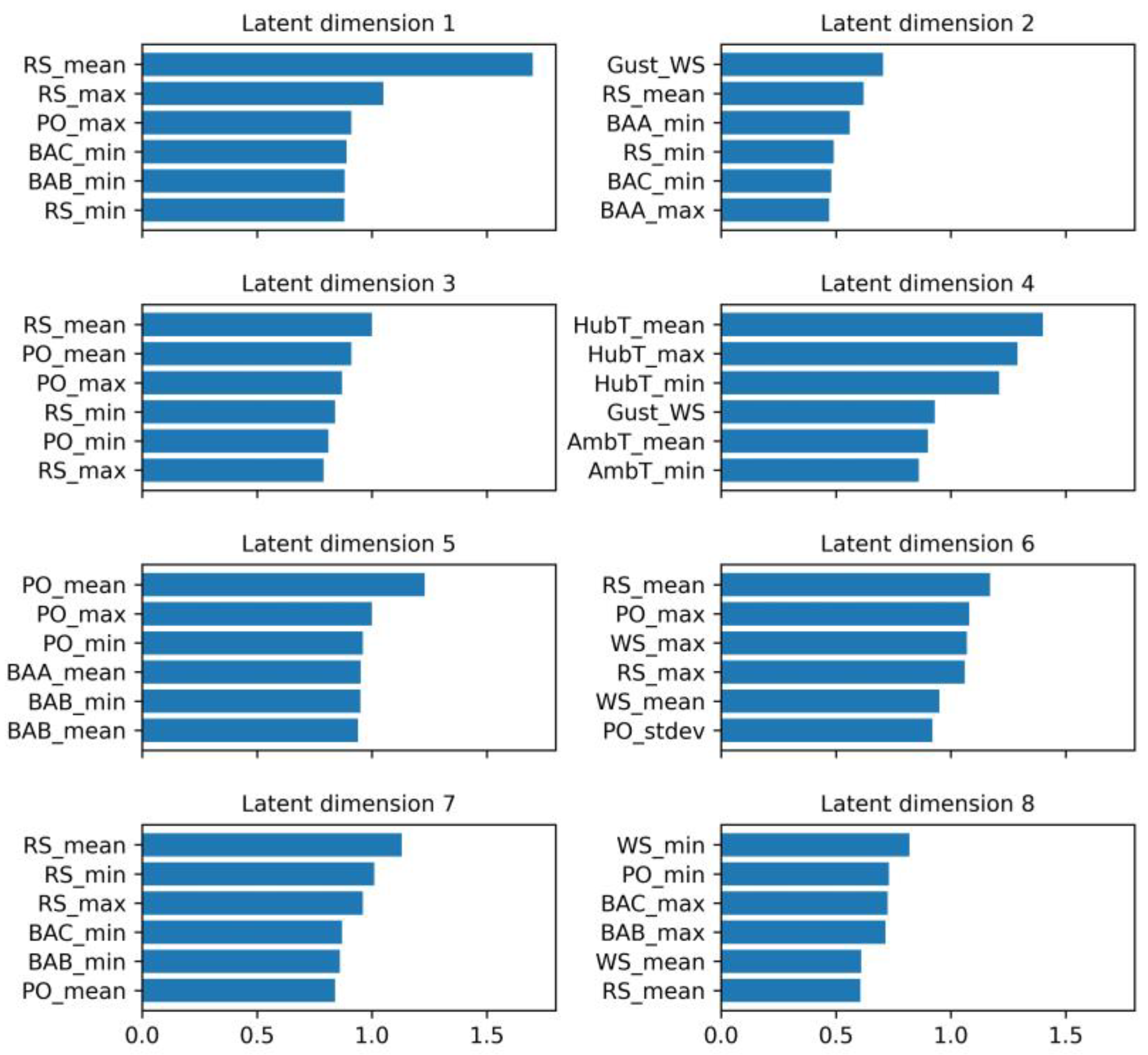
For instance, the average hub temperature had the highest dependency on the fourth latent dimension. The average rotor speed had the highest impact on the first, third, sixth and seventh latent dimensions, whereas the gust wind speed and minimum wind speed had the largest effect on the second and eighth dimensions, respectively. Latent dimension 5 was mostly influenced by the average power output. The top six features that had the greatest influence on each latent dimension are presented in Figure 6. These figures make it more obvious that almost all of the new extracted features depend mostly on the critical characteristic features (CCFs) [27,29], namely, power output, wind speed, the three blade angles and the rotor speed, save for the fourth latent dimension.

In general, hydraulic pressures on either the hub or pump station seemed to have the lowest influence among all of the new extracted features. In the same group, the least influential features were also the standard deviation of the ambient temperature and hub temperature. This is why the blue colour is observed throughout all latent dimensions in Figure 5. On the contrary, all of the new extracted features had a clear dependency with the rest of the 49 features, except for the case of the 4th latent dimension. Regarding the fourth latent dimension, it mostly depended on the gust wind speed, hub temperature, including the average, minimum and standard deviation, and ambient temperature, including the average, minimum and standard deviation.

Multiple latent dimensions, particularly the first, third, fifth, sixth and seventh extracted features, demonstrated strong dependency with most of the original features, proving that the information contained in these signals was encoded in multiple dimensions of the new extracted feature set. Fault detection and identification saw a benefit due to this because the impact of faults was encoded in multiple latent dimensions, allowing for more distinguishable patterns of specific faults.

7. Conclusions

In the current work, PCA, kernel PCA and autoencoder were applied for feature extraction to test their performance on the fault detection of a wind turbine hydraulic pitch system. SVMs were used as classifiers to compare their impacts. The main objective was to test whether the final configurations of the above-mentioned techniques can attain better SVM performance than using the original feature set. In the present paper, the available feature set contained 49 dimensions, ranging from the power output and rotor speed to several pressures and temperatures in the hydraulic pitch system of wind turbines. Linear transformations of the original input space were represented by PCA, and nonlinear transformations were represented by kernel PCA and an autoencoder. The dataset included nine pitch events, each one representing a different pitch fault, such as a valve fault and a hydraulic cylinder fault. SVM was trained on 80% of the dataset, and 20% was used for testing. Hyperparameter tuning was performed using three-fold cross-validation.

The results show that the features extracted by the deep autoencoder with one ${ℝ}^{32}$ hidden layer for the encoder and decoder and one ${ℝ}^8$ as the code dimension not only outperformed the traditional PCA and kernel PCA but also performed better than using only the original features. The achieved F1-score using autoencoder-extracted features was almost 95.5%, which was 11.8% larger than using only the original feature set. This conclusion proves the power of an undercomplete autoencoder in extracting information under the assumption that data would be concentrated around a low-dimensional manifold or a small set of such manifolds. In addition, the final architecture of the undercomplete autoencoder seemed to conform to the general rule that if the encoder and decoder are given too much capacity, they will fail to learn anything useful.

Although autoencoder-extracted features significantly outperformed the original ones in the context of fault detection (binary classification task) when using an SVM, regularised autoencoders may be investigated in the future because they can allow for more capacity. Regularised autoencoders include sparse autoencoders and denoising autoencoders, which are suitable for the fault detection task. In particular, regularised ones fix the problem of depth by using a loss function that allows the model to have properties other than copying the input to its output. Furthermore, possible future research includes the use of a different classifier from the deep learning area, such as a 1D convolutional neural network or long short-term memory network (LSTM), which will be trained based on the same autoencoder-extracted features.