
A Novel Temperature-Independent Model for Estimating the Cooling Energy in Residential Homes for Pre-Cooling and Solar Pre-Cooling

 , , ,
, , ,
Abstract
1. Introduction
1.1. Existing Research on Pre-Cooling
1.2. Existing Research on Solar Pre-Cooling
1.3. Paper Contribution
2. AccuRate
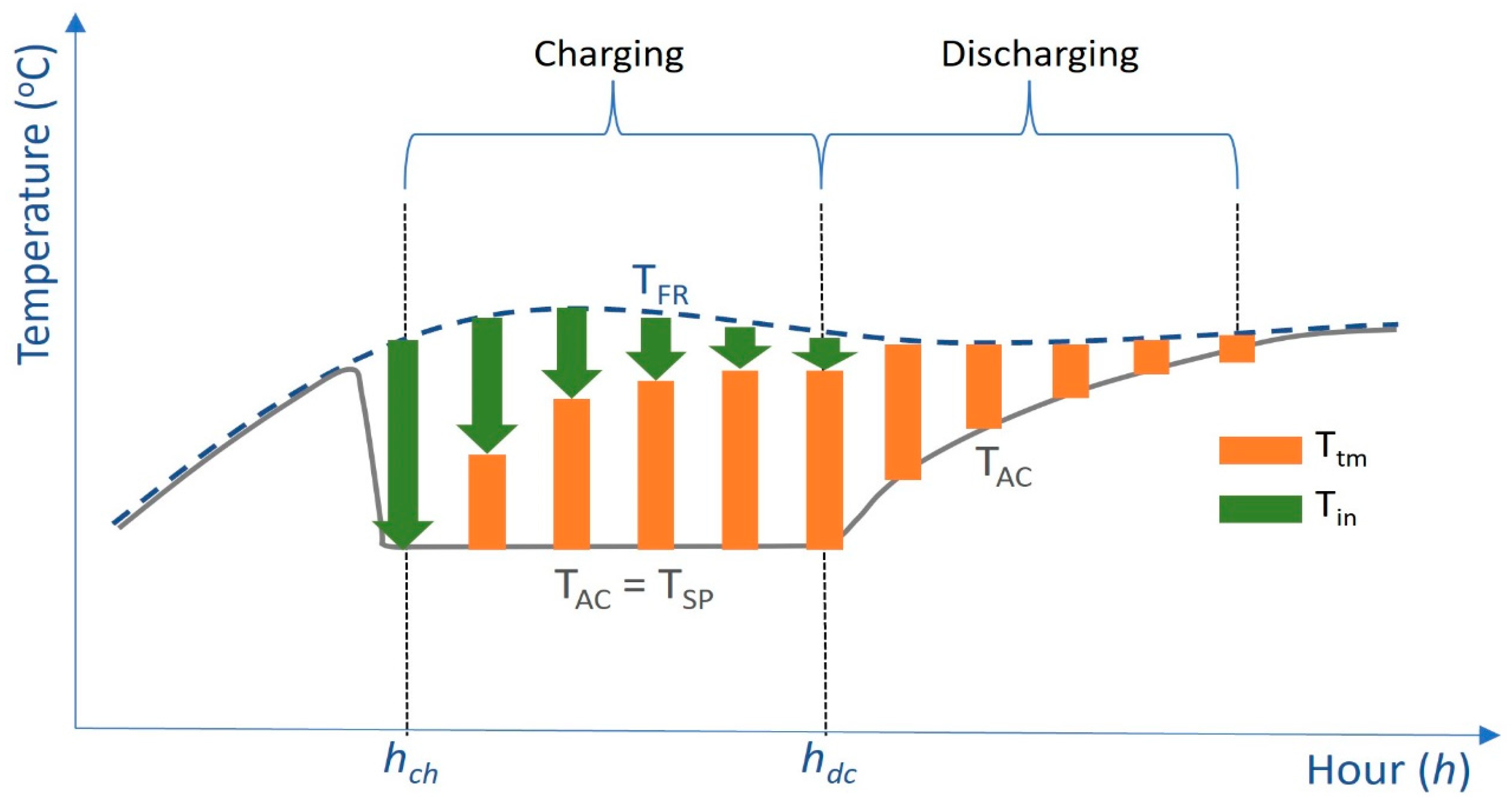
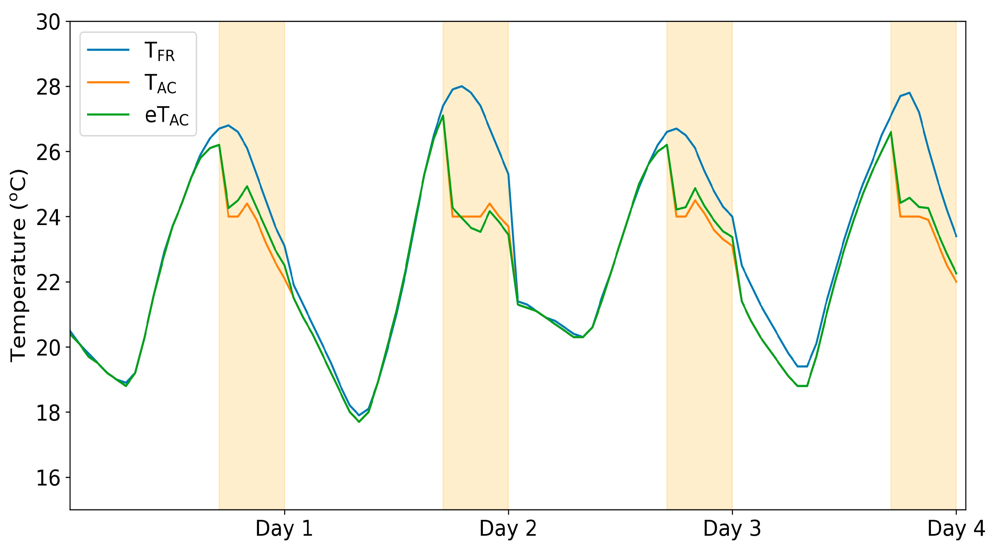
- TFR (°C) is the free running temperature, i.e., the indoor temperature with no AC;
- TAC (°C) is the air conditioned temperature, i.e., the indoor temperature where AC is controlled to maintain thermal comfort using a temperature setpoint; and
- EEin (kWh) is the electrical energy consumed by the AC unit.
3. Method
3.1. Linear Equations
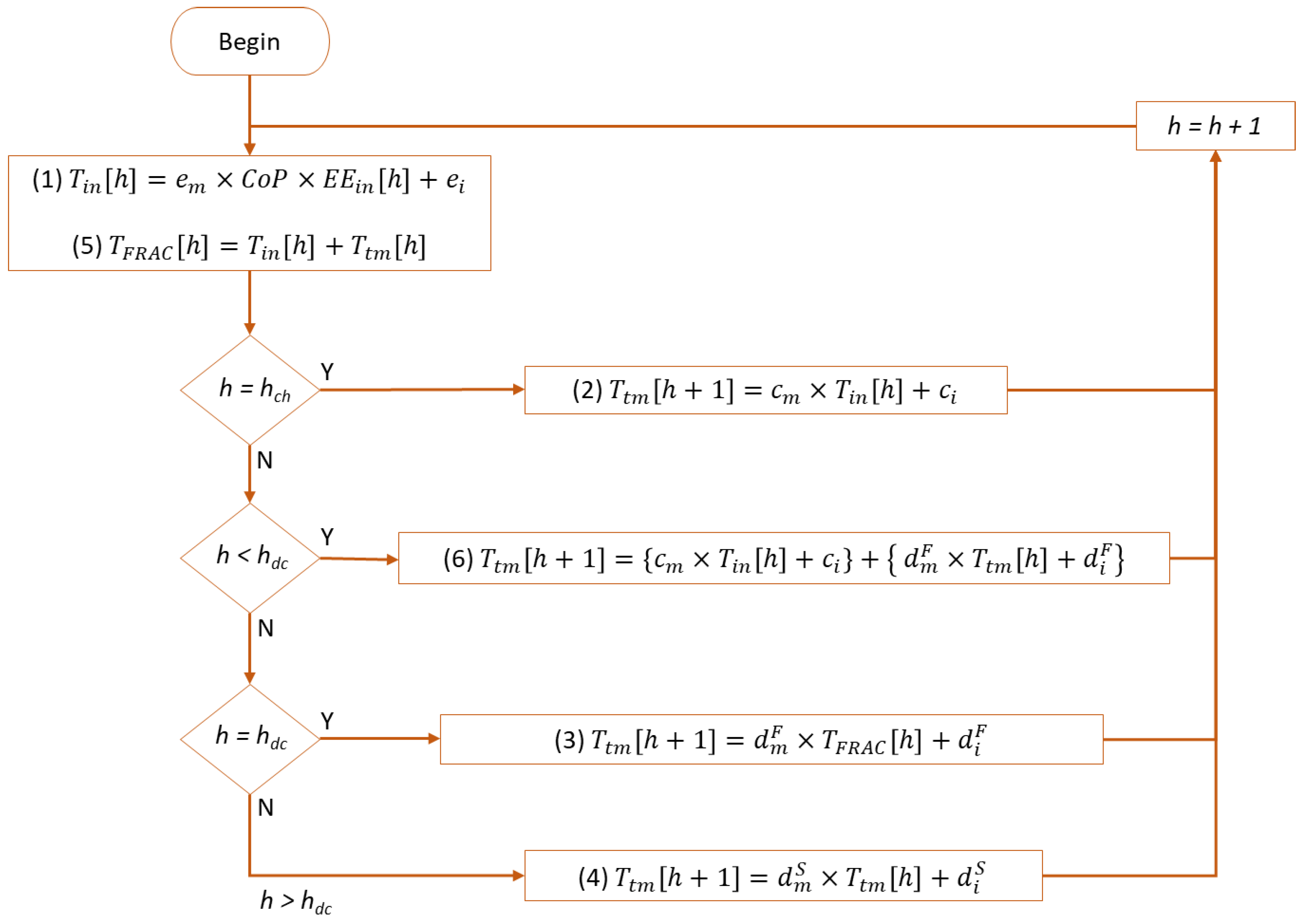
3.2. Implementation of the Model
- (1)
- The sum of Tin and Ttm equals TFRAC, as defined by Equation (5):
- (2)
- Equation (1) can be used to calculate Tin at any hour h.
- (3)
- During the charging phase, the thermal dynamics of the home are assumed to operate in accordance with Equation (6):
4. Results
5. Model Significance
6. Conclusions
- Extending the model to solar pre-heating;
- An analysis of the potential of solar pre-cooling using measured residential energy data to examine the impact of build type, climate, and different solar pre-cooling control and optimisation algorithms to reduce peak demand, increase minimum demand, and reduce electricity costs;
- The development of proof to explain the strong R2 values for the thermal metrics; and
- The development of a model to derive the thermal metrics of a building from its energy data.
Supplementary Materials
Author Contributions
Funding
Data Availability Statement
Acknowledgments
Conflicts of Interest
Nomenclature
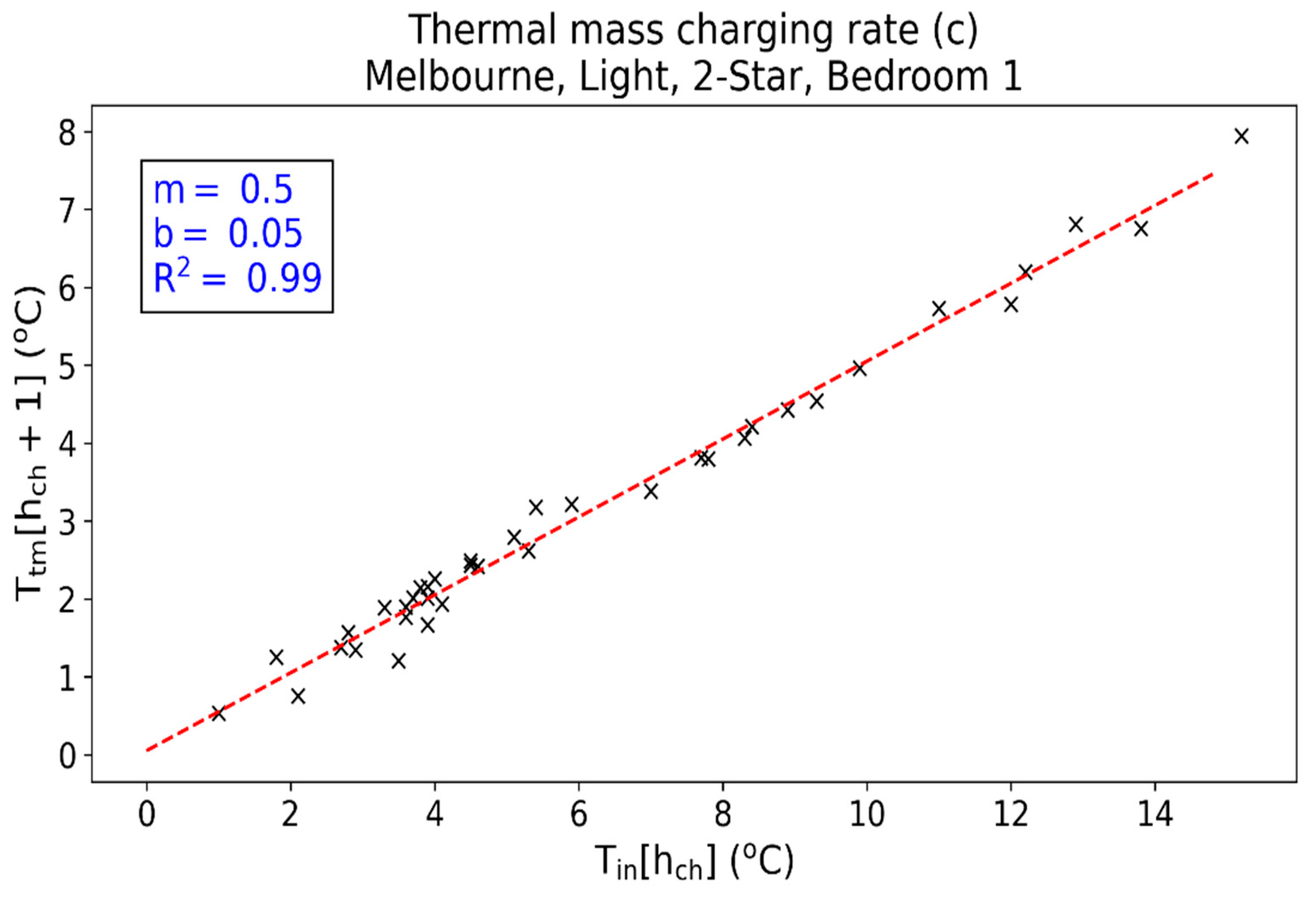
| c | is the thermal mass charging rate |
| cm | is the slope of the thermal mass charging rate (c) |
| ci (°C) | is the intercept of the thermal mass charging rate (c) |
| CoP | is the coefficient of performance of the AC unit |
| CV-RMSE (%) | is the Coefficient of the Variation of the Root Mean Square Error |
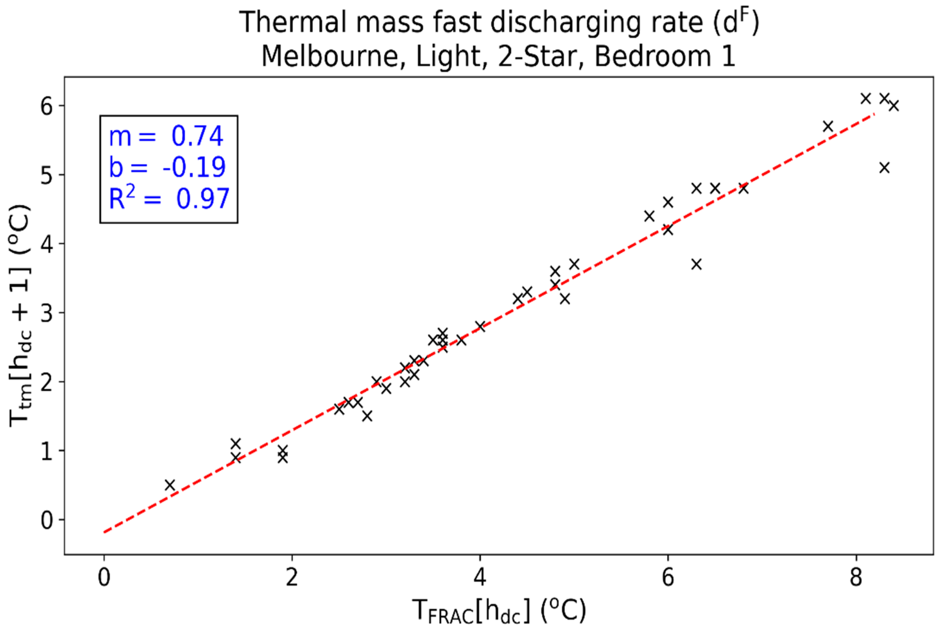
| dF | is the thermal mass fast discharging rate |
| is the slope of the thermal mass fast discharging rate (dF) | |
| (°C) | is the intercept of the thermal mass fast discharging rate (dF) |
| dS | is the thermal mass slow charging rate |
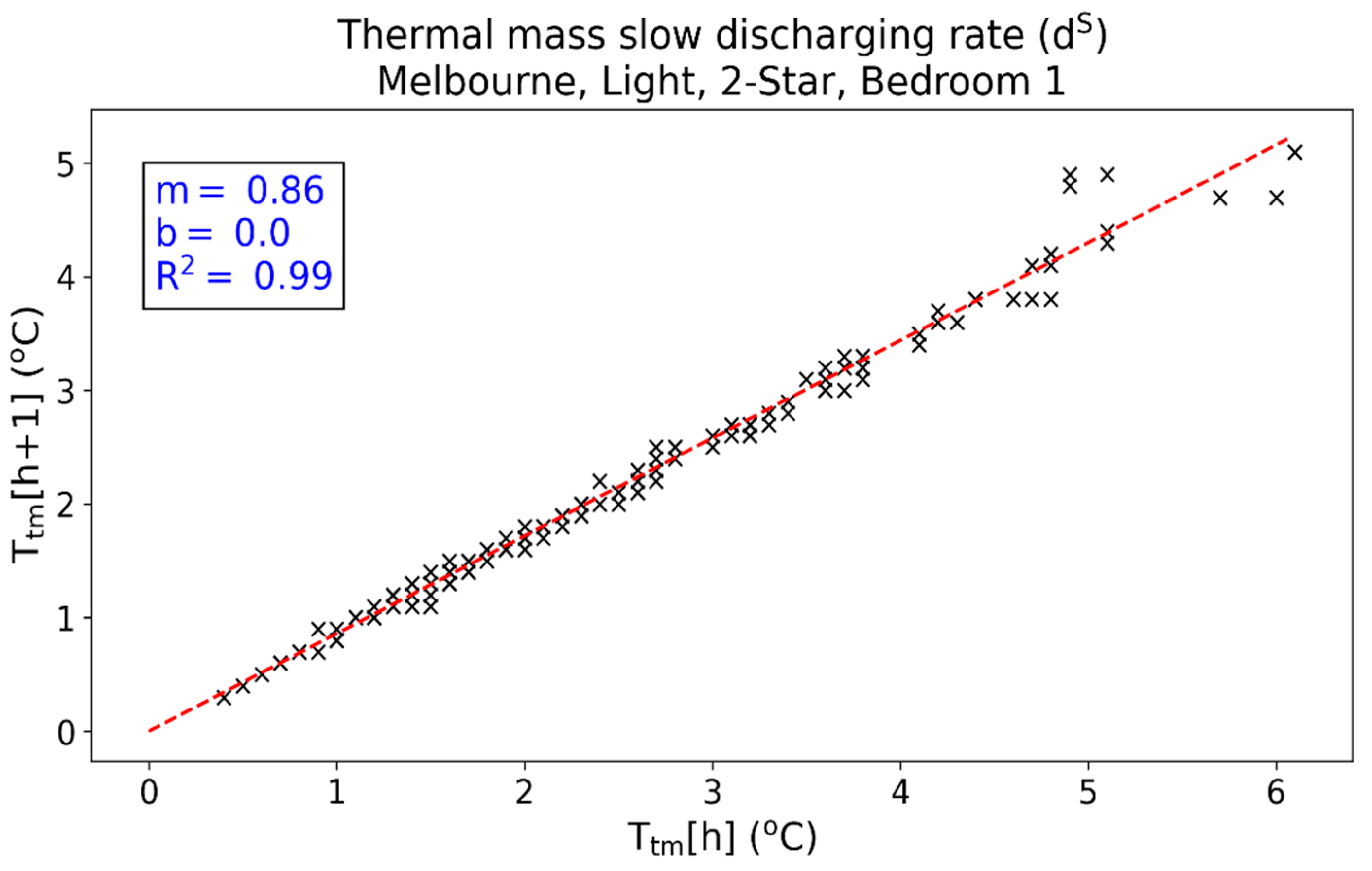
| is the slope of the thermal mass slow discharging rate (dS) | |
| (°C) | is the intercept of the thermal mass slow discharging rate (dS) |
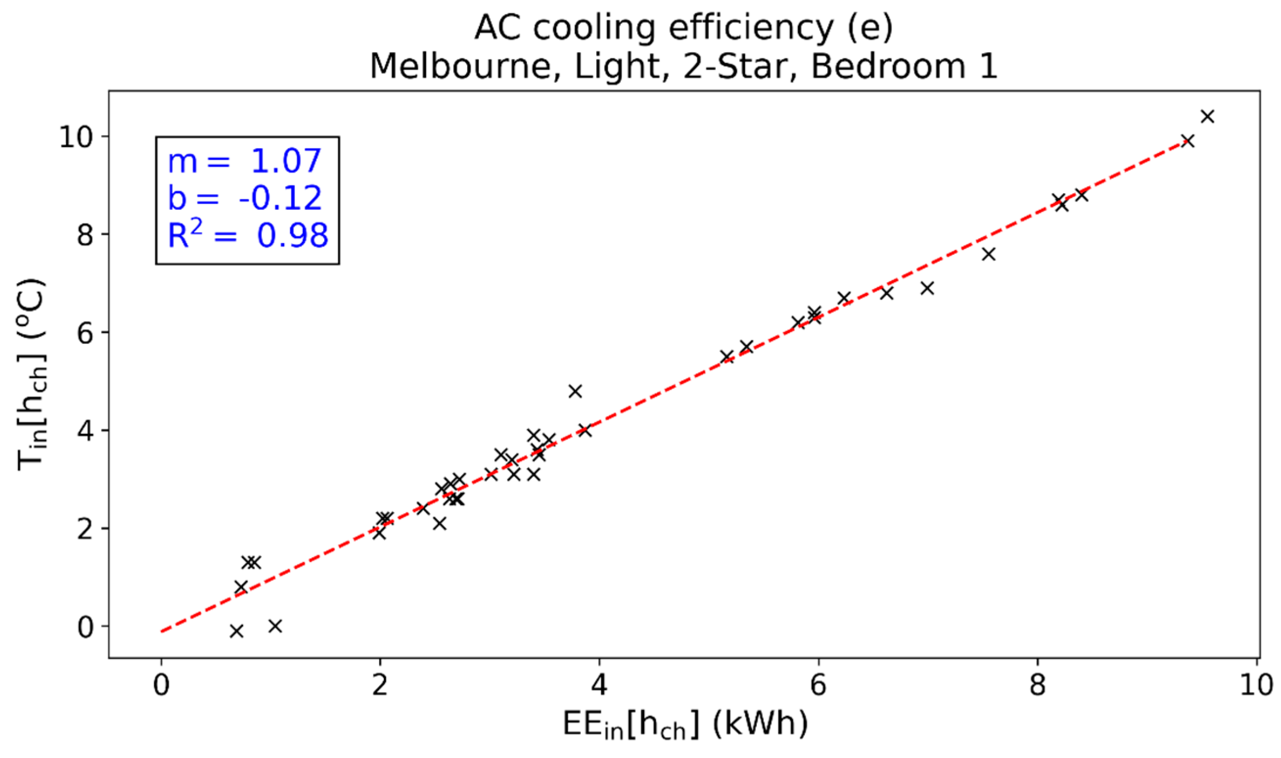
| e | is the AC cooling efficiency |
| em (°C/kWh) | is the slope of the AC cooling efficiency (e) |
| ei (°C) | is the intercept of the AC cooling efficiency (e) |
| EEin (kWh) | is the electrical energy consumed by the AC unit |
| (kWh) | is the equivalent electrical energy consumed by the AC unit to attain Ttm |
| hch | is the first hour of the charging phase |
| hdc | is the first hour of the discharging phase |
| MAE (°C) | is the Mean Absolute Error |
| R2 | is the coefficient of determination |
| TAC (°C) | is the air conditioned temperature. |
| TFR (°C) | is the free running temperature, the indoor temperature with no air conditioning. |
| TFRAC (°C) | is the difference between TFR and TAC. |
| Tin (°C) | represents the temperature difference due to cooling energy injected into the thermal zone by the AC unit |
| Ttm (°C) | represents the temperature difference due to the cooling energy stored in the thermal mass |
Appendix A
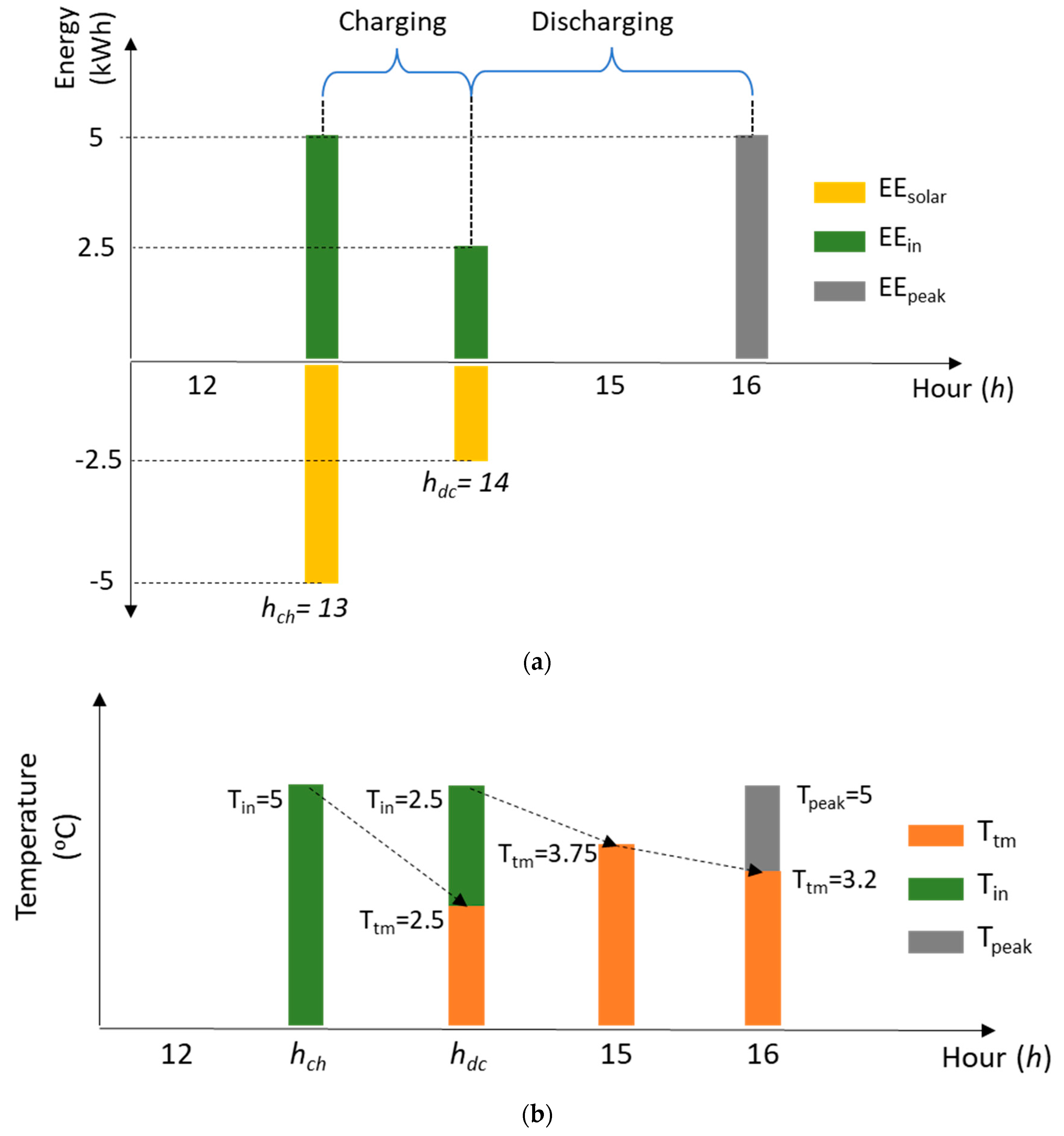
Solar Pre-Cooling Example


| h = hch | h = hdc | |
| Tin[h] | ||
| Ttm[h] | 0 | 2.5 |
| TFRAC[h] | ||
| Ttm[h + 1] | ||
| h = 15 | h = 16 | |
| Tin[h] | 0 | 0 |
| Ttm[h] | 3.75 | 3.2 |
| TFRAC[h] | ||
| Ttm[h + 1] |
| Template Home | City | AC Cooling Efficiency (e) | ||
|---|---|---|---|---|
| em (°C/kWh) | ei (°C) | R2 | ||
| B2L | Brisbane | 1.38 | −0.15 | 0.91 |
| B2M | 1.24 | −0.11 | 0.94 | |
| B2H | 1.03 | −0.01 | 0.95 | |
| B6L | 1.40 | −0.08 | 0.93 | |
| B6M | 1.39 | −0.08 | 0.91 | |
| B6H | 0.90 | −0.05 | 0.88 | |
| S2L | Sydney | 1.45 | −0.46 | 0.90 |
| S2M | 1.24 | −0.08 | 0.96 | |
| S2H | 0.80 | −0.02 | 0.93 | |
| S6L | 1.39 | −0.11 | 0.94 | |
| S6M | 1.36 | −0.14 | 0.89 | |
| S6H | 0.94 | −0.12 | 0.83 | |
| M2L | Melbourne | 1.22 | −0.31 | 0.98 |
| M2M | 1.22 | −0.28 | 0.98 | |
| M2H | 0.81 | −0.11 | 0.98 | |
| M6L | 1.36 | −0.41 | 0.97 | |
| M6M | 1.31 | −0.22 | 0.97 | |
| M6H | 0.89 | −0.17 | 0.93 | |
| A2L | Adelaide | 1.41 | −1.10 | 0.93 |
| A2M | 1.16 | −0.25 | 0.97 | |
| A2H | 0.81 | 0.02 | 0.99 | |
| A6L | 1.45 | −0.65 | 0.96 | |
| A6M | 1.37 | −0.46 | 0.94 | |
| A6H | 0.85 | −0.18 | 0.89 | |
| Template Home | City | Thermal Mass Charging Rate (c) | ||
|---|---|---|---|---|
| cm | ci (°C) | R2 | ||
| B2L | Brisbane | 0.78 | 0.06 | 0.91 |
| B2M | 0.32 | 0.39 | 0.82 | |
| B2H | 0.40 | 0.15 | 0.86 | |
| B6L | 0.90 | 0.07 | 0.99 | |
| B6M | 0.46 | 0.44 | 0.83 | |
| B6H | 0.60 | 0.20 | 0.88 | |
| S2L | Sydney | 0.50 | 0.59 | 0.95 |
| S2M | 0.40 | 0.31 | 0.94 | |
| S2H | 0.35 | 0.27 | 0.69 | |
| S6L | 0.76 | 0.32 | 0.93 | |
| S6M | 0.48 | 0.54 | 0.81 | |
| S6H | 0.53 | 0.30 | 0.81 | |
| M2L | Melbourne | 0.53 | 0.38 | 0.99 |
| M2M | 0.41 | 0.14 | 0.96 | |
| M2H | 0.36 | 0.09 | 0.87 | |
| M6L | 0.62 | 0.39 | 0.93 | |
| M6M | 0.50 | 0.32 | 0.94 | |
| M6H | 0.27 | 0.37 | 0.80 | |
| A2L | Adelaide | 0.55 | 0.70 | 0.97 |
| A2M | 0.50 | −0.34 | 0.95 | |
| A2H | 0.63 | −0.70 | 0.91 | |
| A6L | 0.77 | −0.61 | 0.94 | |
| A6M | 0.62 | −0.27 | 0.90 | |
| A6H | 0.82 | −1.52 | 0.90 | |
| Template Home | City | Thermal Mass Fast Discharging Rate (dF) | ||
|---|---|---|---|---|
| (°C) | R2 | |||
| B2L | Brisbane | 0.53 | 0.24 | 0.86 |
| B2M | 0.58 | 0.10 | 0.84 | |
| B2H | 0.67 | 0.07 | 0.81 | |
| B6L | 0.74 | 0.12 | 0.90 | |
| B6M | 0.68 | 0.10 | 0.87 | |
| B6H | 0.67 | 0.06 | 0.88 | |
| S2L | Sydney | 0.62 | 0.02 | 0.92 |
| S2M | 0.63 | 0.09 | 0.95 | |
| S2H | 0.67 | 0.07 | 0.87 | |
| S6L | 0.67 | 0.29 | 0.90 | |
| S6M | 0.75 | 0.06 | 0.93 | |
| S6H | 0.74 | 0.00 | 0.88 | |
| M2L | Melbourne | 0.76 | −0.21 | 0.97 |
| M2M | 0.63 | −0.09 | 0.95 | |
| M2H | 0.75 | −0.15 | 0.97 | |
| M6L | 0.87 | −0.31 | 0.97 | |
| M6M | 0.81 | −0.14 | 0.97 | |
| M6H | 0.73 | −0.12 | 0.85 | |
| A2L | Adelaide | 0.86 | −1.05 | 0.93 |
| A2M | 0.71 | −0.44 | 0.90 | |
| A2H | 0.79 | −0.41 | 0.97 | |
| A6L | 0.95 | −1.11 | 0.96 | |
| A6M | 0.80 | −0.45 | 0.92 | |
| A6H | 0.85 | −0.73 | 0.87 | |
| Template Home | City | Thermal Mass Slow Discharging Rate (dS) | ||
|---|---|---|---|---|
| (°C) | R2 | |||
| B2L | Brisbane | 0.92 | −0.04 | 0.99 |
| B2M | 0.85 | 0.00 | 0.97 | |
| B2H | 0.90 | −0.03 | 0.97 | |
| B6L | 0.96 | −0.04 | 0.99 | |
| B6M | 0.92 | −0.01 | 0.98 | |
| B6H | 0.95 | −0.04 | 0.98 | |
| S2L | Sydney | 0.91 | −0.01 | 0.99 |
| S2M | 0.82 | 0.03 | 0.98 | |
| S2H | 0.94 | −0.04 | 0.98 | |
| S6L | 0.96 | −0.03 | 1.00 | |
| S6M | 0.92 | 0.00 | 0.99 | |
| S6H | 0.98 | −0.06 | 0.99 | |
| M2L | Melbourne | 0.86 | 0.00 | 0.99 |
| M2M | 0.84 | −0.04 | 0.98 | |
| M2H | 0.94 | −0.05 | 1.00 | |
| M6L | 0.93 | 0.02 | 1.00 | |
| M6M | 0.92 | −0.04 | 1.00 | |
| M6H | 0.97 | −0.06 | 1.00 | |
| A2L | Adelaide | 0.88 | 0.05 | 0.99 |
| A2M | 0.87 | −0.04 | 0.98 | |
| A2H | 0.96 | −0.08 | 0.99 | |
| A6L | 0.95 | 0.01 | 1.00 | |
| A6M | 0.90 | −0.02 | 0.99 | |
| A6H | 0.97 | −0.06 | 1.00 | |
References
- International Energy Association. IEA PVPS Snapshot. 2020. Available online: https://iea-pvps.org/snapshot-reports/snapshot-2020/ (accessed on 5 July 2022).
- Australian Energy Market Operator. Advice to Commonwealth Government on Dispatchable Capability. 2017. Available online: https://www.aemo.com.au/-/media/Files/Media_Centre/2017/Advice-To-Commonwealth-Government-On-Dispatchable-Capability.PDF (accessed on 5 July 2022).
- Australian Energy Market Operator. Renewable Integration Study: Stage 1 Report. 2020. Available online: https://aemo.com.au/-/media/files/major-publications/ris/2020/renewable-integration-study-stage-1.pdf?la=en (accessed on 5 July 2022).
- Centre for Energy and Environmental Markets, University of New South Wales. Voltage Analysis of the LV Distribution Network in the Australian National Electricity Market. 2020. Available online: https://prod-energycouncil.energy.slicedtech.com.au/lv-voltage-report (accessed on 5 July 2022).
- International Renewable Energy Agency. Future of Solar Photovoltaic. 2019. Available online: https://www.irena.org/-/media/Files/IRENA/Agency/Publication/2019/Nov/IRENA_Future_of_Solar_PV_2019.pdf (accessed on 8 July 2022).
- Distributed Energy Resources. 2018. Available online: https://arena.gov.au/funding/distributed-energy-resources/ (accessed on 8 July 2022).
- Olsthoorn, D.; Haghighat, F.; Moreau, A.; Lacroix, G. Abilities and limitations of thermal mass activation for thermal comfort, peak shifting and shaving: A review. Build. Environ. 2017, 118, 113–127. [Google Scholar] [CrossRef]
- Roberts, M.B.; Bruce, A.; MacGill, I. Impact of shared battery energy storage systems on photovoltaic self-consumption and electricity bills in apartment buildings. Appl. Energy 2019, 245, 78–95. [Google Scholar] [CrossRef]
- Keeney, K.R.; Braun, J.E. Application of Building Precooling to Reduce Peak Cooling Requirements; ASHRAE Transactions: Atlanta, GA, USA, 1997; Volume 103, pp. 463–469. [Google Scholar]
- Rabl, A.; Norford, L. Peak Load Reduction by Preconditioning Buildings at Night. Int. J. Energy Res. 1991, 15, 781–798. [Google Scholar] [CrossRef]
- Braun, J.E. Load control using building thermal mass. J. Sol. Energy Eng. 2003, 125, 292–301. [Google Scholar] [CrossRef]
- Lee, K.H.; Braun, J.E. Model-based demand-limiting control of building thermal mass. Build. Environ. 2008, 43, 1633–1646. [Google Scholar] [CrossRef]
- Yin, R.; Xu, P.; Piette, M.A.; Kiliccote, S. Study on Auto-DR and pre-cooling of commercial buildings with thermal mass in California. Energy Build. 2010, 42, 967–975. [Google Scholar] [CrossRef]
- Rijksen, D.; Wisse, C.; van Schijndel, A. Reducing peak requirements for cooling by using thermally activated building systems. Energy Build. 2010, 42, 298–304. [Google Scholar] [CrossRef]
- Xu, P.; Haves, P.; Piette, M.A. Peak Demand Reduction from Pre-Cooling with Zone Temperature Reset in an Office Building; Purdue University: Purdue, IN, USA, 2006. [Google Scholar]
- Turner, W.; Walker, I.; Roux, J. Peak load reductions: Electric load shifting with mechanical pre-cooling of residential buildings with low thermal mass. Energy 2015, 82, 1057–1067. [Google Scholar] [CrossRef]
- Ramos, J.S.; Moreno, M.P.; Delgado, M.G.; Domínguez, S.Á.; Cabeza, L.F. Potential of energy flexible buildings: Evaluation of DSM strategies using building thermal mass. Energy Build. 2019, 203, 109442. [Google Scholar] [CrossRef]
- Hu, M.; Xiao, F.; Wang, L. Investigation of demand response potentials of residential air conditioners in smart grids using grey-box room thermal model. Appl. Energy 2017, 207, 324–335. [Google Scholar] [CrossRef]
- Korkas, C.D.; Baldi, S.; Michailidis, I.; Kosmatopoulos, E.B. Intelligent energy and thermal comfort management in grid-connected microgrids with heterogeneous occupancy schedule. Appl. Energy 2015, 149, 194–203. [Google Scholar] [CrossRef]
- O’Shaughnessy, E.; Cutler, D.; Ardani, K.; Margolis, R. Solar plus: Optimization of distributed solar PV through battery storage and dispatchable load in residential buildings. Appl. Energy 2018, 213, 11–21. [Google Scholar] [CrossRef]
- Nelson, J.; Johnson, N.G.; Chinimilli, P.T.; Zhang, W. Residential cooling using separated and coupled precooling and thermal energy storage strategies. Appl. Energy 2019, 252, 113414. [Google Scholar] [CrossRef]
- Ice Energy Brings the Deep Freeze to U.S. Energy Storage. 2019. Available online: https://pv-magazine-usa.com/2019/02/13/ice-energy-brings-the-deep-freeze-to-u-s-energy-storage/ (accessed on 8 July 2022).
- Saurav, K.; Bansal, H.; Nawhal, M.; Chandan, V.; Arya, V. Minimizing energy costs of commercial buildings in developing countries. In Proceedings of the 2016 IEEE International Conference on Smart Grid Communications (SmartGridComm), Sydney, Australia, 6–9 November 2016; pp. 637–642. [Google Scholar]
- Arababadi, R.; Parrish, K. Reducing the Need for Electrical Storage by Coupling Solar PVs and Precooling in Three Residential Building Types in the Phoenix Climate; ASHRAE Transactions: Atlanta, GA, USA, 2017; Volume 123. [Google Scholar]
- Romaní, J.; Belusko, M.; Alemu, A.; Cabeza, L.F.; de Gracia, A.; Bruno, F. Control concepts of a radiant wall working as thermal energy storage for peak load shifting of a heat pump coupled to a PV array. Renew. Energy 2018, 118, 489–501. [Google Scholar] [CrossRef]
- Seem, J.E. Modeling of Heat Transfer in Buildings; The University of Wisconsin-Madison: Madison, WI, USA, 1987. [Google Scholar]
- Romaní, J.; Belusko, M.; Alemu, A.; Cabeza, L.F.; de Gracia, A.; Bruno, F. Optimization of deterministic controls for a cooling radiant wall coupled to a PV array. Appl. Energy 2018, 229, 1103–1110. [Google Scholar] [CrossRef]
- Calero, I.; Cañizares, C.A.; Bhattacharya, K.; Baldick, R. Duck-Curve Mitigation in Power Grids with High Penetration of PV Generation; IEEE Transactions on Smart Grid: Piscataway, NJ, USA, 2021; Volume 13, pp. 314–329. [Google Scholar]
- Smart Residential Load Simulator. 2021. Available online: https://uwaterloo.ca/power-energy-systems-group/downloads/smart-residential-load-simulator-srls (accessed on 15 September 2022).
- Wang, H.; Good, N.; Mancarella, P. Modelling and valuing multi-energy flexibility from community energy systems. In 2017 Australasian Universities Power Engineering Conference (AUPEC); IEEE: Piscataway, NJ, USA, 2017. [Google Scholar]
- Perez, K.X.; Baldea, M.; Edgar, T.F. Integrated HVAC management and optimal scheduling of smart appliances for community peak load reduction. Energy Build. 2016, 123, 34–40. [Google Scholar] [CrossRef]
- AccuRate: Helping Designers Deliver Energy Efficient Homes. 2020. Available online: https://www.csiro.au/en/Research/EF/Areas/Grids-and-storage/Intelligent-systems/AccuRate (accessed on 15 September 2022).
- Nationwide House Energy Rating Scheme. 2020. Available online: https://www.nathers.gov.au/ (accessed on 15 September 2022).
- A Validation of the AccuRATE Simulation Engine Using BESTEST. 2004. Available online: https://www.nathers.gov.au/sites/default/files/Validation%2520of%2520the%2520AccuRate%2520Simulation%2520Engine%2520Using%2520BESTEST_0.pdf (accessed on 15 September 2022).
- Judkoff, R.; Neymark, J. International Energy Agency Building Energy Simulation Test (BESTEST) and Diagnostic Method; National Renewable Energy Lab. (NREL): Golden, CO, USA, 1995. [Google Scholar]
- Household Census Data. 2021. Available online: https://quickstats.censusdata.abs.gov.au/census_services/getproduct/census/2016/quickstat/1GSYD?opendocument (accessed on 22 July 2022).
- NatHERS Administrator. Nationwide House Energy Rating Scheme (NatHERS)—Software Accreditation Protocol; Department of Environment and Energy: Canberra, Australia, 2012. [Google Scholar]
- Law, A. Building Evaluation: The decay Method as an Evaluation Tool for Analysing Thermal Performance. Ph.D. Thesis, RMIT University, Melbourne, VIC, Australia, 2018. [Google Scholar]
- Guideline, A. Measurement of Energy, Demand, and Water Savings; ASHRAE Guidel: Atlanta, GA, USA, 2014; Volume 4, pp. 1–150. [Google Scholar]


| Template Home | City | Climate | Build Type | Walls | Windows | Floors | Ceilings | |
|---|---|---|---|---|---|---|---|---|
| Star Rating | Build Weight | |||||||
| B2L | Brisbane | Humid Subtropical | 2 | Light | R0 | SG | R0 | R0 |
| B2M | Medium | R0 | SG | R0 | R0.1 | |||
| B2H | Heavy | R0 | SG | R0 | R0.4 | |||
| B6L | 6 | Light | R0 | SG | R0 | R4 | ||
| B6M | Medium | R0.7 | DG | R0 | R4 | |||
| B6H | Heavy | R2.3 | DG | R2.5 | R5 | |||
| S2L | Sydney | Humid Subtropical | 2 | Light | R0 | SG | R0 | R0 |
| S2M | Medium | R0 | SG | R0 | R0 | |||
| S2H | Heavy | R0 | SG | R0 | R0.5 | |||
| S6L | 6 | Light | R1.3 | SG | R0 | R4 | ||
| S6M | Medium | R0.9 | DG | R0 | R4 | |||
| S6H | Heavy | R2.5 | DG | R3 | R5 | |||
| M2L | Melbourne | Temperate | 2 | Light | R0 | SG | R0 | R0.1 |
| M2M | Medium | R0 | SG | R0 | R0.1 | |||
| M2H | Heavy | R0 | SG | R0 | R0 | |||
| M6L | 6 | Light | R2 | SG | R0 | R4 | ||
| M6M | Medium | R1.1 | DG | R0 | R4 | |||
| M6H | Heavy | R1.4 | DG | R3 | R4 | |||
| A2L | Adelaide | Mediterranean | 2 | Light | R0 | SG | R0 | R0 |
| A2M | Medium | R0 | SG | R0 | R0.1 | |||
| A2H | Heavy | R0 | SG | R0 | R0.3 | |||
| A6L | 6 | Light | R0.4 | SG | R0 | R2.5 | ||
| A6M | Medium | R0.7 | DG | R0 | R4 | |||
| A6H | Heavy | R2 | DG | R3 | R4 | |||
| Template Home | City | CV-RMSE (%) | MAE (°C) | Air Conditioning Days |
|---|---|---|---|---|
| B2L | Brisbane | 19.18 | 0.21 | 63 |
| B2M | 19.74 | 0.22 | 62 | |
| B2H | 22.08 | 0.24 | 91 | |
| B6L | 14.99 | 0.15 | 29 | |
| B6M | 22.33 | 0.21 | 52 | |
| B6H | N/A | N/A | 3 | |
| S2L | Sydney | 20.43 | 0.25 | 21 |
| S2M | 21.91 | 0.23 | 27 | |
| S2H | N/A | N/A | 8 | |
| S6L | N/A | N/A | 7 | |
| S6M | 21.82 | 0.25 | 15 | |
| S6H | N/A | N/A | 5 | |
| M2L | Melbourne | 23.1 | 0.3 | 13 |
| M2M | 16.76 | 0.28 | 13 | |
| M2H | N/A | N/A | 3 | |
| M6L | 18.79 | 0.31 | 12 | |
| M6M | N/A | N/A | 5 | |
| M6H | N/A | N/A | 2 | |
| A2L | Adelaide | 26.53 | 0.44 | 20 |
| A2M | 25.77 | 0.43 | 24 | |
| A2H | N/A | N/A | 7 | |
| A6L | 28.12 | 0.57 | 12 | |
| A6M | 26.65 | 0.42 | 18 | |
| A6H | N/A | N/A | 8 |
Publisher’s Note: MDPI stays neutral with regard to jurisdictional claims in published maps and institutional affiliations. |
© 2022 by the authors. Licensee MDPI, Basel, Switzerland. This article is an open access article distributed under the terms and conditions of the Creative Commons Attribution (CC BY) license (https://creativecommons.org/licenses/by/4.0/).
Share and Cite
Heslop, S.; Yildiz, B.; Roberts, M.; Chen, D.; Lau, T.; Naderi, S.; Bruce, A.; MacGill, I.; Egan, R. A Novel Temperature-Independent Model for Estimating the Cooling Energy in Residential Homes for Pre-Cooling and Solar Pre-Cooling. Energies 2022, 15, 9257. https://doi.org/10.3390/en15239257
Heslop S, Yildiz B, Roberts M, Chen D, Lau T, Naderi S, Bruce A, MacGill I, Egan R. A Novel Temperature-Independent Model for Estimating the Cooling Energy in Residential Homes for Pre-Cooling and Solar Pre-Cooling. Energies. 2022; 15(23):9257. https://doi.org/10.3390/en15239257
Chicago/Turabian StyleHeslop, Simon, Baran Yildiz, Mike Roberts, Dong Chen, Tim Lau, Shayan Naderi, Anna Bruce, Iain MacGill, and Renate Egan. 2022. "A Novel Temperature-Independent Model for Estimating the Cooling Energy in Residential Homes for Pre-Cooling and Solar Pre-Cooling" Energies 15, no. 23: 9257. https://doi.org/10.3390/en15239257
APA StyleHeslop, S., Yildiz, B., Roberts, M., Chen, D., Lau, T., Naderi, S., Bruce, A., MacGill, I., & Egan, R. (2022). A Novel Temperature-Independent Model for Estimating the Cooling Energy in Residential Homes for Pre-Cooling and Solar Pre-Cooling. Energies, 15(23), 9257. https://doi.org/10.3390/en15239257