Data Compensation with Gaussian Processes Regression: Application in Smart Building’s Sensor Network

Abstract

Data play an essential role in the optimal control of smart buildings’ operation, especially in building energy-management for the target of nearly zero buildings. The building monitoring system is in charge of collecting and managing building data. However, device imperfections and failures of the monitoring system are likely to produce low-quality data, such as data loss and inconsistent data, which then seriously affect the control quality of the buildings. This paper proposes a new approach based on Gaussian process regression for data-quality monitoring and sensor network data compensation in smart buildings. The proposed method is proven to effectively detect and compensate for low-quality data thanks to the application of data analysis to the energy management monitoring system of a building model in Viet Nam. The research results provide a good opportunity to improve the efficiency of building energy-management systems and support the development of low-cost smart buildings.

1. Introduction

Buildings are the biggest consumer of 40% of energy consumption and are responsible for 36% of CO₂ pollution worldwide [1]. Therefore, efficient monitoring and control of buildings’ energy demands and renewable energy integration provide an excellent opportunity to reduce energy consumption and CO₂ emissions, leading to smart building technology development. Smart buildings technology applies advanced techniques in machine learning and automatic control to optimize building energy consumption and production while guaranteeing user comfort and building security [2].

Smart buildings use monitoring systems that include a massive number of sensors to collect data from the environment, such as temperature, humidity, lighting, power production, and power consumption of multiple zones in the building. These data are essential for energy modeling, analysis, forecasting, energy audit, and user comfort evaluation.

Traditionally, building monitoring systems were costly and required expert knowledge (hardware and software), which made them only affordable to large commercial buildings [3]. However, the fast development of low-cost IoT technologies and open-source hardware programming provided an opportunity to build low-cost monitoring systems applicable to small and medium-scale buildings [3]. In an emerging country such as Vietnam, the research on smart buildings is in its early stages and should be based on such low-cost sensor networks.

Unfortunately, a low-cost monitoring system occasionally produces inconsistent data and losses of data due to device malfunction and communication failure [4]. Fault sensors in the network are one of the main obstacles to addressing sensor networks in the practical.

Those might cause a delay in real-time energy management or mistaken control actions that results in low performance of the building’s energy behavior.

Traditionally, calibrating sensors is not feasible in large-scale sensor networks at large scale; however, in many cases, smart buildings’ applications need more precise measurements than the low cost that uncalibrated sensors provide. Therefore, the field’s methods of automatically calibrating sensor networks are of great interest.

Features such as data quality and completeness (i.e., data compensation and virtual sensors) and sensor maintenance procedures (i.e., sensor fault detection and sensor calibration) in low-cost monitoring systems are inevitable requirements to improve the modeling accuracy and increase the reliability of the building control.

Models based on data and machine-learning techniques will give great value for optimal control of future buildings. Virtual sensors are predictive models that provide several properties, such as:

-

Lower cost than expensive hardware devices, allowing for more comprehensive monitoring networks;

-

They can work in parallel with physical sensors, providing helpful information for fault-detection tasks, thus enabling more reliable control processes;

-

They can be easily implemented on existing hardware (e.g., microcontrollers) and be updated as system parameters change.

Despite the significance of data-quality monitoring in smart buildings, most research on smart buildings only focuses on technical costs [3,5], user behaviors [6,7,8], and prediction [6,7] and control [9,10,11]. There has been no dedicated approach for data compensation in smart-building applications. Research on data compensation in smart buildings still remains a literature gap.

The issues of data compensation and virtual sensors have been seriously addressed in environmental applications such as air-quality monitoring over a city/country, in which the measurements of several locations’ air quality by low-cost sensors are used to infer air-quality data at the other locations.

The researchers typically employ neural network models such as the nonlinear auto-regressive exogenous model (NARX) and long short-term memory model (LSTM) [12,13,14], and statistical models such as Gaussian process regression (GPR) [15].

In [15], Gaussian process regression is proven to give accurate results in estimating air pollution at a location in which monitoring stations are unavailable from the air pollution measured at other places. Gaussian process regression has some substantial advantages over neural network methods, i.e., it provides an explicit uncertainty measure that helps to quantify the confidence of the measurement, and it does not necessitate the same lengthy ‘training’ as a neural network [16].

In the literature review, GPR models can also contribute to the control solutions. For example, the GPR models are applied in MPC, such as a linear predictive controller [17,18,19] and a nonlinear predictive controller [20]. The characteristics of the dataset related to the quality of the predictive models include data length, sampling frequency, quantity and variety of data, and data quality [21]. The approaches to speed up the standard GPR prediction time are noted in [22,23]. The potential of GPR in predictive Solar Radiation Forecasting models has been shown in [24].

In [25], the GPR approach is proved effective at developing an online GHI model. However, the research depends on the availability of data from a high-resolution weather station, which is sometimes unavailable in all areas.

This paper presents a method to exploit the richness of sensor nodes for data-quality monitoring and data compensation in smart buildings. The data loss and inconsistent data at a sensor node can be detected and compensated based on the data at other nodes. Gaussian process regression is selected to train models and generate the compensation. In this study, our aims include:

-

Evaluating the suitability of GPR in the different datasets of sensor nodes in the building.

-

Evaluating the ability to detect data errors and compensate data based on the correlation of the available data of the sensor nodes in a building and shared building data in the local area.

-

Evaluating the computational performance of the model considering the data size for online models, which can participate in the building management system in smart buildings, smart grids, etc.

Section 2 presents the infrastructure and the roles of a building monitoring system, as well as its existing issues. Section 3 proposes a new method to handle the issues. Section 4 evaluates the proposed method’s performance with real experiments and discussions, and Section 5 concludes the paper.

2. Building Monitoring Systems: Infrastructure and Functions

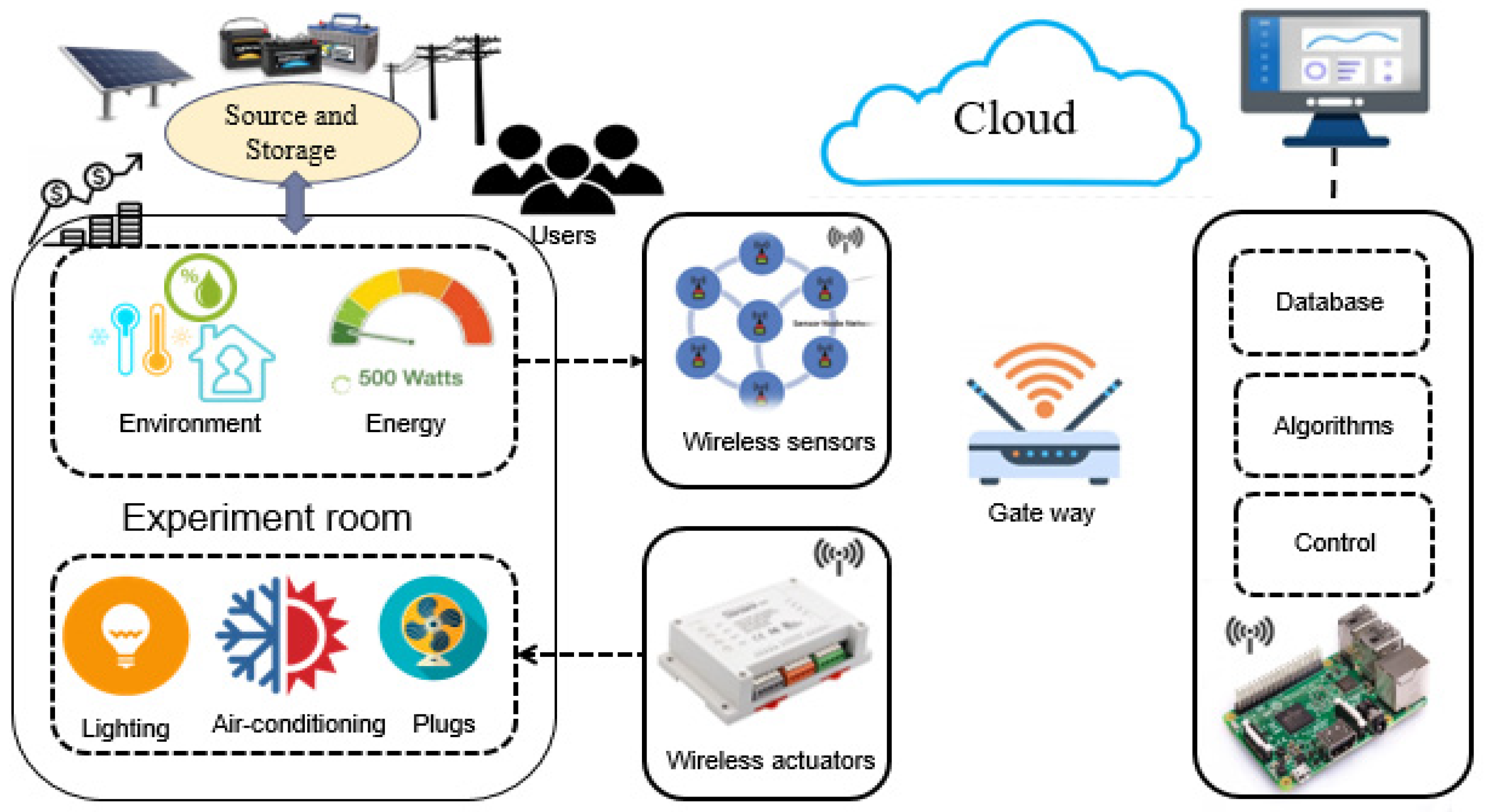
As shown in Figure 1, a building monitoring system is mainly composed of a sensors network used to collect the building data: a number of actuators equipped with communication ability to remotely regulate the building’s devices, gateways, and database storage systems (cloud, local servers, etc.).

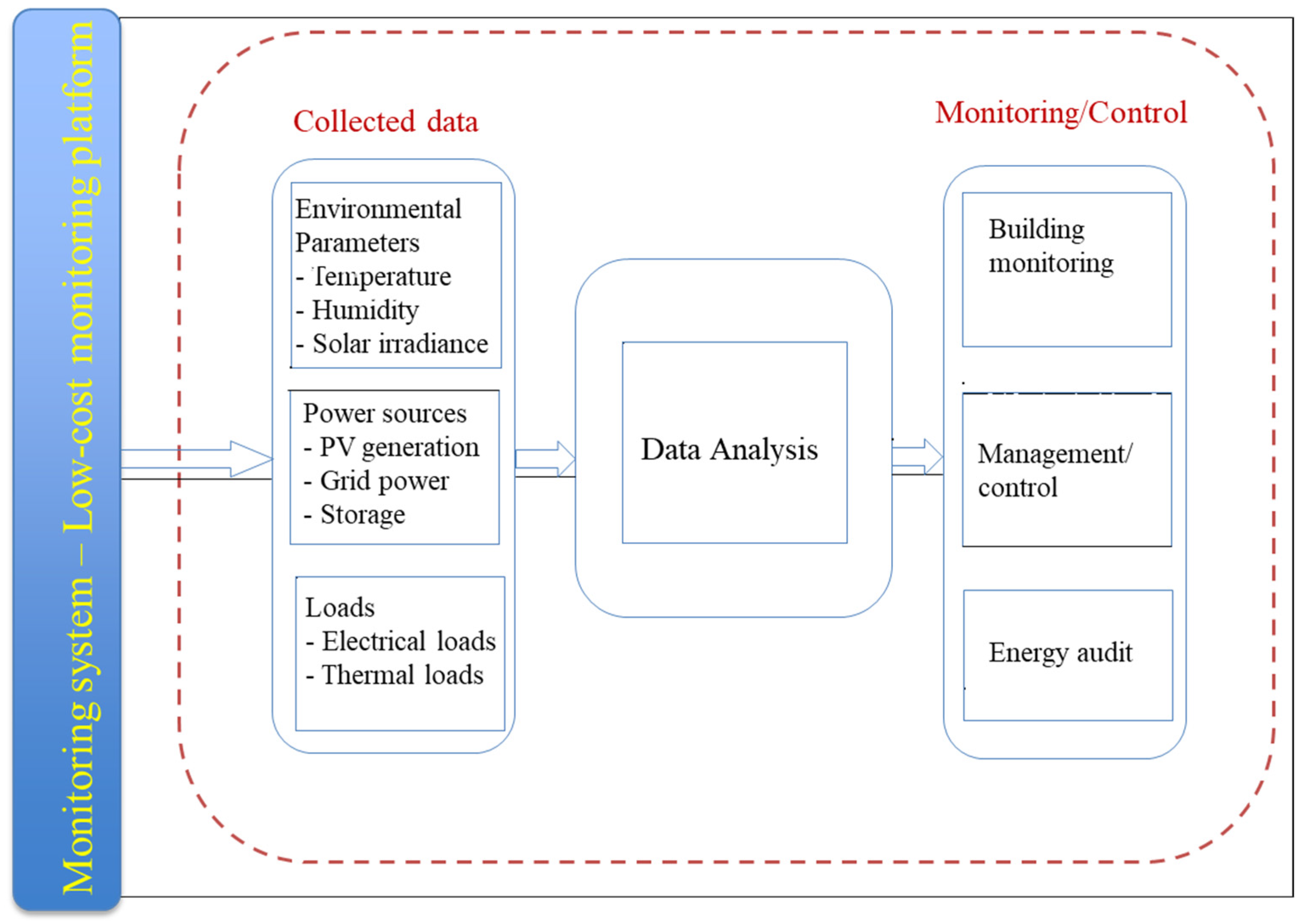
A building monitoring system plays a central role in building energy-management. As in Figure 2, the building monitoring system collects the following information:

• Environmental parameters: solar irradiance, indoor and outdoor temperature, humidity, and air quality of multiple zones of the building.
• HVAC parameters: hot/chilled airflow rate, hot/chilled water flow rate, set points.
• Building profile: building architecture, occupancy density, operation schedule, user interests (cost, time, comfort, window open/close).
• Power generation: solar generation, stored solar thermal energy, stored electricity, grid.
• Loads: states and consumption of electrical loads and thermal loads.

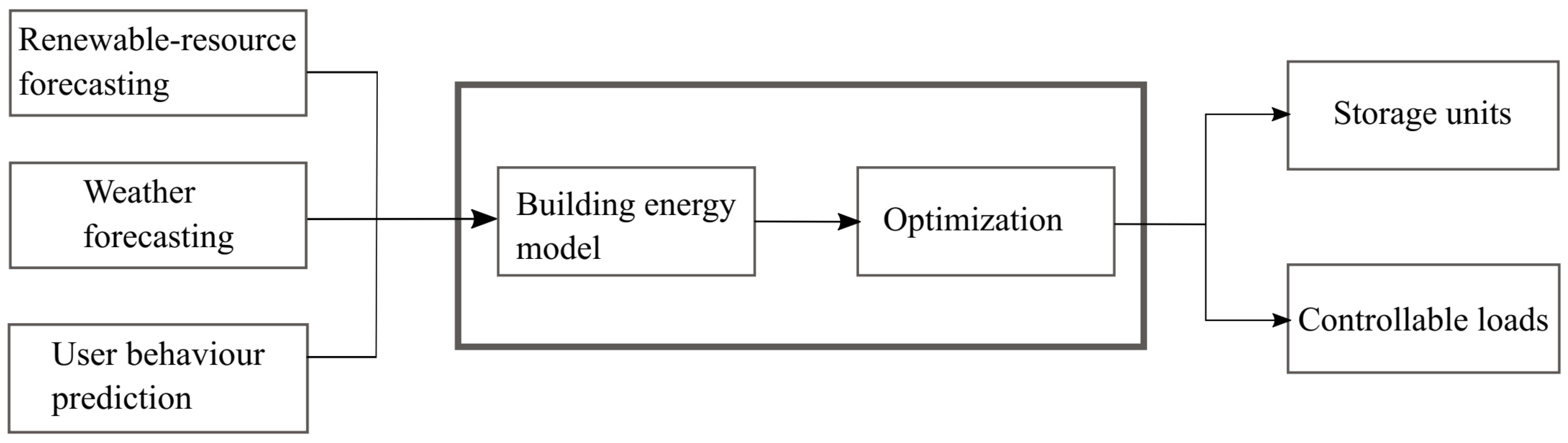
Subsequently, the collected data are analyzed for building monitoring and control, and energy audits. A typical building control schematic—for example, Model predictive control—is shown in Figure 3 below.

In this control scheme, the power flows to and from storage units. Renewable resources and controllable loads are regulated in order to attain multiple objectives: maximize renewable energy utilization, save energy, reduce CO₂ emissions, minimize costs, etc. This scheme requires the building energy model, user behavior model, and weather forecast model to perform its predictive control [27].

• User behavior model: in order to develop the user behavior model, building profile data such as occupancy density, operation schedule, and user interests are essential [6,8,11,28].
• Renewable resource forecast model and weather forecast model: environmental data such as outdoor temperature, outdoor humidity, wind speed, and solar radiation are valuable for developing a wind-speed prediction model, solar radiation prediction model, outdoor temperature prediction model, etc. [29,30].
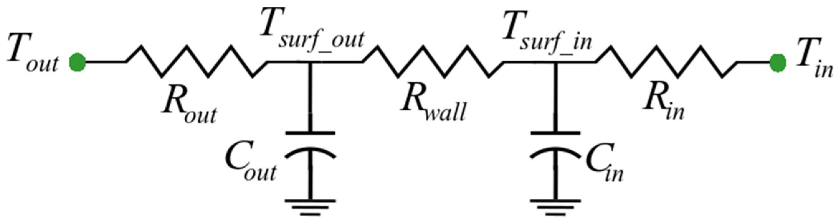
• Building-energy model: The building-energy model includes a PV system model, battery system model, and HVAC model. Electrical data, such as battery state of charge, HVAC power consumption, PV production, etc., are required to update these models’ states. The building model is also an essential component of the building-energy model. Building a thermal model takes into account wall and roof heat transfer, zone air infiltration, and solar radiation impact, where wall heat-transfer can be modeled as 3R2C [11,31,32] as in Figure 4 with $R_{out}$, $R_{in}$, $C_{out}$, $C_{in}$ representing the thermal resistance and thermal storage capacity of the wall and $T_{out}$, $T_{\mathrm{in}}$, $T_{surf\_out}$, $T_{surf\_in}$ being outdoor temperature, indoor temperature, wall-outside-surface temperature and wall-inside-surface temperature, respectively. Data of wall-surface temperatures need to be collected to find the model’s parameters (capacitances and resistances) [11].

The database acquired by the building monitoring system is significant for developing control strategies in smart buildings. That is why sensor maintenance, data quality issues, and data compensation must be taken seriously. However, sensors might work inconsistently for multiple reasons: harsh environments, manufacturing defects, sensor positions (near to metal cabinets, far away from the gateway, etc.), power failure, and Wi-Fi disconnection. 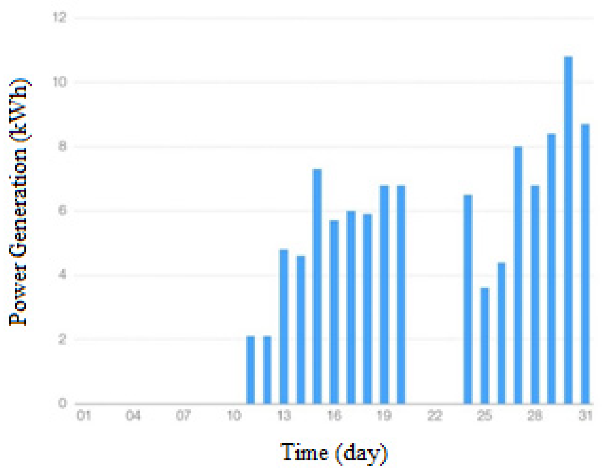Figure 5 gives an example of data loss due to Wi-Fi disconnection in a PV power system. As can be seen in this figure, the data of PV power generation were lost for a number of days in August, 2022.

The diverse datasets can provide a lot of information that allows us to accomplish the task of ensuring the reliability and data recovery of the measuring points in the network. However, more parameters in a model are not ensuring a good model due to a lot of uncertain input parameters [33]. Considering the correlation between input selection and dataset size for the model is still a challenge, as missing data or redundant data can lead to prediction errors.

Research on the detection of inconsistent data and data compensation in smart buildings not only helps us to early identify sensor failures, but also allows us to compensate for the lost and low-quality data, which is essential to improve the building control and management system resilience and reliability.

3. Methodology

3.1. Approach

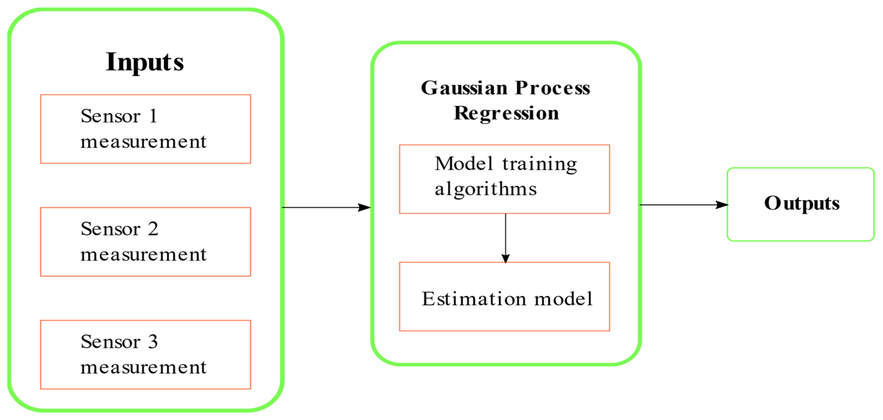
The idea of this paper is to develop a model that can infer the data at a preselected sensor node (the output) in the sensor network from the data at several other sensor nodes (the inputs) in the same network. The model belongs to the class of statistical models or the class of neural network models. This approach is illustrated in Figure 6 below. The input–output selection depends on the correlation degree of these variables. For example, the total power consumption of a building is usually correlated with the indoor and outdoor temperatures and the occupancy of that building. The input–output mapping—the estimation model—is trained by Gaussian process regression. Afterward, the estimation model is used to detect inconsistent data and data loss at the output sensor node by comparing the inference (the estimation) and the actual measurement (observation). The lost data can be compensated by taking the estimation in place.

The input–output pair could be diverse due to the richness of sensor nodes in a building. However, adequate data compensation certainly improves the accuracy of building modeling and building control reliability.

Predicted models detect anomalies and compensated data, but it will be challenging to process a relatively large amount of data simultaneously. The data-driven approach can be time consuming in testing and requires computing capacity, but it is reliable to address in practice. In this work, we will approach GPR with small datasets with a minimized number of input variables to reduce the complication and computing speed.

3.2. Principle of Gaussian Process Regression

Gaussian process regression is a statistical approach that tries to approximate input–output mappings from empirical data using a Gaussian process model [34]. This is used in regression and prediction problems. Suppose that the input–output mapping is expressed by the following function:

$$y=f\left(X\right)=\left[\begin{array}{c}f(x[1])\\ f(x[2])\\ f(x[3])\\ ⋮\\ f(x[n])\end{array}\right]=\left[\begin{array}{c}y[1]\\ y[2]\\ y[3]\\ ⋮\\ y[n]\end{array}\right]$$

(1)

where $x[\mathrm{i}]$ is an input vector at sample $\mathrm{i}$ and $y[\mathrm{i}]$ is the corresponding output. The basic assumption is that the output vector $y=\left[\begin{array}{c}y[1]\\ y[2]\\ y[3]\\ ⋮\\ y[n]\end{array}\right]$ has a multivariate Gaussian distribution. Then, if a subset of $y$ is observed, the distribution of the complementary subset could be derived using the properties of multivariate Gaussian distributions.

A Gaussian Process is formally defined as a collection of random variables, any finite number of which have a joint Gaussian distribution. A Gaussian Process of a real process $y=f\left(X\right)$ is fully specified by the mean function $m\left(X\right)$ and the covariance matrix formed from a covariance function $k\left(x[\mathrm{i}],x[\mathrm{j}]\right)$

$$\begin{array}{l}m\left(X\right)=\mathrm{E}\left[f\left(X\right)\right]\\ k\left(x[\mathrm{i}],x[\mathrm{j}]\right)=\mathrm{cov}\left(f\left(x[\mathrm{i}]\right),f\left(x[\mathrm{j}]\right)\right)\end{array}$$

(2)

where $\mathrm{E}$ denotes the expectation.

In this research, the mean function is initialized at $0$ [34], while the square exponential or Radial Basis Function (RBF) is selected as the covariance function (also called the kernel), since it is infinitely differentiable and is therefore appropriate for modeling the characteristic of smoothness of a function [24]. The RBF kernel is given by [34]:

$$k\left(x[\mathrm{i}],x[\mathrm{j}]\right)=e^{\frac{1}{2l^2}{‖x[\mathrm{i}]-x[\mathrm{j}]‖}^2}$$

(3)

The RBF kernel is based on the idea that the closer the two vectors in input space, the higher the covariance between them. RBF kernel has one hyper-parameter $l$ (called length-scale) to control how the distance in the input space is considered as “close”.

Now, consider two subsets of $y$: $y_1=f\left(X_1\right)$ and $y_2=f\left(X_2\right)$ with $X=\left[\begin{array}{l}{X}_1\\ X_2\end{array}\right]$ such that:

$$y=\left[\begin{array}{l}{y}_1\\ y_2\end{array}\right]~N\left(0,\left[\begin{array}{cc}{\sum }_{11}& {\sum }_{12}\\ {\sum }_{21}& {\sum }_{22}\end{array}\right]\right)$$

(4)

with ${\sum }_{ij}=k\left(X_i,X_j\right)$ being the covariance matrices. The conditional distribution $P\left(y_2|y_1,X_1,X_2\right)$ is multivariate normal:

$$P\left(y_2|y_1,X_1,X_2\right)~N\left({\sum }_{21}{{\sum }_{11}}^{-1}{y}_1,{\sum }_{22}-{\sum }_{21}{{\sum }_{11}}^{-1}{\sum }_{12}\right)$$

(5)

With the mean to be selected as a replacement of $y_1$ in case this output subset is lost.

The Gaussian process model $y=f\left(X\right)$ is fitted to the training set using the maximum log likelihood method to tune the hyper-parameter (s) in the kernel ($l$ in RBF). Finally, it is tested on the test set by using (Equation (5)) to compute the mean and deviation or confidence interval.

4. Experiments and Results

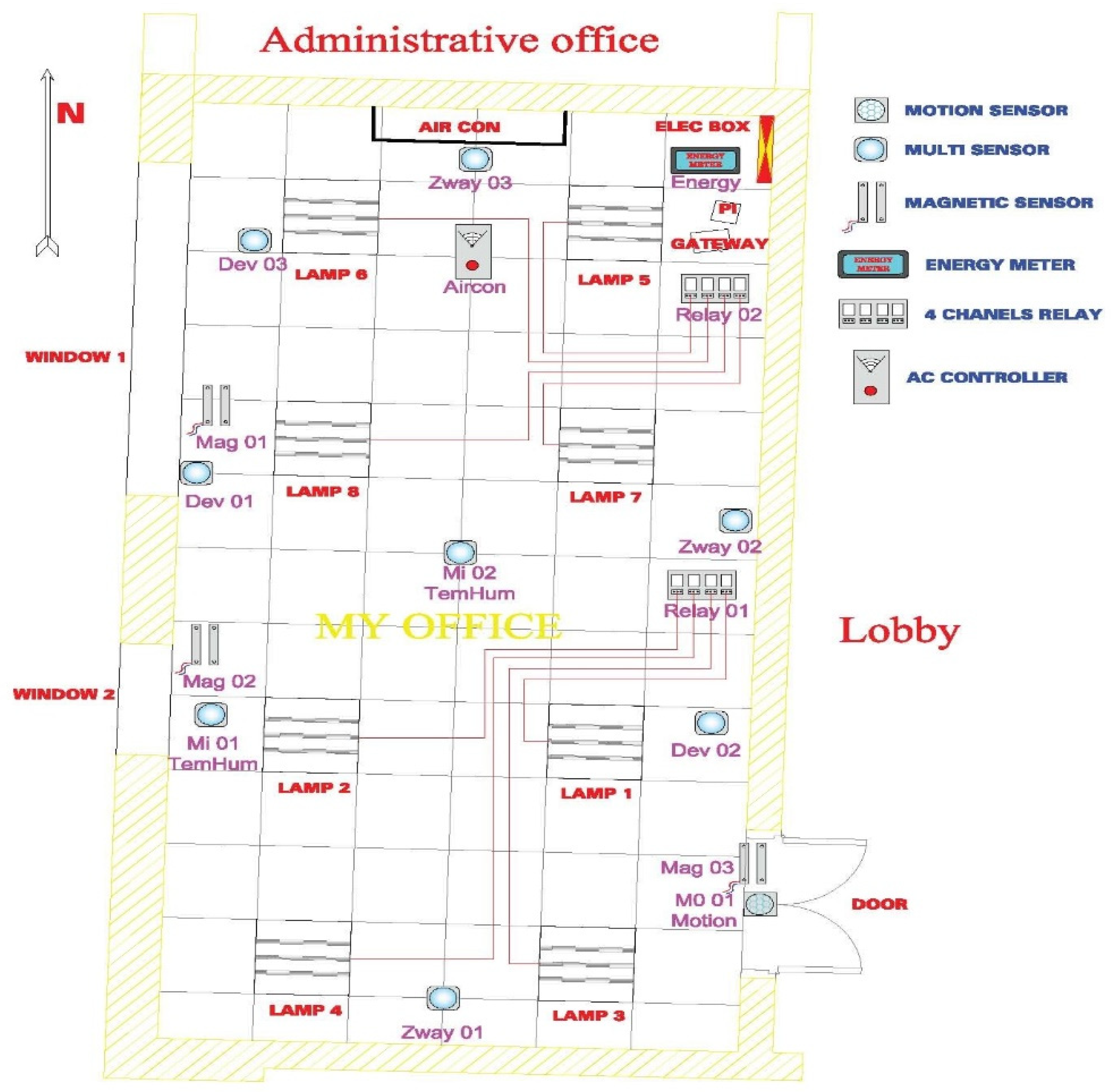
The test case of this research is an office in the Vietnam–Korea Vocational college of Hanoi (VHH). The office was equipped with a low-cost building monitoring platform. Sensor types and locations are shown in Figure 7. There are six multi-sensors (measuring environment parameters) and door sensors/five motion sensors/three energy meters (measuring sub-loads: HVAC, Lighting, and total load power).

Among six multi-sensors, four sensors (Zway01, Zway02, Zway03, and Mi01) are placed on four inner wall surfaces to study the thermal behaviors of the four walls of this building zone. The indoor environment is monitored by Mi02. All the data are collected every 10 min for one year. Although this approach is possibly applicable to different types of input–output pairs of a building’s sensor network, this section presents this research’s application on inconsistent data detection and data compensation for HVAC power, indoor temperature, and PV power.

The objectives of the experiments presented in the following sections are:

-

To use correlations of high-resolution (several minutes) and locally available data (including data from sensor nodes within the building and data from nodes in other buildings within the same area) to develop a predictive model with the goal of data compensation in a sensor network.

-

Considering the fitness of GPR in the predictive models for different types of data nodes (such as power consumption, PV power, and indoor temperature).

-

Evaluate the model’s computational performance for small dataset sizes (weeks and months).

All code is written in Python. The hardware used in all of the following experiments is an Intel Core i7-8550U 1.80 GHz CPU.

4.1. Experiment 1: Detection and Compensation of Inconsistent HVAC Data

This experiment includes two small experiments to evaluate the performance of the proposed method in detecting the appearance of inconsistent data, and compensates for inconsistent data and data loss for HVAC power data. The computation efficiency of the proposed method is considered as well.

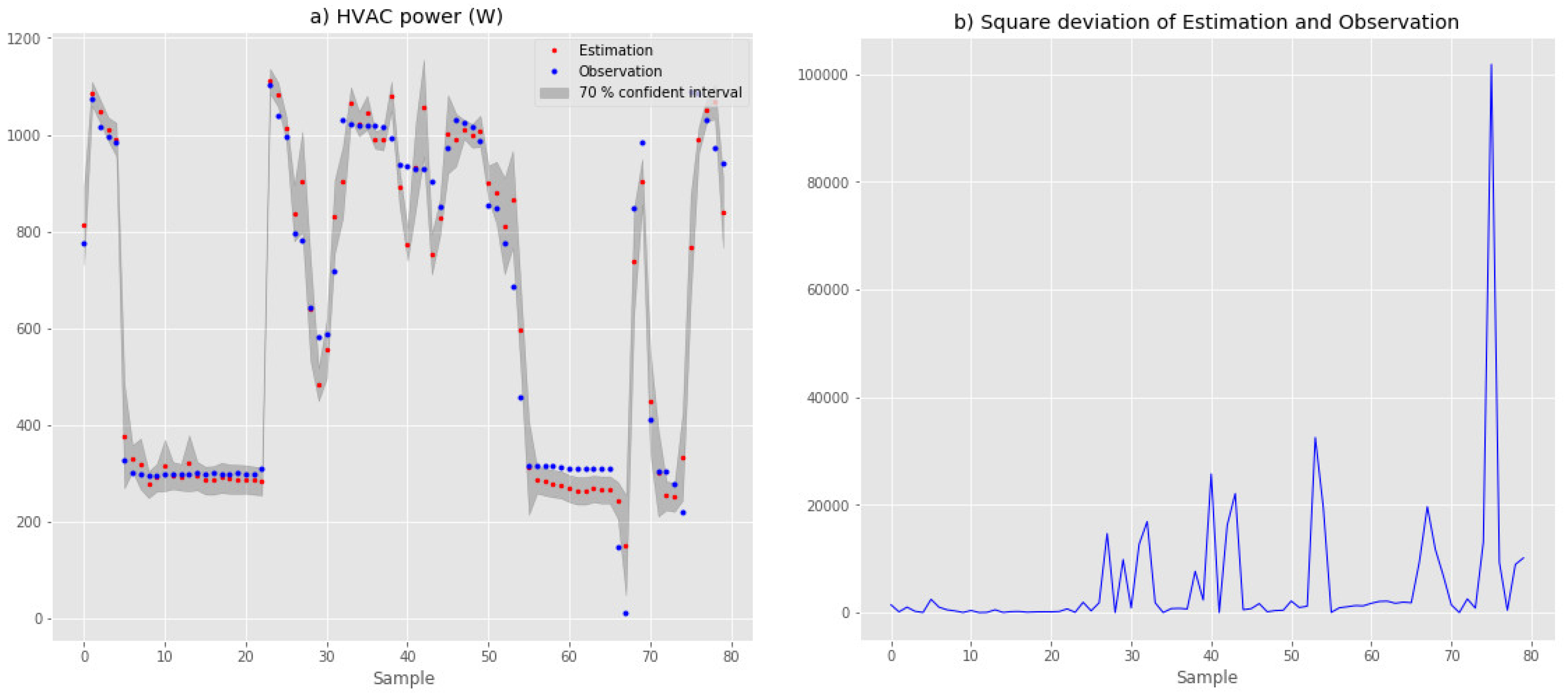
In the experiment detecting inconsistent data, the training dataset was collected in July 2020, while the data for August 2020 were used as the test dataset. The HVAC data in the test dataset are intentionally distorted by a bias of 10 W, since sample 25. The input–output of the model is shown in

Table 1. Input–output pair of Experiment 1.

Inputs	Output
$x[\mathrm{k}]=\left[TiZ3[\mathrm{k}],HVAC[\mathrm{k}-1],\hspace{0.17em}Total\_power[\mathrm{k}]\right]$	$y[\mathrm{k}]=HVAC[\mathrm{k}]=\mathrm{f}(x[\mathrm{k}])$

, where $TiZ3[\mathrm{k}]$ is the temperature at node Zway 03, $HVAC[\mathrm{k}]$ is the HVAC power of the office at time t and $HVAC[\mathrm{k}-1]$ is the previous sample; $Total\_power[\mathrm{k}]$ is the total power consumption of the office, assuming that not all the load powers of the office are measured.

Inconsistent data are detected by comparing the observation in the test dataset to the output inference of the trained model (the estimation). Figure 8a below displays the estimation and observation with the boundaries of a 70% confidence interval to be an indication of the observation’s uncertainty. It can be seen that, after sample 25, there are a number of observations (blue points) outside the confidence interval. In Figure 8b, the square deviation of the estimation and observation is shown. As a result, the error increases significantly after sample 25, signaling the moment at which the inconsistency in the HVAC power data appears. This kind of fault detection provides a great benefit to the building operators for monitoring the sensor network’s operation, sensor calibration and maintenance.

In the experiment of HVAC data compensation, the proposed method’s ability to compensate HVAC power inconsistent data and data loss and its computation efficiency are considered.

The input–output pair is shown in

Table 2. Input–output pair of Experiment 1.

Inputs	Output
$x[\mathrm{k}]=\left[TiZ3[\mathrm{k}],outTemp[\mathrm{k}],\hspace{0.17em}Total\_power[\mathrm{k}]\right]$	$y[\mathrm{k}]=HVAC[\mathrm{k}]=\mathrm{f}(x[\mathrm{k}])$

, where $TiZ3[\mathrm{k}]$ is the temperature at node Zway03, $outTemp[\mathrm{k}]$ is the outdoor temperature collected from a web service, and $Total\_power[\mathrm{k}]$ is the total power consumption of the office.

The dataset was collected in July and August 2020. Different dataset lengths, including one week, two weeks, four weeks, and eight weeks, are selected to evaluate the performance of the proposed method with different small datasets. The test dataset is taken randomly with a ratio of 50%, except for the 8-week dataset, for which the training dataset is the data for the first four weeks (in July) and the test dataset is the remaining data (in August), in order to assess the proposed method’s capability in compensating data loss for a continuous period of time.

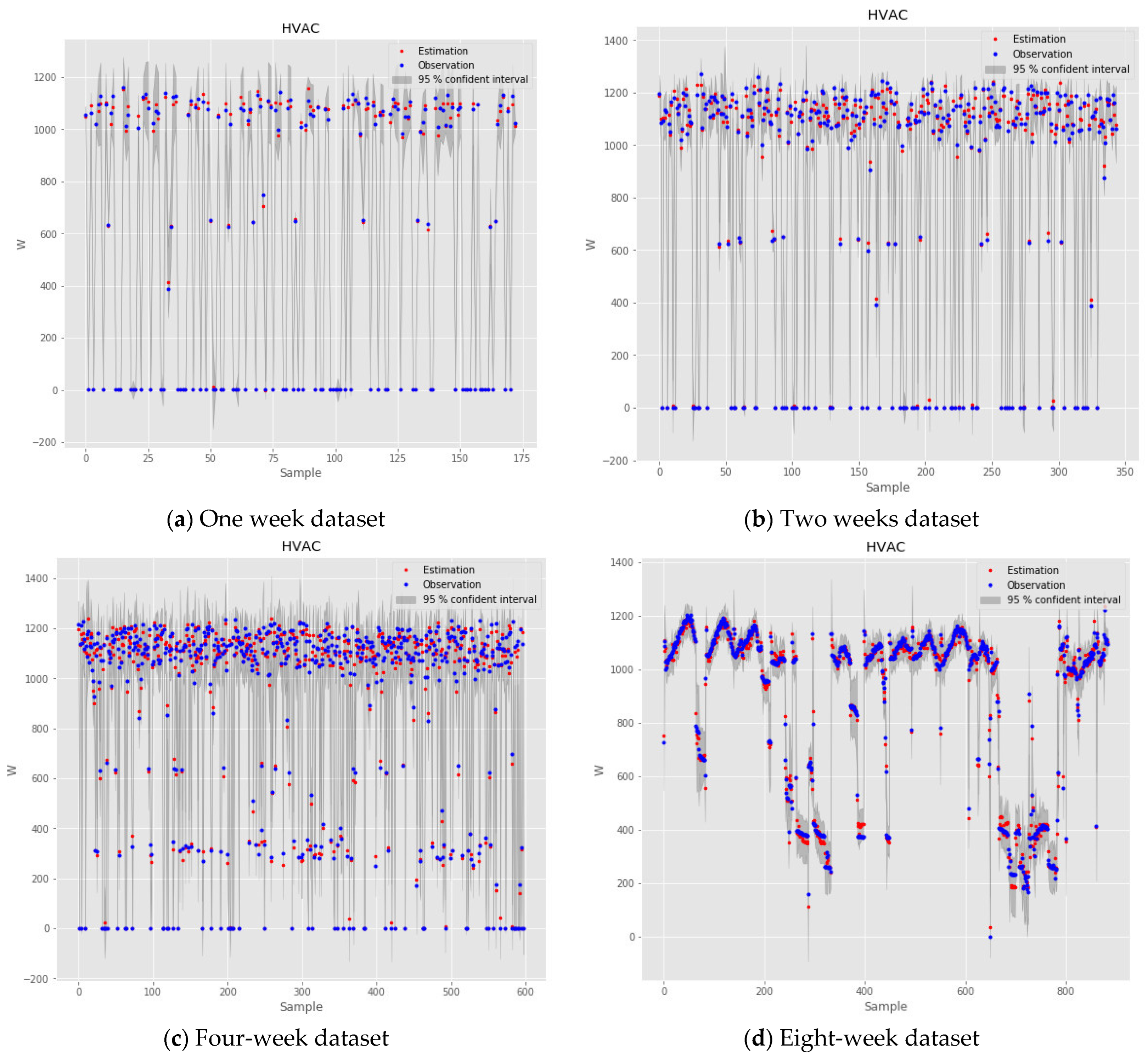
The data compensation results are illustrated in Figure 9a–c, and d below for the dataset length of one week, two weeks, four weeks, and eight weeks, respectively. It can be seen in Figure 9a–c that with data loss at random moments, the estimation closely follows the observation.

However, it is different in Figure 9d when the proposed method compensates for the continuous data loss in a month. The deviation of the estimation and the observation, and the computation of the proposed method for the different dataset lengths are quantified in

Table 3. Performance indices of the compensation of HVAC data.

Dataset Training Dataset (50%)		1 Week	2 Weeks	4 Weeks	8 Weeks
HVAC	Root Mean Square Error (W)	18.21	20.47	23.8	20.5
	Maximum Absolute Error (W)	45.97	48.65	50.9	51.7
	Traning Time (second)	4.4	49	154.4	930

, in which the root mean square errors are around 20 W and the highest maximum absolute error is 51.7 W, which are small numbers regarding the HVAC power range of 1200 W. The training times vary from 4.4 s to 15.5 min as the dataset length increases from 1 week to 8 weeks.

4.2. Experiment 2: Compensation of Lost Temperature Data

As explained in Section 2, temperatures are important data for building thermal modeling, user comfort monitoring, as well as real-time building control. This experiment illustrates the proposed method’s ability to compensate for the indoor temperature data.

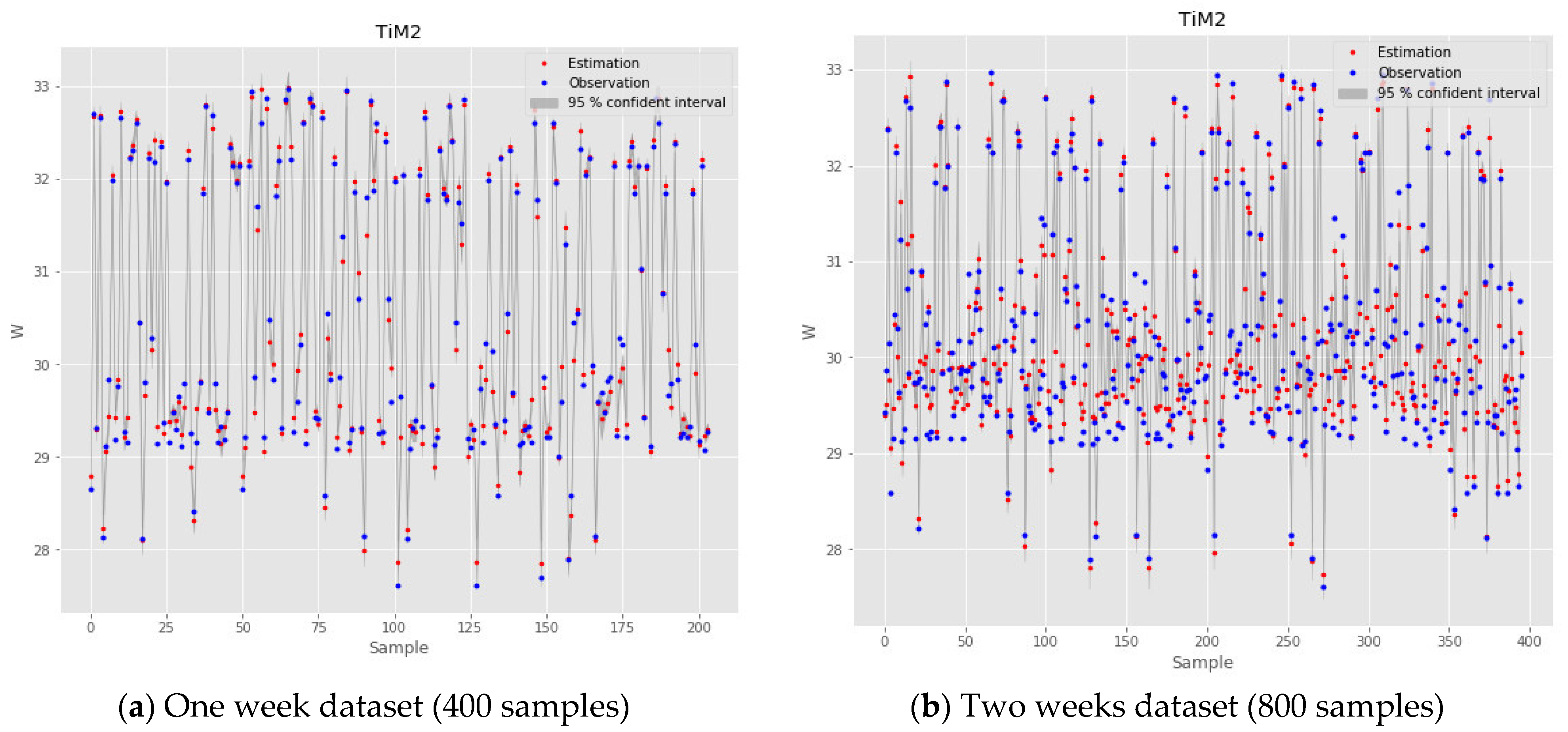
The same four datasets with different lengths of one week, two weeks, four weeks, and eight weeks are selected, as in Experiment 1. The input–output pair is shown in

Table 4. Input–output pair of Experiment 2.

Inputs	Output
$x[\mathrm{k}]=\left[TiZ1[\mathrm{k}],\hspace{0.17em}TiZ2[\mathrm{k}]\right]$	$y[\mathrm{k}]=TiM2[\mathrm{k}]=\mathrm{f}(x[\mathrm{k}])$

below, where $TiM2$ is the indoor temperature at sensor node Mi02, while $TiZ1$ and $TiZ2$ are wall-surface temperatures at nodes $TiZ1$, $TiZ2$ in the office room correspondingly within the office room.

The estimation of the indoor temperature $TiM2$ is compared to the observed (measured) data in the test set, as in Figure 10a–d, for the different dataset lengths, and the quantitative comparison is demonstrated in

Table 5. Performance indices of the compensation of TiM2 data.

Dataset Training Dataset (50%)		1 Week	2 Weeks	4 Weeks	8 Weeks
TiM2	Root Mean Square Error (°C)	0.17	0.22	0.2	0.32
	Maximum Absolute Error (°C)	0.48	0.5	0.46	0.6
	Traning Time (second)	3.25	19	95.5	438

. It is noticeable in these figures that for both data loss at random moments and continuous one-month data loss, the estimation can tightly track the observation.

According to Table 5, the highest root means the square error is 0.32 °C, and the highest maximum absolute errors are from 0.46 °C to 0.6 °C, which is acceptable considering that the highest indoor temperature TiM2 is more than 33 °C. The training times of this experiment varied from 3.25 s to 8 min for the dataset length changing from 1 week to 8 weeks.

4.3. Experiment 3: Compensation of Photovoltaic (PV) Power Data

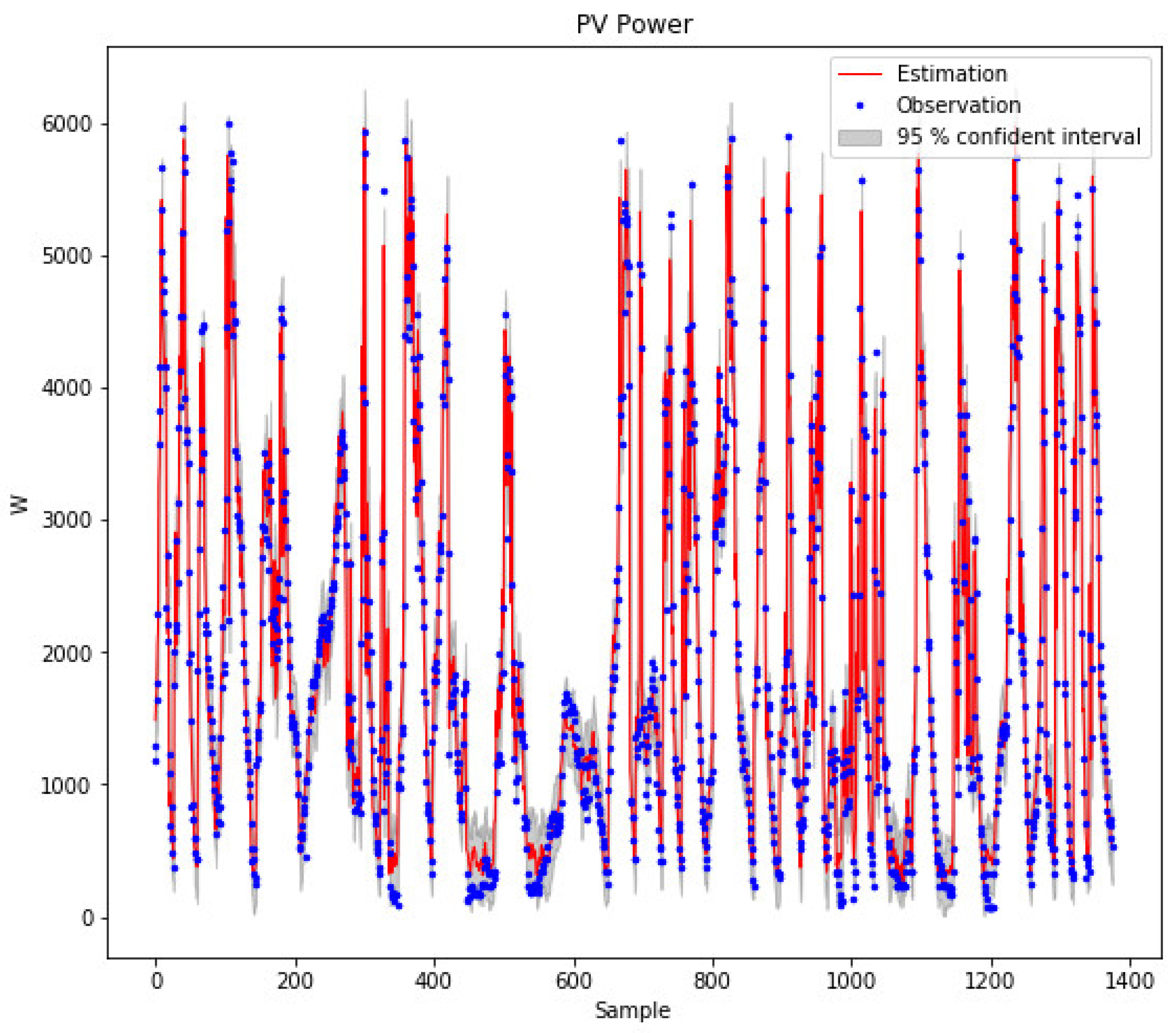
The proposed method is applied in this experiment to compensate for PV power data. The data loss for one PV system is compensated with the available data for the other three PV systems in the same area. The input–output pair is shown in

Table 6. Input–output pair of Experiment 3.

Inputs	Output
$x[\mathrm{k}]=\left[PV1[\mathrm{k}],PV2[\mathrm{k}],\hspace{0.17em}PV3[\mathrm{k}]\right]$	$y[\mathrm{k}]=PV[\mathrm{k}]=\mathrm{f}(x[\mathrm{k}])$

below, where PV [k] is the PV power at the PV system to compensate and PV1 [k], PV2 [k], and PV3 [k] are the available PV powers for the other three PV systems in the local area. The training dataset was collected in July 2022, and the test dataset was acquired in August 2022.

The compensation results are demonstrated in Figure 11 below. In the figure, the estimation goes up and down with the observation, as PV power goes up and then goes down within one day.

The compensation’s performance is detailed in

Table 7. Performance indices of the compensation of PV power data.

PV Power	Root Mean Square Error (W)	Mean Absolute Error (W)	Maximum Absolute Error (W)
	209.6	171.5	429.3

. The root mean square error is 209.6 W, and the mean absolute error is 171.5 W—around 3% and 2.8%, respectively, of the PV system’s maximum power. Meanwhile, the maximum absolute error is 429.3 W, representing 7% of the maximum power. These measured indices are pleasant, although they can be improved when the distances between these PV systems become smaller.

5. Discussions

In Experiment 1, data gaps in the HVAC power due to a failure power meter were filled by Gaussian-process-associated confidence intervals.

Figure 9 shows that the computational time requirement of GPR increases rapidly as the training dataset sizing decreases. In Table 3, the root mean square error was used to evaluate the fitting quality of the Gaussian process regression over different time periods. The goodness of fit can also be assessed by interpreting the 95% confidence interval on the regression points. This approach introduces average error and a local assessment of GPR on the short data.

The results show that the GPR approach provides good prediction and compensation results for HVAC, room temperature, and PV power data with datasets under one month. In addition, the correlation of the data can improve model quality.

Weather data are used in many studies to forecast PV output and HVAC consumption. However, high-resolution weather data (minute by minute) are unavailable in the local area. Experiments 1 and 3 show that it is possible to compensate by correlating local data, such as the indoor temperature for HVAC consumption forecasting, or using data from PV power measurement nodes in neighboring stations for capacity forecasting PV.

In Experiment 2, the high spatially dense distribution of room-temperature sensor nodes allows data compensation and the development of a virtual temperature sensor with high accuracy.

We calculate the average time required for the trained models at a query data point. The computation time of GPR is significantly lower with the small dataset, at one week, two weeks, or four weeks (a rounding of 200, 400, and 800 samples) but ensures prediction accuracy.

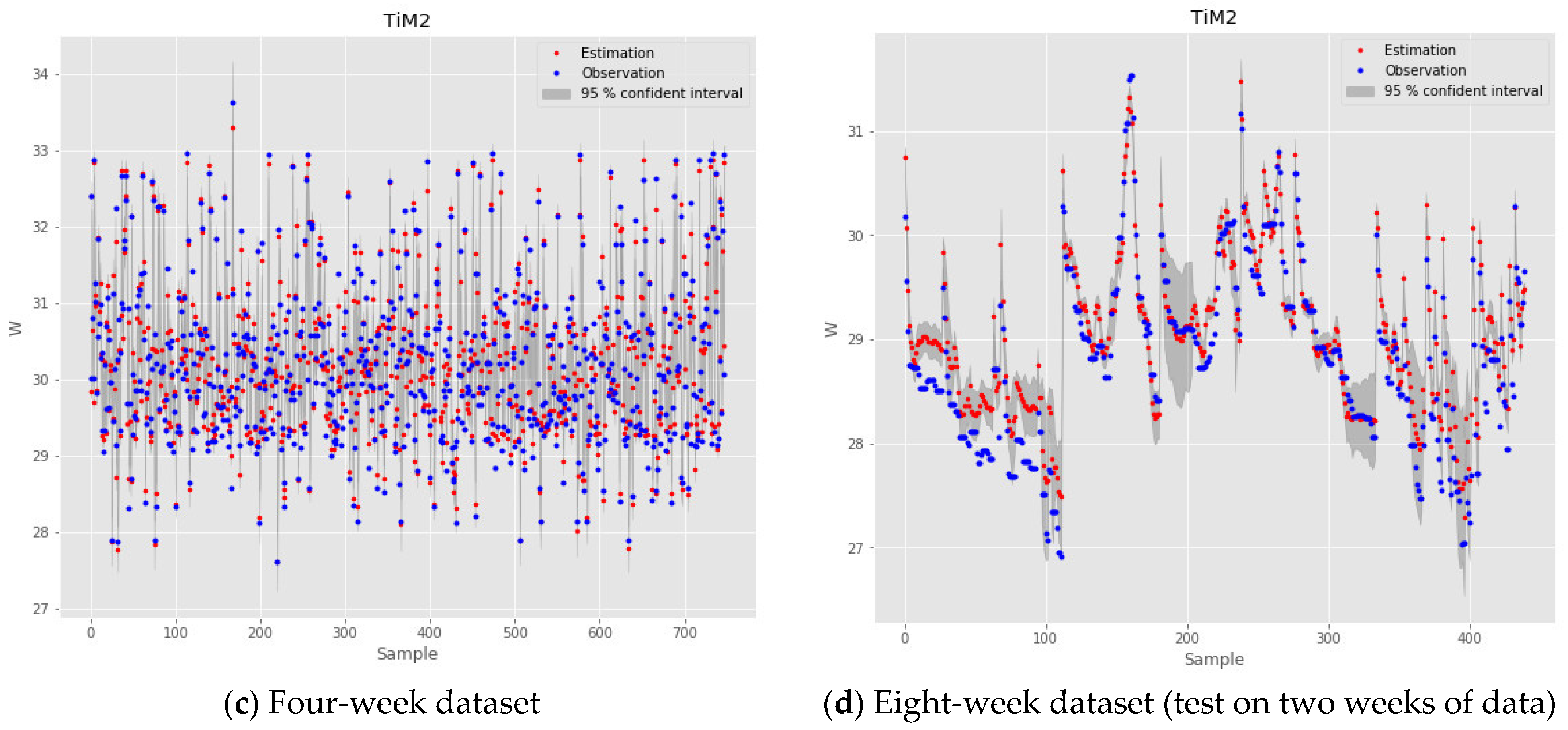
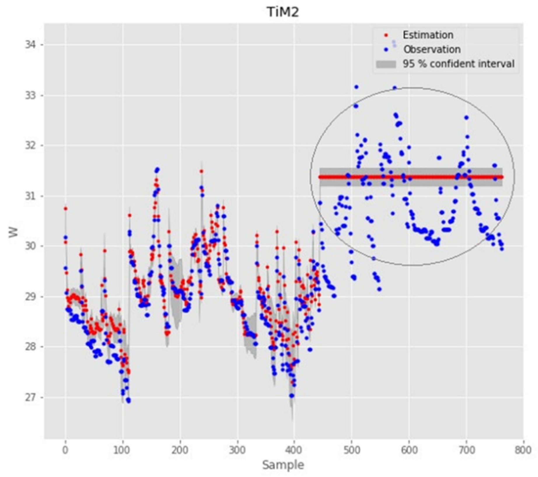
Particularly in Experiment 2, we note the room-temperature data at the TiM2 sensor location for eight weeks with the train-set ratio 50–50. Figure 12 below shows the data compensation for August using the model trained with these data in July. In this figure, there is a significant compensation error on the test data of the last two weeks of the month, which is of a higher temperature range. To explain, it may be the difference in data features in months, such as weather and user activity in the two months. This explanation is also consistent with previous studies. For example, a study in [21] shows the importance of input features in predictive models. The data structure combines the fluctuation components such as weather by seasons and human activities by the time [25,26], which could give a more robust model. Therefore, adding the correlation variables to the model and more data for model training may need to be considered. However, this can increase the model’s complexity and computation time.

Splitting to the sub-datasets for GPR models will speed up the model computation while ensuring prediction results. Furthermore, the length of the dataset in this experiment is about 200 samples for the training model, and the computation speed is less than 5 s, which is quite suitable for the online model.

The computing speed depends on the configuration of different computers. However, choosing standard configurations of computers in offices can allow us to conclude the model’s complexity (including the number of involved variables and the length of the dataset available for the model) and calculation cost.

6. Conclusions

Applications in smart buildings always require a monitoring system with a large number of sensor nodes. The monitoring system is responsible for establishing a database that, in turn, serves optimal energy control and management while guaranteeing human comfort. Sensor operation and maintenance and data quality monitoring are essential but challenging tasks.

This paper developed a data-analysis method based on Gaussian process regression to analyze data for detecting and compensating for inconsistent data and data loss due to sensor imperfections. The experiments implemented in the VHH building in this research prove the proposed method’s efficiency at detecting HVAC-inconsistent data and compensating data of HVAC power, indoor temperature, and PV power. The research results demonstrate that the method presented in this paper applies to different data types in building energy management.

This paper also confirms the computation efficiency of the proposed method and its fitness in building online control tasks. The proposed method effectively solves the problem of sensor operation and maintenance. Its ability to improve data quality supports the control system in smart buildings. This research is a stepping stone for further research on online monitoring and control systems in larger-scale smart buildings in particular, and smart grids in general.

References

- United Nations Environment Programme and Global Alliance for Buildings and Construction. 2020 Global Status Report for Buildings and Construction: Towards a Zero-emissions, Efficient and Resilient Buildings and Construction Sector—Executive Summary. 2020. Available online: https://wedocs.unep.org/xmlui/handle/20.500.11822/34572 (accessed on 26 September 2022).
- Wurtz, F.; Delinchant, B. “Smart buildings” integrated in “smart grids”: A key challenge for the energy transition by using physical models and optimization with a “human-in-the-loop” approach. Comptes Rendus. Phys. 2017, 18, 428–444. [Google Scholar] [CrossRef]
- Delinchant, B.; Dang, H.A.; Vu, H.T.T.; Nguyen, D.Q. Massive arrival of low-cost and low-consuming sensors in buildings: Towards new building energy services. IOP Conf. Ser. Earth Environ. Sci. 2019, 307, 012006. [Google Scholar] [CrossRef]
- Bae, Y.; Bhattacharya, S.; Cui, B.; Lee, S.; Li, Y.; Zhang, L.; Im, P.; Adetola, V.; Vrabie, D.; Leach, M.; et al. Sensor impacts on building and HVAC controls: A critical review for building energy performance. Adv. Appl. Energy 2021, 4, 100068. [Google Scholar] [CrossRef]
- Rashid, A.; Pecorella, T.; Chiti, F. Toward Resilient Wireless Sensor Networks: A Virtualized Perspective. Sensors 2020, 20, 3902. [Google Scholar] [CrossRef]
- Yuan, J.; Zhou, Z.; Tang, H.; Wang, C.; Lu, S.; Han, Z.; Zhang, J.; Sheng, Y. Identification heat user behavior for improving the accuracy of heating load prediction model based on wireless on-off control system. Energy 2020, 199, 117454. [Google Scholar] [CrossRef]
- Ullah, I.; Ahmad, R.; Kim, D. A Prediction Mechanism of Energy Consumption in Residential Buildings Using Hidden Markov Model. Energies 2018, 11, 358. [Google Scholar] [CrossRef]
- Paone, A.; Bacher, J.-P. The Impact of Building Occupant Behavior on Energy Efficiency and Methods to Influence It: A Review of the State of the Art. Energies 2018, 11, 953. [Google Scholar] [CrossRef]
- Hou, J.; Li, H.; Nord, N.; Huang, G. Model predictive control under weather forecast uncertainty for HVAC systems in university buildings. Energy Build. 2022, 257, 111793. [Google Scholar] [CrossRef]
- Behrooz, F.; Mariun, N.; Marhaban, M.H.; Radzi, M.A.M.; Ramli, A.R. Review of Control Techniques for HVAC Systems—Nonlinearity Approaches Based on Fuzzy Cognitive Maps. Energies 2018, 11, 495. [Google Scholar] [CrossRef]
- Dong, B.; Lam, K.P. A real-time model predictive control for building heating and cooling systems based on the occupancy behavior pattern detection and local weather forecasting. Build. Simul. 2014, 7, 89–106. [Google Scholar] [CrossRef]
- Zaidan, M.A.; Motlagh, N.H.; Fung, P.L.; Lu, D.; Timonen, H.; Kuula, J.; Niemi, J.V.; Tarkoma, S.; Petaja, T.; Kulmala, M.; et al. Intelligent Calibration and Virtual Sensing for Integrated Low-Cost Air Quality Sensors. IEEE Sens. J. 2020, 20, 13638–13652. [Google Scholar] [CrossRef]
- Park, D.; Yoo, G.-W.; Park, S.-H.; Lee, J.-H. Assessment and Calibration of a Low-Cost PM2.5 Sensor Using Machine Learning (HybridLSTM Neural Network): Feasibility Study to Build an Air Quality Monitoring System. Atmosphere 2021, 12, 1306. [Google Scholar] [CrossRef]
- Liang, L. Calibrating low-cost sensors for ambient air monitoring: Techniques, trends, and challenges. Environ. Res. 2021, 197, 111163. [Google Scholar] [CrossRef]
- Cheng, Y.; Li, X.; Li, Z.; Jiang, S.; Jiang, X. Fine-Grained Air Quality Monitoring Based on Gaussian Process Regression. In Neural Information Processing; Springer: Cham, Switzerland, 2014; pp. 126–134. [Google Scholar] [CrossRef]
- Lilley, M.; Frean, M. Neural Networks: A Replacement for Gaussian Processes? In Intelligent Data Engineering and Automated Learning—IDEAL 2005; Springer: Berlin/Heidelberg, Germany, 2005; pp. 195–202. [Google Scholar] [CrossRef]
- Matschek, J.; Gonschorek, T.; Hanses, M.; Elkmann, N.; Ortmeier, F.; Findeisen, R. Learning References with Gaussian Processes in Model Predictive Control applied to Robot Assisted Surgery. In Proceedings of the 2020 European Control Conference (ECC), Saint Petersburg, Russia, 12–15 May 2020; pp. 362–367. [Google Scholar] [CrossRef]
- Matschek, J.; Findeisen, R. Learning supported Model Predictive Control for Tracking of Periodic References. In Proceedings of the 2nd Conference on Learning for Dynamics and Control, Berkeley, CA, USA, 11–12 June 2020; pp. 511–520. Available online: https://proceedings.mlr.press/v120/matschek20a.html (accessed on 20 November 2022).
- Matschek, J.; Himmel, A.; Sundmacher, K.; Findeisen, R. Constrained Gaussian Process Learning for Model Predictive Control. IFAC-PapersOnLine 2020, 53, 971–976. [Google Scholar] [CrossRef]
- Ostafew, C.J.; Schoellig, A.P.; Barfoot, T.D.; Collier, J. Learning-based Nonlinear Model Predictive Control to Improve Vision-based Mobile Robot Path Tracking. J. Field Robot. 2016, 33, 133–152. [Google Scholar] [CrossRef]
- Delinchant, B.; Martin, G.; Laranjeira, T.; Vu, T.-T.-H.; Shahid, M.S.; Wurtz, F. Machine Learning on Buildings Data for Future Energy Community Services. In Proceedings of the SGE 2021—Symposium de Génie Electrique, Nantes, France, 6–8 July 2021; Available online: https://hal.archives-ouvertes.fr/hal-03638394 (accessed on 20 November 2022).
- Shen, Y.; Seeger, M.; Ng, A. Fast Gaussian Process Regression using KD-Trees. In Advances in Neural Information Processing Systems; MIT Press: Cambridge, MA, USA, 2005; Volume 18, Available online: https://papers.nips.cc/paper/2005/hash/6775a0635c302542da2c32aa19d86be0-Abstract.html (accessed on 20 November 2022).
- Approximation of Gaussian Process Regression Models after Training. Available online: https://www.researchgate.net/publication/221165508_Approximation_of_Gaussian_Process_Regression_Models_after_Training (accessed on 20 November 2022).
- Lubbe, F.; Maritz, J.; Harms, T. Evaluating the Potential of Gaussian Process Regression for Solar Radiation Forecasting: A Case Study. Energies 2020, 13, 5509. [Google Scholar] [CrossRef]
- Tolba, H.; Dkhili, N.; Nou, J.; Eynard, J.; Thil, S.; Grieu, S. Multi-Horizon Forecasting of Global Horizontal Irradiance Using Online Gaussian Process Regression: A Kernel Study. Energies 2020, 13, 4184. [Google Scholar] [CrossRef]
- Vu, T.T.H.; Delinchant, B.; Phan, A.T.; Bui, V.C.; Nguyen, D.Q. A Practical Approach to Launch the Low-Cost Monitoring Platforms for Nearly Net-Zero Energy Buildings in Vietnam. Energies 2022, 15, 4924. [Google Scholar] [CrossRef]
- Bordons, C.; Garcia-Torres, F.; Ridao, M.A. Model Predictive Control of Microgrids; Springer: Cham, Switzerland, 2020. [Google Scholar]
- Jia, M.; Srinivasan, R.S. Occupant behavior modeling for smart buildings: A critical review of data acquisition technologies and modeling methodologies. In Proceedings of the 2015 Winter Simulation Conference (WSC), Huntington Beach, CA, USA, 6–9 December 2015; pp. 3345–3355. [Google Scholar] [CrossRef]
- Notton, G.; Faggianelli, G.A.; Voyant, C.; Ouedraogo, S.; Pigelet, G.; Duchaud, J.-L. Solar Radiation Forecasting for Smart Building Applications. In Computational Intelligence Techniques for Green Smart Cities; Lahby, M., Al-Fuqaha, A., Maleh, Y., Eds.; Springer International Publishing: Cham, Switzerland, 2022; pp. 229–247. [Google Scholar] [CrossRef]
- Das, U.K.; Tey, K.S.; Seyedmahmoudian, M.; Mekhilef, S.; Idris, M.Y.I.; Van Deventer, W.; Horan, B.; Stojcevski, A. Forecasting of photovoltaic power generation and model optimization: A review. Renew. Sustain. Energy Rev. 2018, 81, 912–928. [Google Scholar] [CrossRef]
- Boodi, A.; Beddiar, K.; Amirat, Y.; Benbouzid, M. Simplified Building Thermal Model Development and Parameters Evaluation Using a Stochastic Approach. Energies 2020, 13, 2899. [Google Scholar] [CrossRef]
- Boodi, A.; Beddiar, K.; Amirat, Y.; Benbouzid, M. Building Thermal-Network Models: A Comparative Analysis, Recommendations, and Perspectives. Energies 2022, 15, 1328. [Google Scholar] [CrossRef]
- Dinh, V.B. Méthodes et Outils pour le Dimensionnement des Bâtiments et des Systèmes Énergétiques en Phase D’esquisse Intégrant la Gestion Optimale. Ph.D. Thesis, Université Grenoble Alpes, Grenoble, France, 2016. Available online: https://tel.archives-ouvertes.fr/tel-01529763 (accessed on 20 November 2022).
- Rasmussen, C.E.; Williams, C.K.I. Gaussian Processes for Machine Learning; MIT Press: Cambridge, MA, USA, 2005. [Google Scholar] [CrossRef]