
Proposal of a System to Identify Failures and Evaluate the Efficiency of Internal Combustion Engines of Thermal Power Plants


 ,
, 
 ,
,  ,
,
Abstract
1. Introduction
2. Materials and Methods
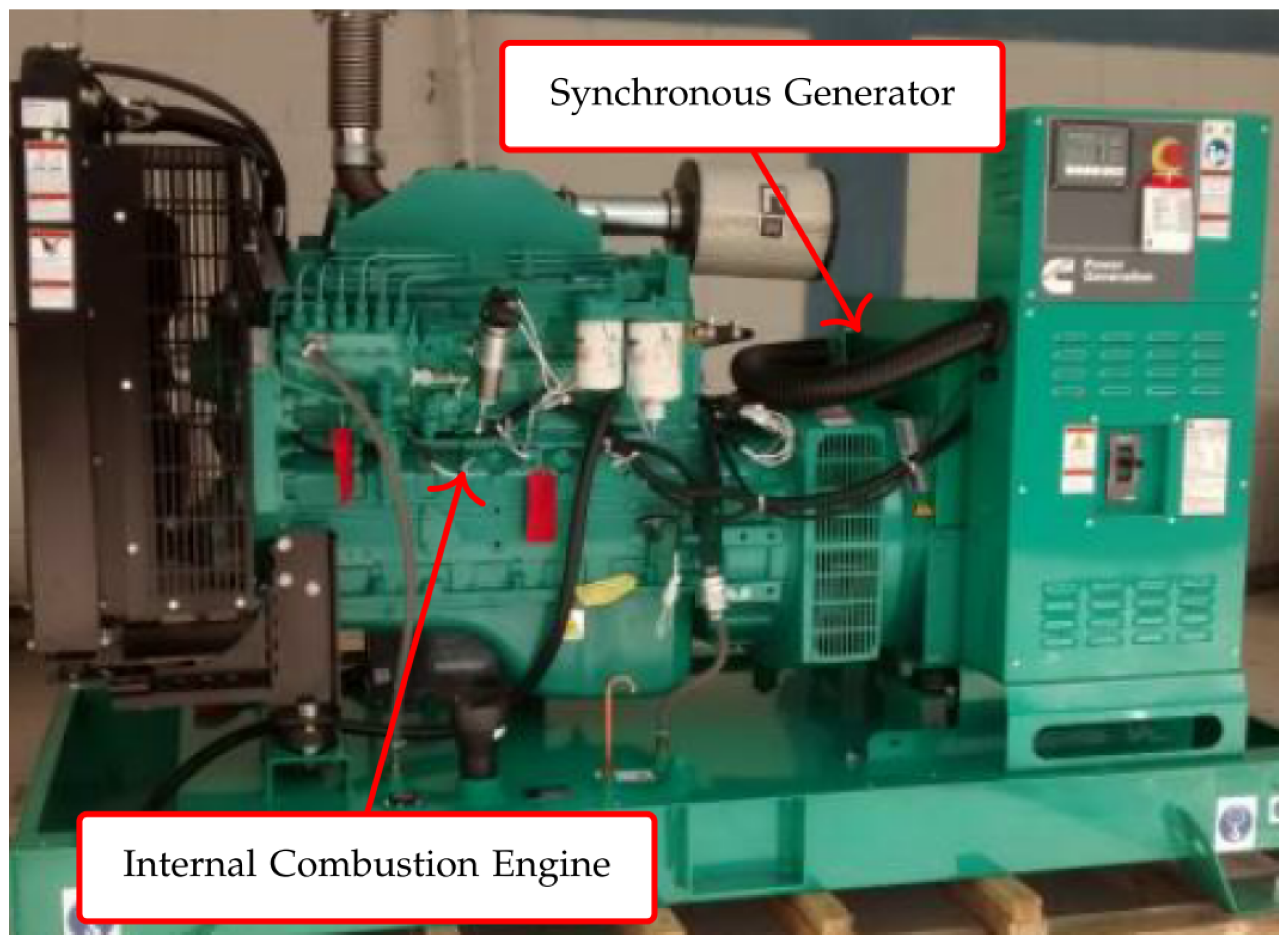
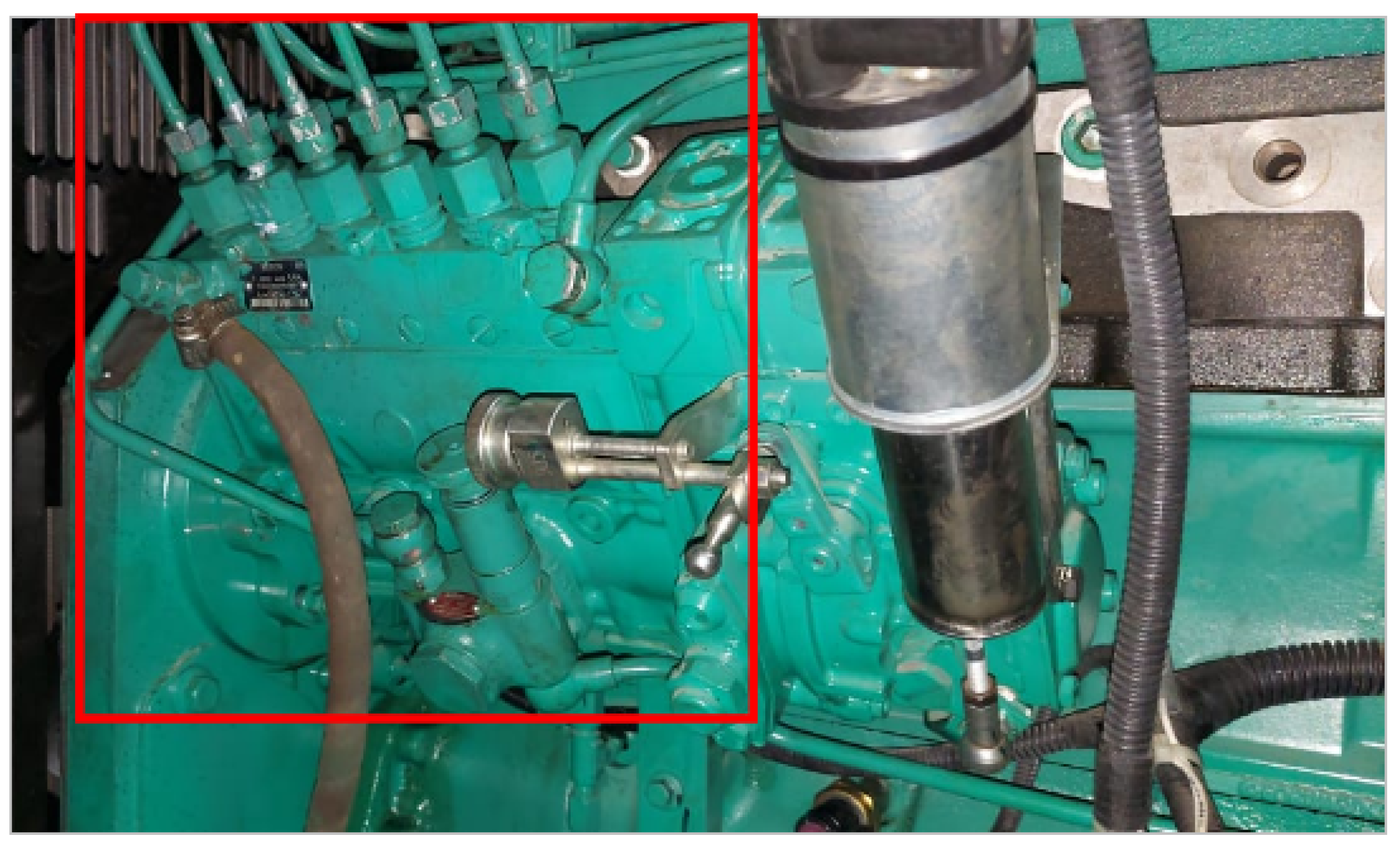
2.1. Internal Combustion Engine Subsystems
- Injection system
- Lubrification system
- Cooling system
- Turbocharger system
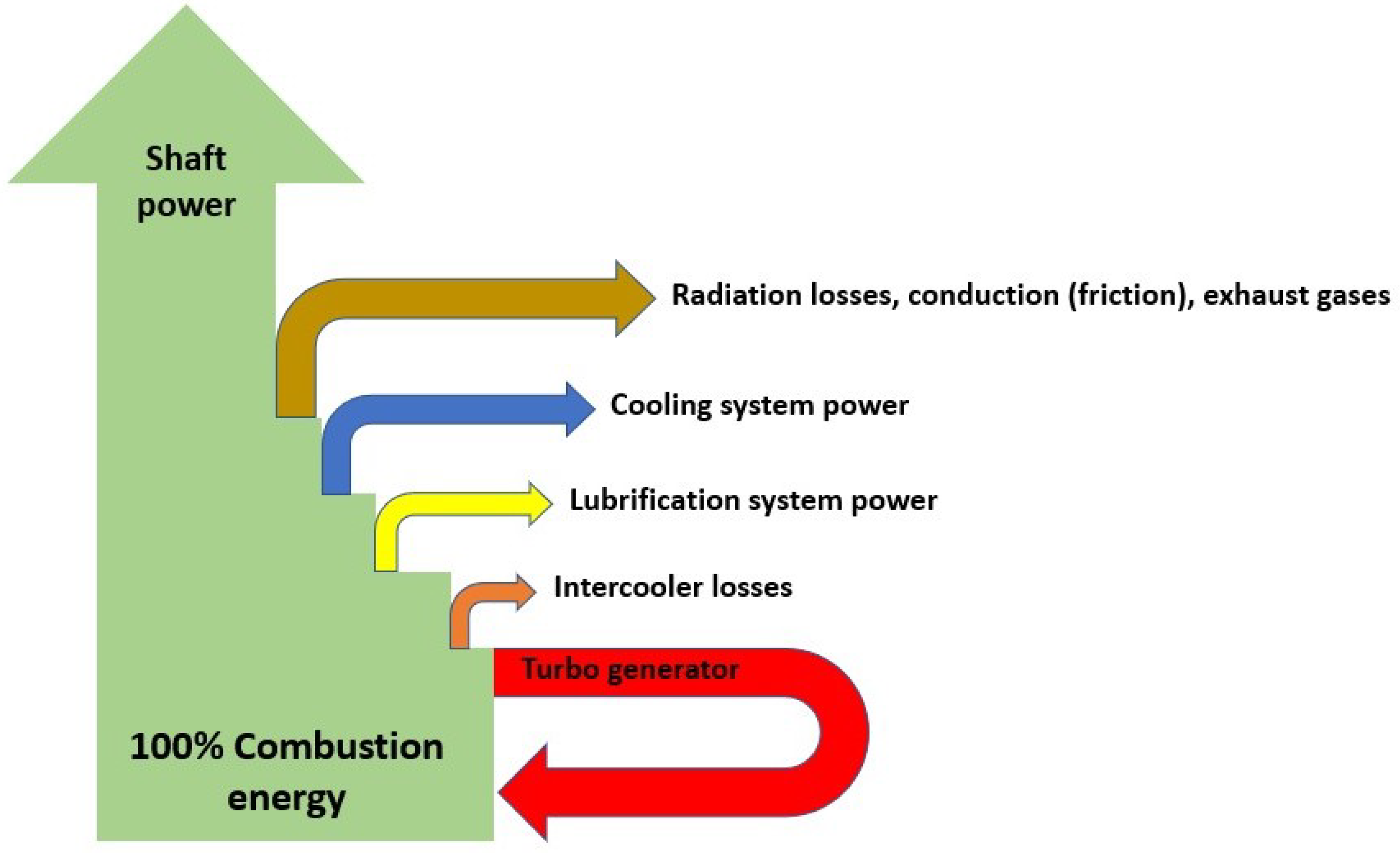
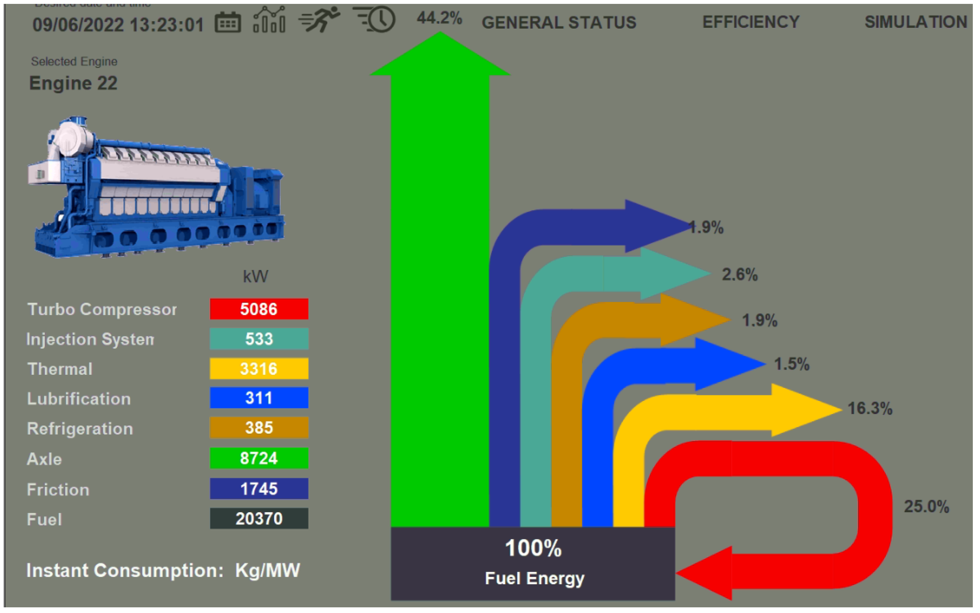
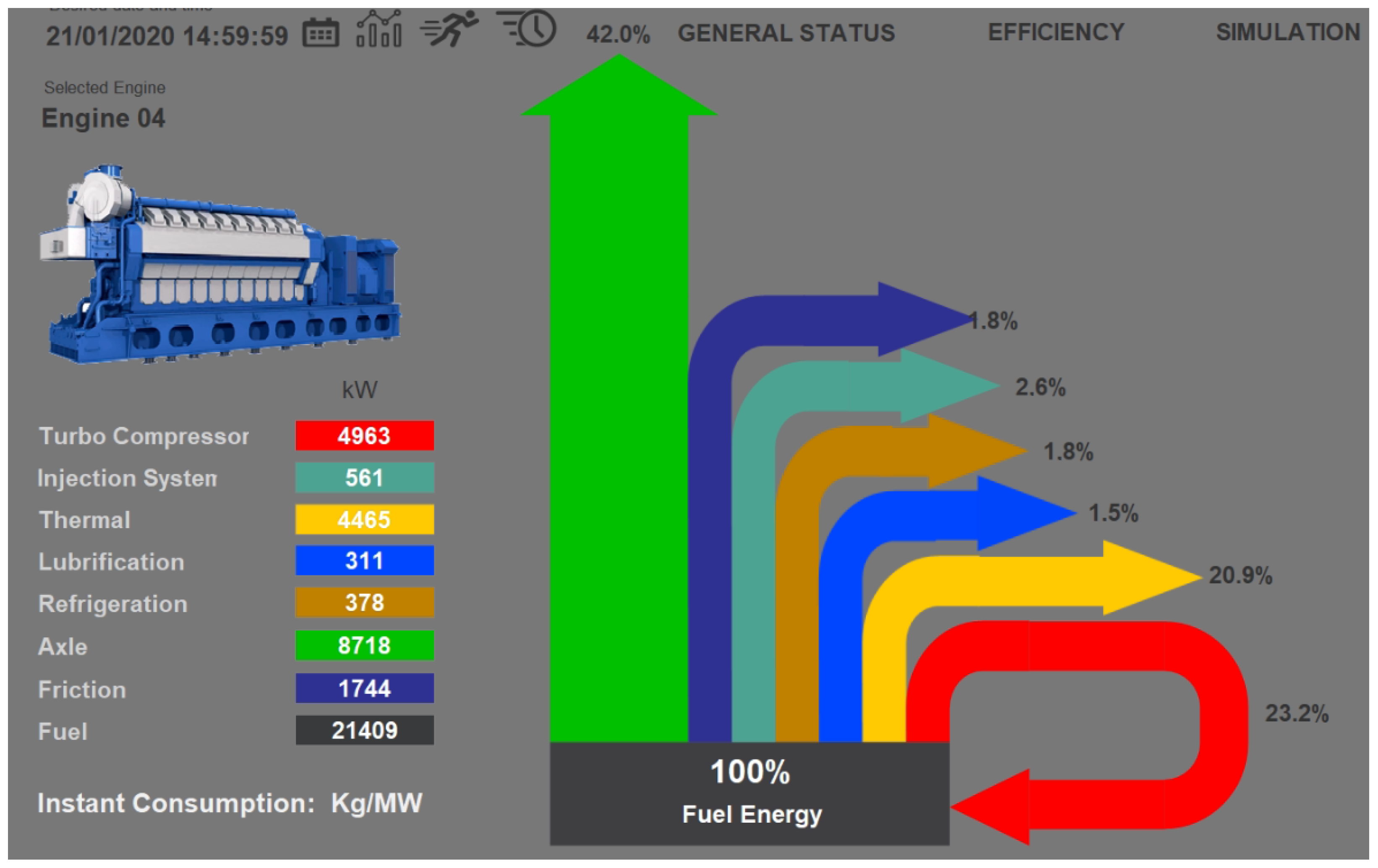
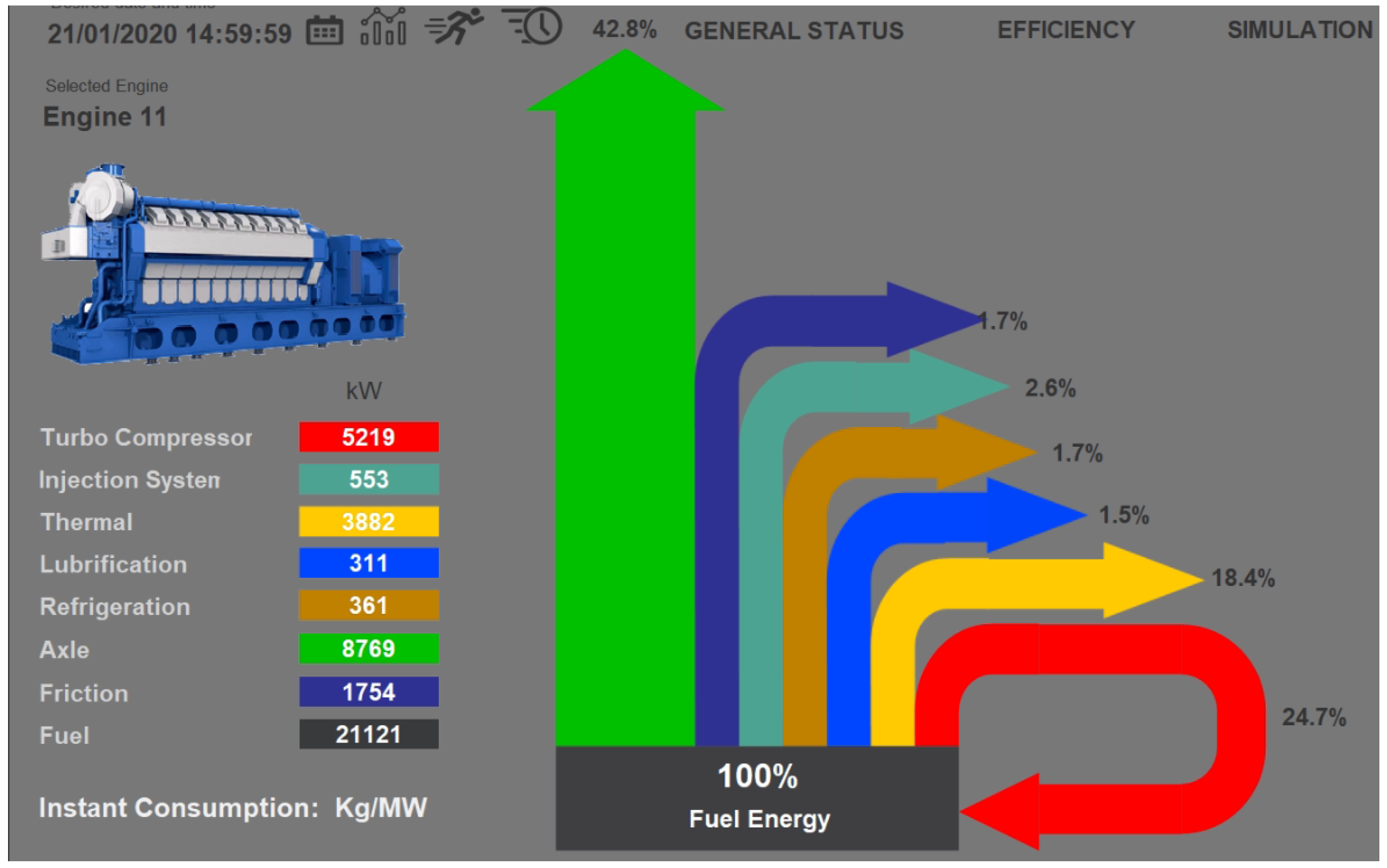
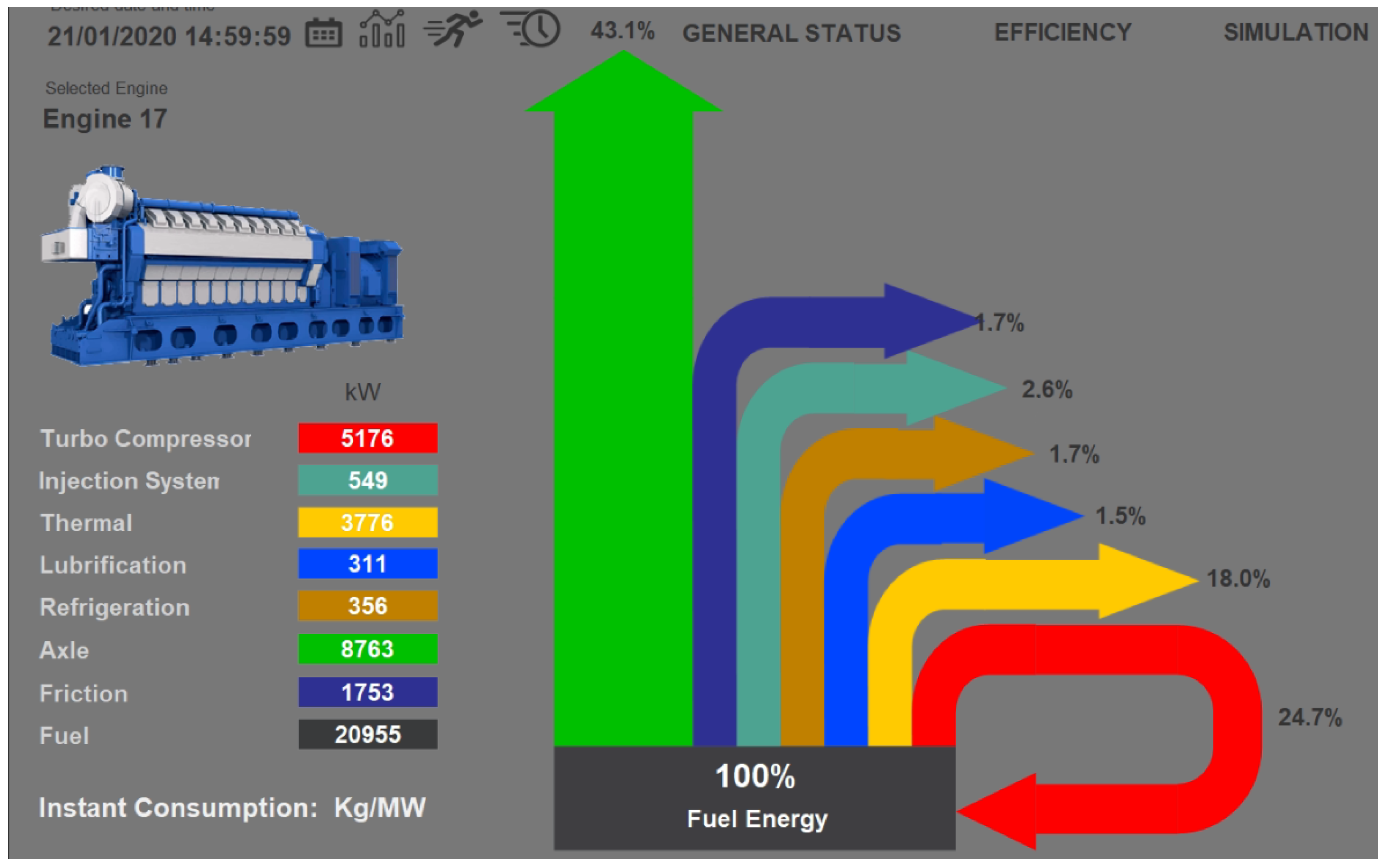
2.2. Sankey Diagram
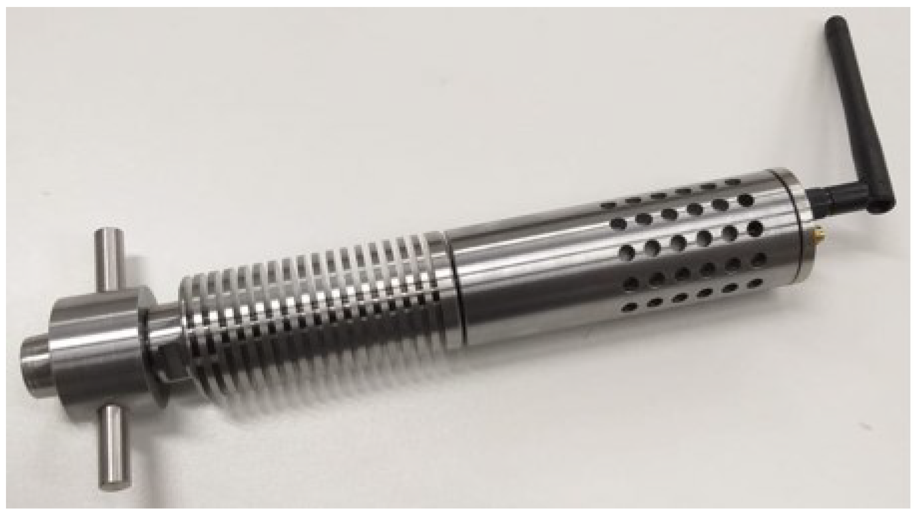
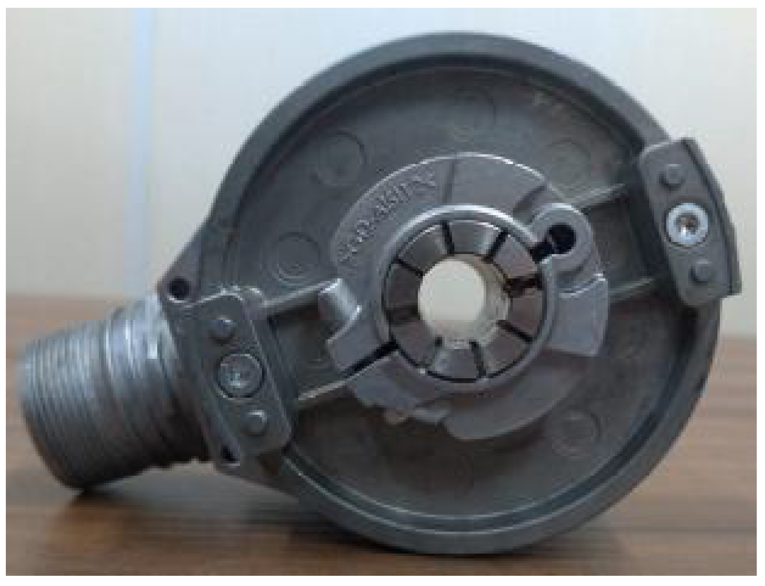
2.3. Complementary Instrumentation
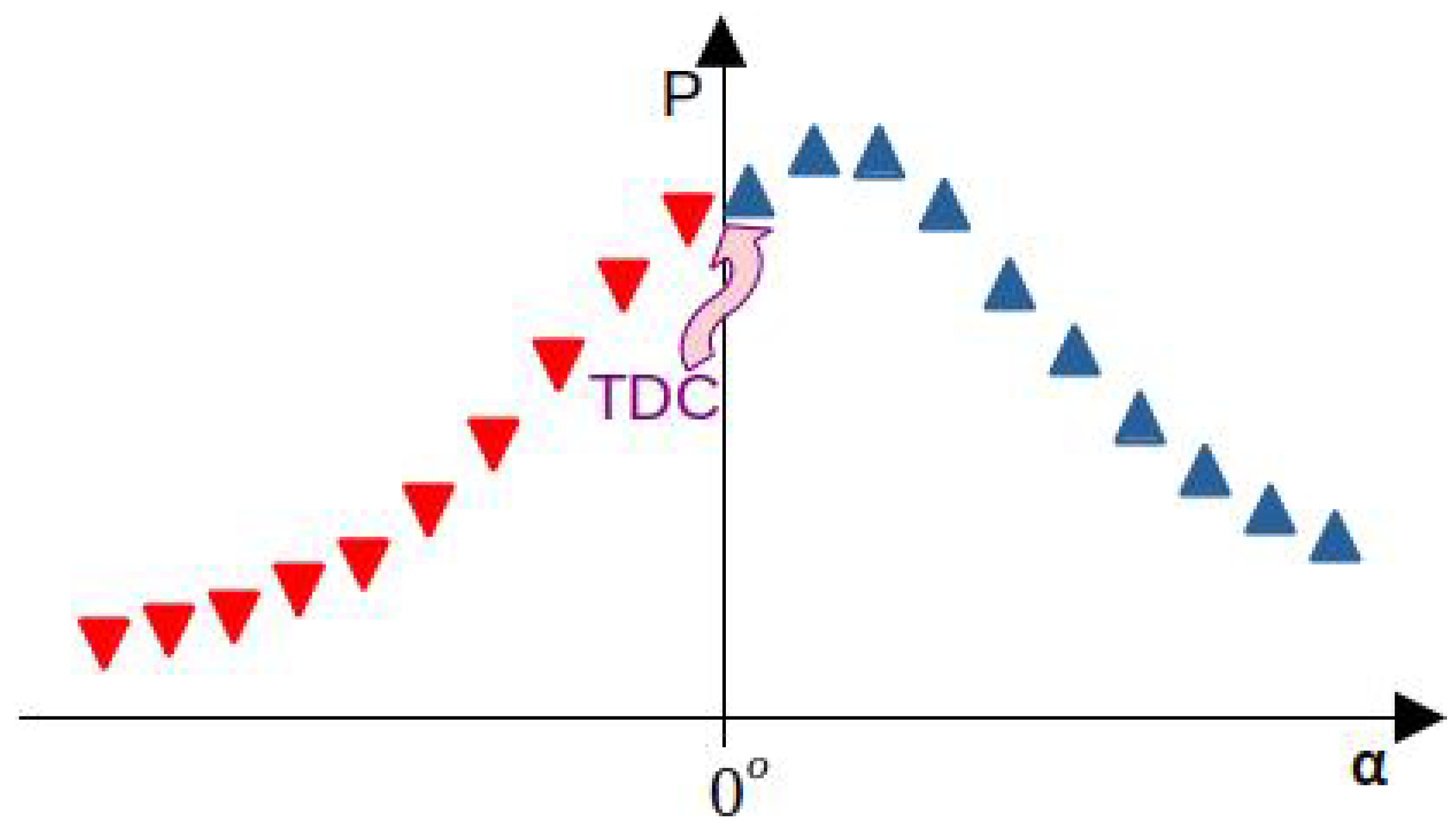
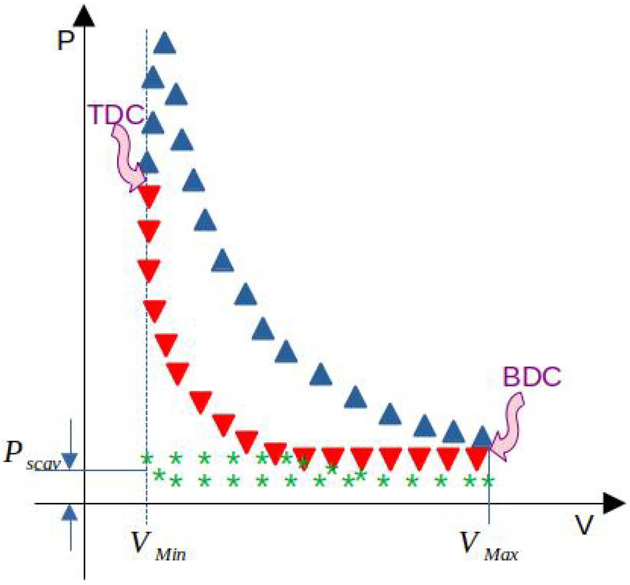
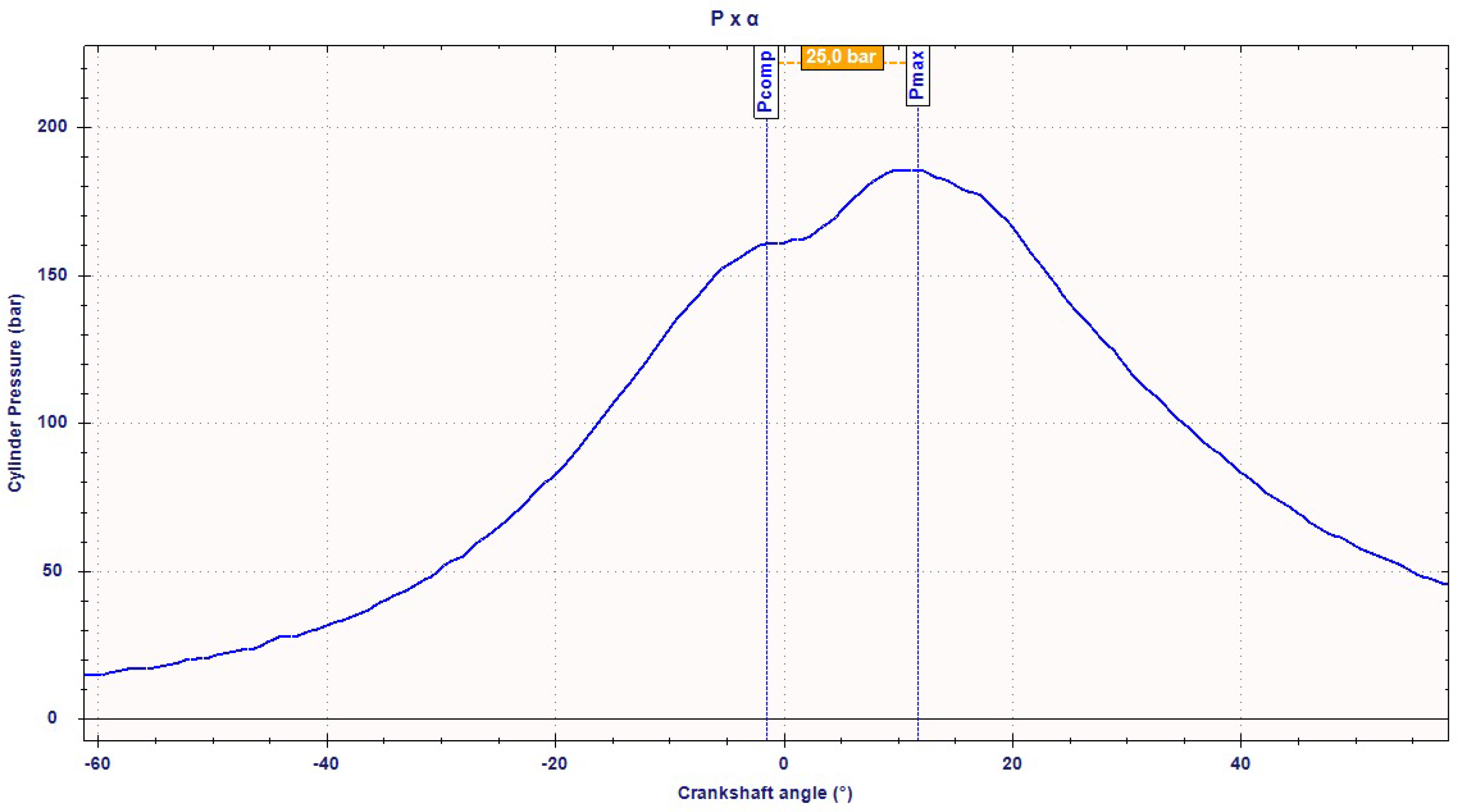
2.3.1. In-Cylinder Pressure Monitoring
2.3.2. Instant Speed Monitoring
2.4. Calculation Procedure
2.4.1. Consumed Injection Power
2.4.2. Consumed Cooling Power
2.4.3. Consumed Lubrication Power
2.4.4. Dissipated Heat
2.4.5. Turbocompressor Power
2.4.6. Other Consumed Power
3. Results and Discussion
3.1. Results at the Reduced Scale Laboratory
3.2. Results at the Pernambuco III Power Plant (Brazil)
4. Conclusions and Future Work
Author Contributions
Funding
Institutional Review Board Statement
Informed Consent Statement
Data Availability Statement
Acknowledgments
Conflicts of Interest
Abbreviations
| ANEEL | Brazilian Regulatory Agency for Energy |
| GD | Gas–Diesel |
| BDC | Bottom Dead Center |
| HFO | Heavy Fuel Oil |
| ICE | Internal Combustion Engine |
| LHV | Lower Heating Value |
| MIP | Mean Indicated Pressure |
| ONS | Brazilian Power System Operator |
| P | Pressure |
| PROCEL | Brazilian Program for Conservation of Electrical Energy |
| SIN | Brazilian National Interconnected System |
| TDC | Top Dead Center |
| TPP | Thermal Power Plant |
| V | Volume |
| WHR | Waste Heat Recovery |
| WOIS | Wärtsilä Operator’s Interface System |
References
- Santos, A.Q.; da Silva, A.R.; Ledesma, J.J.; de Almeida, A.B.; Cavallari, M.R.; Junior, O.H. Electricity Market in Brazil: A Critical Review on the Ongoing Reform. Energies 2021, 14, 2873. [Google Scholar] [CrossRef]
- ANEEL. Sistemas de Geracao da ANEEL-SIGA. Available online: https://www.gov.br/aneel/pt-br/centrais-de-conteudos/relatorios-e-indicadores/geracao#:~:text=SIGA%20%2D%20Sistema%20de%20Informa%C3%A7%C3%B5es%20de,reduzida%20com%20registro%20na%20Ag%C3%AAncia (accessed on 6 June 2022).
- Campos, M.M.; Borges-da-Silva, L.E.; Arantes, D.D.; Teixeira, C.E.; Bonaldi, E.L.; Lambert-Torres, G.; Ribeiro Junior, R.F.; Krupa, G.P.; Sant’Ana, W.C.; Oliveira, L.E.; et al. An Ultrasonic-Capacitive System for Online Characterization of Fuel Oils in Thermal Power Plants. Sensors 2021, 21, 7979. [Google Scholar] [CrossRef] [PubMed]
- Forman, C.; Muritala, I.K.; Pardemann, R.; Meyer, B. Estimating the global waste heat potential. Renew. Sustain. Energy Rev. 2016, 57, 1568–1579. [Google Scholar] [CrossRef]
- Mehmood, M.U.; Cho, S. Optimization of a Thermomagnetic Heat Engine for Harvesting Low Grade Thermal Energy. Energies 2021, 14, 5768. [Google Scholar] [CrossRef]
- Gonzalez-Ayala, J.; Guo, J.; Medina, A.; Roco, J.; Hernández, A.C. Energetic self-optimization induced by stability in low-dissipation heat engines. Phys. Rev. Lett. 2020, 124, 050603. [Google Scholar] [CrossRef]
- Gonzalez-Ayala, J.; Medina, A.; Roco, J.; Calvo Hernández, A. Thermodynamic optimization subsumed in stability phenomena. Sci. Rep. 2020, 10, 14305. [Google Scholar] [CrossRef]
- Gonzalez-Ayala, J.; Guo, J.; Medina, A.; Roco, J.; Hernández, A.C. Optimization induced by stability and the role of limited control near a steady state. Phys. Rev. E 2019, 100, 062128. [Google Scholar] [CrossRef]
- Ramousse, J.; Goupil, C. Chart for Thermoelectric Systems Operation Based on a Ternary Diagram for Bithermal Systems. Entropy 2018, 20, 666. [Google Scholar] [CrossRef]
- Agarwal, A.K.; Srivastava, D.K.; Dhar, A.; Maurya, R.K.; Shukla, P.C.; Singh, A.P. Effect of fuel injection timing and pressure on combustion, emissions and performance characteristics of a single cylinder diesel engine. Fuel 2013, 111, 374–383. [Google Scholar] [CrossRef]
- Costa, R.C.; Sodré, J.R. Compression ratio effects on an ethanol/gasoline fuelled engine performance. Appl. Therm. Eng. 2011, 31, 278–283. [Google Scholar] [CrossRef]
- Zhou, Y.; Tang, J.; Zhang, C.; Li, Q. Thermodynamic analysis of the air-cooled transcritical Rankine cycle using CO2/R161 mixture based on natural draft dry cooling towers. Energies 2019, 12, 3342. [Google Scholar] [CrossRef]
- Tang, J.; Zhang, Q.; Zhang, Z.; Li, Q.; Wu, C.; Wang, X. Development and performance assessment of a novel combined power system integrating a supercritical carbon dioxide Brayton cycle with an absorption heat transformer. Energy Convers. Manag. 2022, 251, 114992. [Google Scholar] [CrossRef]
- Payri, F.; Luján, J.M.; Martín, J.; Abbad, A. Digital signal processing of in-cylinder pressure for combustion diagnosis of internal combustion engines. Mech. Syst. Signal Process. 2010, 24, 1767–1784. [Google Scholar] [CrossRef]
- Luján, J.M.; Bermúdez, V.; Guardiola, C.; Abbad, A. A methodology for combustion detection in diesel engines through in-cylinder pressure derivative signal. Mech. Syst. Signal Process. 2010, 24, 2261–2275. [Google Scholar] [CrossRef]
- Morey, F.; Seers, P. Comparison of cycle-by-cycle variation of measured exhaust-gas temperature and in-cylinder pressure measurements. Appl. Therm. Eng. 2010, 30, 487–491. [Google Scholar] [CrossRef]
- Ahmadi, M.H.; Alhuyi Nazari, M.; Sadeghzadeh, M.; Pourfayaz, F.; Ghazvini, M.; Ming, T.; Meyer, J.P.; Sharifpur, M. Thermodynamic and economic analysis of performance evaluation of all the thermal power plants: A review. Energy Sci. Eng. 2019, 7, 30–65. [Google Scholar] [CrossRef]
- Kaushik, S.C.; Reddy, V.S.; Tyagi, S.K. Energy and exergy analyses of thermal power plants: A review. Renew. Sustain. Energy Rev. 2011, 15, 1857–1872. [Google Scholar] [CrossRef]
- Leach, F.; Kalghatgi, G.; Stone, R.; Miles, P. The scope for improving the efficiency and environmental impact of internal combustion engines. Transp. Eng. 2020, 1, 100005. [Google Scholar] [CrossRef]
- Konieczna, A.; Roman, K.; Borek, K.; Grzegorzewska, E. GHG and NH3 Emissions vs. Energy Efficiency of Maize Production Technology: Evidence from Polish Farms; a Further Study. Energies 2021, 14, 5574. [Google Scholar] [CrossRef]
- Assuncao, F.D.O.; Borges-da-Silva, L.E.; Villa-Nova, H.F.; Bonaldi, E.L.; Oliveira, L.E.L.; Lambert-Torres, G.; Teixeira, C.E.; Sant’Ana, W.C.; Lacerda, J.; da Silva Junior, J.L.M.; et al. Reduced Scale Laboratory for Training and Research in Condition-Based Maintenance Strategies for Combustion Engine Power Plants and a Novel Method for Monitoring of Inlet and Exhaust Valves. Energies 2021, 14, 6298. [Google Scholar] [CrossRef]
- Texas Instruments. CC3200 Simple-Link Wi-Fi and Internet-of-Things Solution, a Single Chip Wireless MCU Technical Reference Manual. Available online: https://www.ti.com/lit/ug/swru367d/swru367d.pdf (accessed on 6 June 2022).
- Niemi, S. Survey of Modern Power Plants Driven by Diesel and Gas Engines. 1997. Available online: https://www.osti.gov/etdeweb/biblio/628799 (accessed on 6 June 2022).
- Ogasawara, H.; Takai, M. Fuel Injection Timing Control System for a Diesel Engine. U.S. Patent US 4,388,909, 21 July 1983. [Google Scholar]
- Jankowski, A.; Kowalski, M. Environmental Pollution Caused by a Direct Injection Engine. J. Kones 2015, 22. [Google Scholar] [CrossRef]


| Diameter of cylinder (mm) | 320 |
| Course of cylinder (mm) | 400 |
| Volume of cylinder (m) | 0.03217 |
| Number of intake valves | 2 |
| Number of outtake valves | 2 |
| Number of cylinders | 20 |
| Engine speed/rotation (rpm) | 750 |
| Average speed of cylinders (m/s) | 10 |
| Average power per cylinder (kW) | 580 |
| Viscosity of fuel at 50 C (cSt) | 2-730 |
| Test Condition of Fuel Injection Pump | Fuel Consumption | Generated Energy |
|---|---|---|
| out of adjustment | 3920 mL | 7.170 kWh |
| regulated position | 3650 mL | 7.304 kWh |
| Cylinder (Test Condition) | MIP |
|---|---|
| Cylinder 1 (unregulated pump) | 8.4 bar |
| Cylinder 2 (unregulated pump) | 7.6 bar |
| Cylinder 3 (unregulated pump) | 9.3 bar |
| Cylinder 4 (unregulated pump) | 7.9 bar |
| Cylinder 1 (regulated pump) | 8.6 bar |
| Cylinder 2 (regulated pump) | 8.1 bar |
| Cylinder 3 (regulated pump) | 9.4 bar |
| Cylinder 4 (regulated pump) | 7.8 bar |
Publisher’s Note: MDPI stays neutral with regard to jurisdictional claims in published maps and institutional affiliations. |
© 2022 by the authors. Licensee MDPI, Basel, Switzerland. This article is an open access article distributed under the terms and conditions of the Creative Commons Attribution (CC BY) license (https://creativecommons.org/licenses/by/4.0/).
Share and Cite
Ramos, L.C.; Assuncao, F.d.O.; Villa-Nova, H.F.; Lambert-Torres, G.; Bonaldi, E.L.; Oliveira, L.E.d.L.d.; Sant’Ana, W.C.; Junior, R.F.R.; Teixeira, C.E.; Medeiros, P.G.P.d. Proposal of a System to Identify Failures and Evaluate the Efficiency of Internal Combustion Engines of Thermal Power Plants. Energies 2022, 15, 9047. https://doi.org/10.3390/en15239047
Ramos LC, Assuncao FdO, Villa-Nova HF, Lambert-Torres G, Bonaldi EL, Oliveira LEdLd, Sant’Ana WC, Junior RFR, Teixeira CE, Medeiros PGPd. Proposal of a System to Identify Failures and Evaluate the Efficiency of Internal Combustion Engines of Thermal Power Plants. Energies. 2022; 15(23):9047. https://doi.org/10.3390/en15239047
Chicago/Turabian StyleRamos, Lilia Carneiro, Frederico de Oliveira Assuncao, Helcio Francisco Villa-Nova, Germano Lambert-Torres, Erik Leandro Bonaldi, Levy Ely de Lacerda de Oliveira, Wilson Cesar Sant’Ana, Ronny Francis Ribeiro Junior, Carlos Eduardo Teixeira, and Paulo Germano Pinto de Medeiros. 2022. "Proposal of a System to Identify Failures and Evaluate the Efficiency of Internal Combustion Engines of Thermal Power Plants" Energies 15, no. 23: 9047. https://doi.org/10.3390/en15239047
APA StyleRamos, L. C., Assuncao, F. d. O., Villa-Nova, H. F., Lambert-Torres, G., Bonaldi, E. L., Oliveira, L. E. d. L. d., Sant’Ana, W. C., Junior, R. F. R., Teixeira, C. E., & Medeiros, P. G. P. d. (2022). Proposal of a System to Identify Failures and Evaluate the Efficiency of Internal Combustion Engines of Thermal Power Plants. Energies, 15(23), 9047. https://doi.org/10.3390/en15239047