Impact of Time Resolution on Curtailment Losses in Hybrid Wind-Solar PV Plants

Abstract

Curtailment losses for large-scale hybrid wind–solar photovoltaic (PV) plants with a single grid connection point are often calculated in 1 h time resolution, underestimating the actual curtailment losses due to the flattening of power peaks occurring in shorter time frames. This paper analyses the curtailment losses in hybrid wind–PV plants by utilising different time resolutions of wind and PV production while varying the grid cut-off power, wind/solar PV farm sizes, and shares of wind/PV capacity. Highly resolved 1 s measurements from the operational wind farm and pyranometer are used as an input to specialized wind and PV farm power production models that consider the smoothing effect. The results show that 15 min resolution is preferred over 1 h resolution for large-scale hybrid wind–PV plants if more accurate assessment of curtailment losses is required. Although 1 min resolution additionally increases the estimation accuracy over 15 min resolution, the improvement is not significant for wind and PV plants with capacity above approx. 10 MW/10 MWp. The resolutions shorter than 1 min do not additionally increase the estimation accuracy for large-scale wind and PV plants. More attention is required when estimating curtailment losses in wind/PV plants with capacity below approx. 10 MW/10 MWp, where higher underestimation can be expected if lower time resolutions are used.

1. Introduction

The wind and solar photovoltaic (PV) installed capacity growth is showing staggering rates over the past decades while currently being at competitive or lower prices than conventional power plants [1]. Considering the intermittent nature of variable renewable sources (VREs), integration of wind and solar PV plants into hybrid power plants (HPPs) is a viable option for increased decarbonization and net-zero emissions by 2050 [2]. The local complementary nature between wind and solar resources enables hybrid wind–solar plants to produce energy more efficiently in comparison with individual wind or PV plants [3]. However, during the HPP development process, special attention must be dedicated to data used for techno-economic analysis and other aspects [4]. One of the important data-driven decisions is to assess whether the wind and solar resources on-site are negatively correlated, thus allowing for efficient utilization of both VRE sources.

Hybrid wind–solar plants have multiple advantages over pure wind or solar PV plants, including but not limited to, more efficient grid utilization and land use, decreased grid infrastructure, project development, and balancing costs [5]. As emphasized in [5], the only way to fully exploit the HPPs is to install higher wind–solar capacity than the agreed grid connection capacity. Thus, system planners need to design HPP in such a way that the curtailment losses, which occur whenever the potential wind and solar generation exceeds the grid connection capacity (grid cut-off power), are sustained at acceptable levels. The grid curtailment is assumed to occur instantly, i.e., the HPP control system reduces the power output of either the solar or wind farm whenever HPP instantaneous power production is above the grid cut-off power. However, when curtailment estimation studies are prepared, planners are often limited with low-resolution data, which forces them to deliver calculations in 10 min, 15 min, or most frequently, 1 h averaged time resolutions. The averaging process causes loss of information about the power fluctuations inside the interval and flattens the power peaks occurring in shorter time frames [6]. Power peaks of wind and solar generation inside the averaging interval can cause the potential HPP power to exceed grid cut-off power and introduce curtailment losses, while simultaneously the average power will not. Therefore, the use of lower time resolutions will underestimate actual curtailment losses.

The literature related to HPPs is very broad. Between 1995 and 2020, 550 papers about hybrid power plants were published, of which 168 papers focus on grid-connected systems [7]. A review paper by Lindberg et al. [8] has summarized the key findings related to utility-scale wind–solar PV HPPs, and pointed out that the research field of HPPs is relatively immature. The majority of papers addressed complementarity characteristics between wind and solar PV plants [9] or solar and wind resources in different areas [10,11,12]. The researchers have shown that the complementarity of wind and solar resources globally have considerable potential for the implementation of wind–solar HPPs in future power systems. Several papers have also addressed the hybridization of existing wind farms with solar PV capacity. In Ref. [13], authors have proposed a multi-objective optimization model for the expansion of existing wind farms with solar PV capacity to reduce power output fluctuations, optimize electrical equipment, and limit curtailment losses. Silva and Estanqueiro [14] have focused on the energetic contribution and economic feasibility of converting existing wind farms into HPPs and showed that expansion with solar capacity can be economically more efficient in contrast to pure wind capacity. In Ref. [15], the authors have conducted a techno-economic feasibility study of adding offshore floating solar PV capacity to the offshore wind farm in the North Sea while having limited cable capacity.

Only a few papers have dealt with curtailment losses in large-scale hybrid wind–solar PV plants in more detail. Ludwig et al. [6] quantified the curtailment losses for different shares of wind and PV capacity in HPP and various grid connection capacities. Curtailment losses were calculated in hourly averaged time resolution, while supplementary evaluations of curtailment losses in 1 min resolution were provided for a pure PV plant to inspect additional curtailment losses. Grab et al. [16] have analysed the curtailment losses in HPP consisting of a 24 MW wind farm and a 10.3 MWp solar PV farm located in Eastern Germany. The authors have used 5 s power measurements at the 20 kV feeders, but downsampled the data to 1 min resolution before calculating curtailment losses. However, a comparative analysis of curtailment losses in different time resolutions has not been provided. In Ref. [17], curtailment analysis for 10 existing wind farms across Australia has been examined. The analysis has showed that wind farms can be expanded with solar PV plants having a capacity between 25% and 50% of wind farm capacity while limiting PV curtailment losses to 5%. Calculations of the solar PV part were based on the hourly irradiance data and PVSyst modelling software. Couto and Estanqueiro [18] have considered the expansion of existing wind farms in Portugal with additional pure wind, pure solar PV, and combined wind and solar PV capacity without grid reinforcement. The paper has found that expanding existing wind farms with additional 50% solar PV capacity results in maximum 5% curtailment (% of total HPP production), compared to equivalent 30% curtailment when the same wind capacity is added. The calculations are provided also in hourly resolution. Contrary to the most of existing analysis, in the WindEurope position paper it is recommended that “curtailment estimation studies need to be deployed on 10-min or 15-min basis to be reliable for decision making” [5], referring to [19]. The rationale behind the requested time resolution is not provided. In addition, previous general recommendations on time resolution do not account for the wind and solar PV farm installed capacity. Larger wind and solar PV farms will reduce the power fluctuations due to the so-called smoothing effect [20], thus affecting additional curtailment losses.

To the best of the authors’ knowledge, none of the existing research has compared the curtailment losses in different time resolutions for hybrid wind–solar PV farms. It is unknown to what extent the actual curtailment losses will differ from the curtailment losses estimated in lower time resolutions (e.g., 1 h or 15 min). Moreover, the impact of the wind and solar PV farm size on the reduction of power fluctuations and indirectly on curtailment losses has not been studied either. Existing papers often overlook the importance of wind and solar PV farm size and the smoothing effect by scaling the power of wind/PV farms with a constant to analyse the curtailment losses with different shares of wind and solar PV capacity. While this procedure can be applied when using low resolution time series, its use on highly resolved time series (e.g., time resolutions below 10-min) will introduce artificial fluctuations in higher frequency spectrum and overestimate actual power fluctuations, especially on larger power plants.

The main goal of this paper is to provide detailed calculations of curtailment losses in large-scale hybrid wind–solar PV farms when different time resolutions for output power time series are utilised. The curtailment losses are examined by considering grid connection capacity, wind/PV farm sizes, and different shares of wind/PV capacity in HPP. The calculations are made by utilising highly-resolved 1 s data measured at a wind farm and pyranometer as an input to specialized wind and solar PV power production models. The power output of the models is resampled to various time resolutions, allowing the comparison of curtailment losses in different resolutions.

This research paper brings novelty by introducing the methodology for calculation of curtailment losses in large-scale hybrid wind–solar PV plants with the use of scalable wind and solar PV models that consider the smoothing effect, thus allowing the examination of curtailment losses with various wind and PV plant sizes. Furthermore, the quantitative comparison of curtailment losses in different time resolutions used for wind and PV power production is provided. The insight gained from the analysis and the guidelines on the adequate time resolution will provide the researchers or HPP planners with valuable information when evaluating the curtailment losses in hybrid wind–PV plants.

The basic outline of the work is represented as the flowchart depicted on Figure 1. The respective parts of the figure are further elaborated in the sections as follows. Section 2 and Section 3 introduce the scalable wind and solar PV power production models and data processing involved for each technology. Section 4 describes the methodology behind curtailment losses calculation. Section 5, Section 6 and Section 7 present the results, the discussion, and conclusions, respectively.

2. Wind Farm Power Production Analysis

2.1. Wind Farm Dataset

The data were collected from an operational wind farm in Croatia which has 49 MW installed capacity, consisting of wind turbine generators (WTGs) with 3200 kW and 2850 kW rated power. The wind turbines are three-bladed, horizontal-axis type with rotor diameter of 103 m and a hub height of 98.3 m. A multi-stage planetary gearbox is used to convert low-rpm main shaft torsional power to a double fed induction generator (DFIG) with a partial power converter system in the rotor circuit. The power converter system consists of an AC/DC converter on the rotor side, DC intermediate circuit, and power inverter on the 0.69 kV low voltage (LV) grid side. The nominal voltage in stator circuit is 6 kV. The power is exported to the grid via 33/6/0.69 kV three-winding step-up transformer and a medium voltage (MV) switchgear located in the bottom of the tubular steel tower.

The data are collected by Supervisory Control and Data Acquisition System which contains 1 s WTG active power and wind speed measurements from the wind sensor located at the top of the nacelle, for each WTG, spanning over the whole year of 2021, excluding December. The active power measured from the WTGs corresponds to the net active power produced that includes the consumption of internal WTG systems, without considering the losses in 33/6/0.69 kV WTG transformer. To compensate for the WTG transformer and 33 kV internal cable grid losses, wind farm power output in the later stage is corrected with 1.5% fixed losses.

On average, the dataset availability for the WTG power is 89.5% for January and February (the first four days in January are missing), 96.4% for March–May, 96.7% for June–August, and 96.4% for September–November. The technique used to handle missing values is important for the analysis of curtailment losses. In the analysed data, missing values appear most commonly one interval at a time (1 s missing intervals), often with subsequent missing values every few intervals (rarely continuously during longer intervals). The pattern in which missing values appear is completely random and generally does not occur simultaneously on multiple WTGs. The exception is when values are missing over longer periods (four days in January), in which case they do occur on all WTGs.

The missing values can either be deleted or imputed. Deleting missing data points, in this case, is problematic as they do not appear simultaneously across multiple WTGs. Hence, linear interpolation is used to handle missing data separately for each WTG. It has to be emphasized that linear interpolation will neglect the fluctuation levels inside the interpolated interval, thus possibly reducing power peaks. As missing values appear most frequently one value at time, it should not have a significant influence on possible reductions of additional curtailment losses. Furthermore, the influence is only important during periods when both wind and solar PV production is high enough so that curtailment can occur.

2.2. Power Fluctuations in Wind Farms

The WTG inertia, along with different production profiles between WTGs in the wind farm, perform an active role in the reduction of wind farm power fluctuations. The analysis of power fluctuations and smoothing effect in wind farms is an important aspect for curtailment estimation. In this paper, the power fluctuations are analysed by utilising the ratio of the standard deviation (normalized or non-normalized) of aggregated WTGs power to that of a single WTG power. In the literature, this ratio is called smoothing effect index (SEI) [21]. In this context, a non-normalized variant of SEI is used to describe the power fluctuations in wind farms.

Since the aim of this paper is to explore the curtailment losses in wider frequency range, the standard deviation of power fluctuations is calculated on various frequency scales by using the Maximal Overlap Discrete Wavelet Transform (MODWT). The goal is to decompose the wind power time series of aggregated WTGs to multiple frequency scales, where each scale represents power fluctuations at a specific frequency range, and calculate the SEI on a scale-basis (i.e., SEI for each frequency scale). Hence, in the subsequent section, a brief introduction to MODWT is provided.

2.2.1. Maximal Overlap Discrete Wavelet Transform

MODWT is a type of wavelet transform that provides a time-scale representation of the time series and allows for variance decomposition. It essentially translates the time series through various high- and low-pass filters, separating the high-frequency components at each level and the lowest frequency component at the final level. In contrast to discrete wavelet transform (DWT), it does not suffer from certain drawbacks, as noted in [22]. Namely, the MODWT does not require the time series to have a length equal to $2^n$, where n is an integer. Moreover, when decomposing the time series, each produced scale has a length equal to the analysed time series (in contrast to DWT, downsampling is avoided). Hence, when applied to a time series with length T, MODWT produces $J_0$ new time series, each with the same length T. The $J_0$ represents the number of levels or scales of the MODWT. Given the time series $y_t, t=1,\dots ,T$, the variance decomposition of the y is given by the following equation [22]:

$${\left|\right|y\left|\right|}^2=\sum _{j=1}^{J_0}\left|\right|W_j{\left|\right|}^2+\left|\right|V_{J_0}{\left|\right|}^2,$$

(1)

where $\left|\right|·\left|\right|$ is the vector norm, $W_j$ are the wavelet coefficients, $V_{J_0}$ are the final level scaling coefficients. Thus, MODWT decomposes the variance to scales $j=1,\dots ,J_0$ such that the sum of the variances of each scale is equal to the variance of the time series y.

Details of wavelet variance estimation, boundary conditions, and confidence intervals are given in [23]. Additionally, both DWT and MODWT can be used for performing the multiresolutional analysis (MRA), a scale-based additive decomposition of the time series y [22]:

$$y=\sum _{j=1}^{J_0}{D}_j+S_{J_0},$$

(2)

where $D_j$ and $S_{J_0}$ are detail and final-level smoothing coefficients, respectively. Here, time series y is transformed into multiple time-adjusted time-series. While MODWT is variance preserving, MRA based of MODWT is additive decomposition, and as such, detail and smoothing coefficients cannot be used for the analysis of variance [22]. In this paper, python implementation of the MODWT based on [24] is used.

2.2.2. Power Fluctuations and Smoothing Effect

The MODWT is used to derive scale-based SEI in an approach previously used by the authors in [25] to inspect power fluctuations and smoothing effects in wind farms. The SEI as the representation of power fluctuations on various frequency scales is analysed by (a) aggregating power time series of N = 1, 2, …, M wind turbines, where M is the total number of WTGs in wind farm; (b) for each N, MODWT is applied on aggregated power time series to obtain multiple time scales representations; (c) estimating wavelet variance (unbiased estimation according to [23]) for each scale; (d) SEI calculation by taking the square root of previously-obtained variances.

In Figure 2, the SEI as a function of aggregated WTGs in wind farm is represented for scales 1 and 2 (high frequency), 9 and 10 (medium frequency), and 15 and 16 (low frequency). When 1 s data are used, the first scale represents the power fluctuations with the periods between 2–4 s, the second scale 4–8 s, etc. The SEI function is fitted with a function $N^{\alpha }$, obtaining $\alpha$ for each scale. It can be observed that the SEI tends to increase by a factor of $\sqrt{N}$ ($\alpha =0.5$) for higher frequency power fluctuations and N (linear increase, $\alpha =1.0$) for lower frequency fluctuations. In general, the increase of SEI for a specific frequency scale can be described by the function $N^{\alpha }$, where $\alpha$ is termed as “smoothing exponent”.

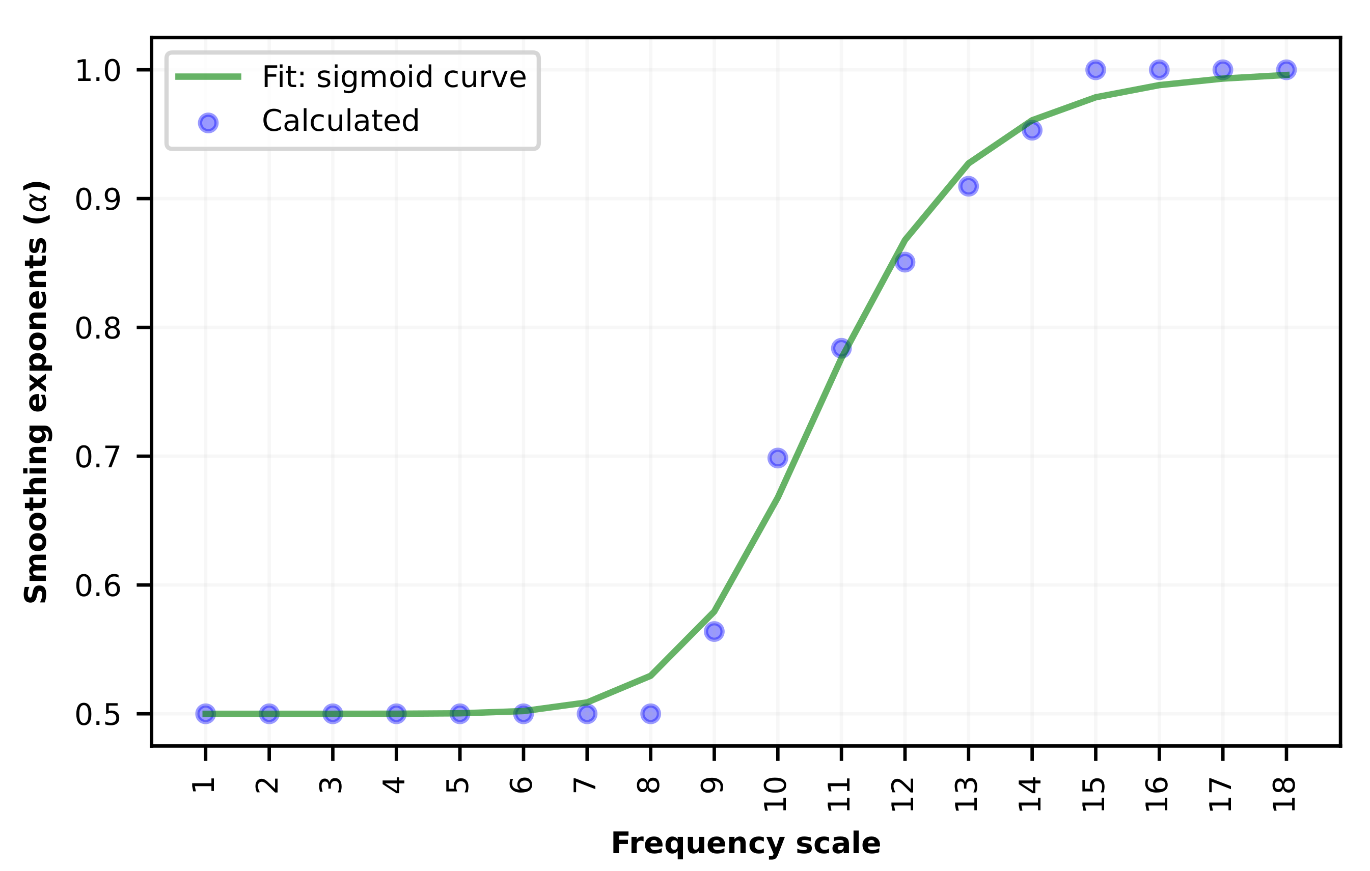
Calculated smoothing exponents are shown for each frequency scale and for the month of April in Figure 3. High levels of smoothing are observable for the first eight scales (periods of fluctuations up to $2^8=256$ s), after which smoothing exponents rise (smoothing effect slowly starts to reduce), finally reaching a value of $\alpha =1.0$ at scale 15 (periods of fluctuations between $2^{15}$–$2^{16}$ s, approx. 9–18 h). Calculated smoothing exponents at scales <=5 and >=15 are rounded to 0.5 and 1.0, respectively, as smoothing exponents at respective scales fluctuate around those values within $\pm 5$%.

Smoothing exponents for various scales can be fitted with a sigmoid function (a and b being the parameter of the sigmoid function) of the form:

$$S(a,b)=1-{\displaystyle \frac{0.5}{1+{\left(\frac{x}{a}\right)}^b}}.$$

(3)

The smoothing exponents can be used to study the smoothing effect in wind farms, which is important for the analysis of curtailment losses. Smoothing exponents are constrained between 0.5 and 1.0, where 0.5 represents the maximum theoretical smoothing effect (negligible correlations between WTGs power) and 1.0 represents non-smoothing conditions (WTGs power production profile is identical) on corresponding frequency scales.

Previous papers [26,27] show that the maximum theoretical smoothing effect in wind farms can be observed for periods of fluctuations below approximately 100 s, independently on the number of WTGs in the wind farm. Generally, the frequency scales at which smoothing effects in wind farms approach maximum/minimum theoretical limits can also slightly change depending on the wind farm terrain complexity and the distance between WTGs, as noted by the authors in [25]. Small changes between smoothing exponent curves can also be expected for different seasons.

The wind farm analysed in this paper shows high levels of smoothing due to the relatively high distance between WTGs and terrain complexity. The smoothing exponents derived from wind farm, on a month-by-month or quarterly basis, will be used in the following section to form the wind farm production model.

2.3. Wind Farm Model

To investigate the impact of wind farm installed capacity on the curtailment losses, a wind farm power scaling model is needed to overcome the obstacle of a limited number of WTGs. While the model can scale the power of WTG to an arbitrary multiple of its nominal power, it must replicate the wind farm power fluctuations (smoothing effect). The use of the model also enables to hedge the problems with WTG unavailability during larger periods (e.g., faults in WTG) or maintenance and underperformance issues that would not be taken into account in the curtailment estimation phase.

The wind farm production model, based on the production of the single WTG, is presented in more detail in the following sections.

2.3.1. Power Scaling Methodology

The starting point of the model is to choose the representative WTG for the specific period, since the wind farm model will depend on the WTG power production time series. Therefore, it is important to choose the WTG that was neither in the maintenance period nor had significant underperformance in the given interval.

It has to be emphasized that wind farm power production cannot be simply obtained by multiplying the power production of a single WTG with the number of WTGs, N, because the smoothing effect explained in Section 2.2 will reduce power fluctuations differently on various frequency scales. In other words, the power fluctuations of wind farm with N WTGs are reduced compared to single WTG power upscaled with N. The simple power scaling is possible only on lower frequency scales, where an increase in power fluctuations with each additional WTG is linear (as shown previously, this can be done for power fluctuations with the period above 9 h for the analysed wind farm). Other higher and medium frequency scales cannot be scaled linearly, otherwise, artificial fluctuations will be introduced in the power production profile of modelled wind farm power.

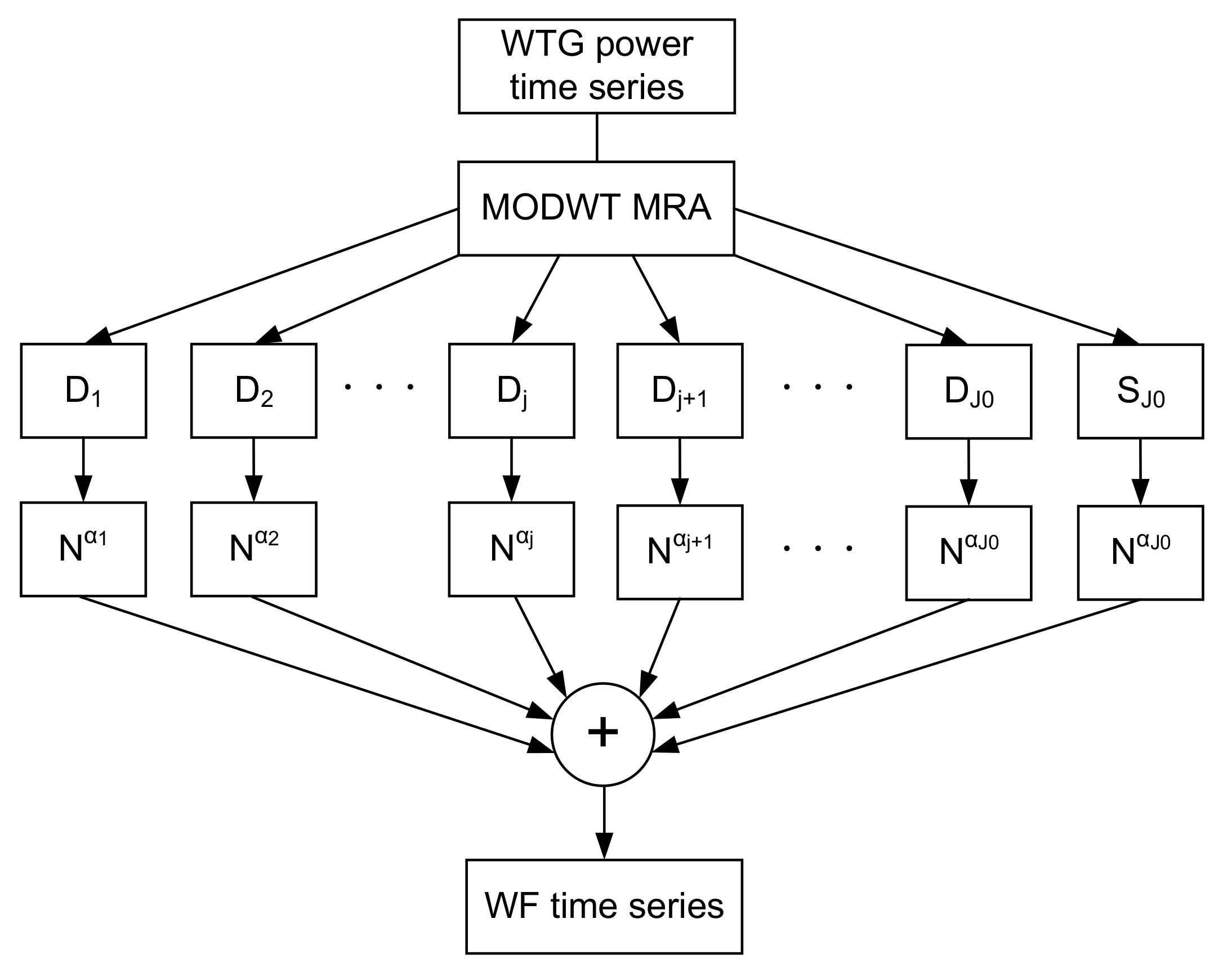
The basic idea behind the proposed wind farm power production model is to take into account the smoothing effect applied over various scales by multiplying each time-adjusted frequency scale with the corresponding SEI and aggregating the power time series of each scale. The time-adjusted frequency scales are obtained by applying MODWT based MRA, which is an additive transform.

To achieve this, the following algorithm is used:

• MODWT MRA is applied on WTG power time series, creating $J_0$ additive scales;
• Each scale is multiplied by the SEI values calculated from Section 2.2.2;
• Finally, scales are aggregated and wind farm power production profile is generated.

More formally, wind farm power generation of N aggregated WTGs is obtained as:

$$P_{t,N}^{WF}=\sum _{j=1}^{J_0}{D}_{jt}\times N^{{\alpha }_j}+S_{J_0}\times N^{{\alpha }_{J_0}},\forall t\in T.$$

(4)

Here, $D_{jt}$ and $S_{J_0}$ are detail coefficients and final-level smoothing coefficients of WTG power, respectively, and T is the length of the time series. The process of obtaining wind farm model is graphically represented in Figure 4.

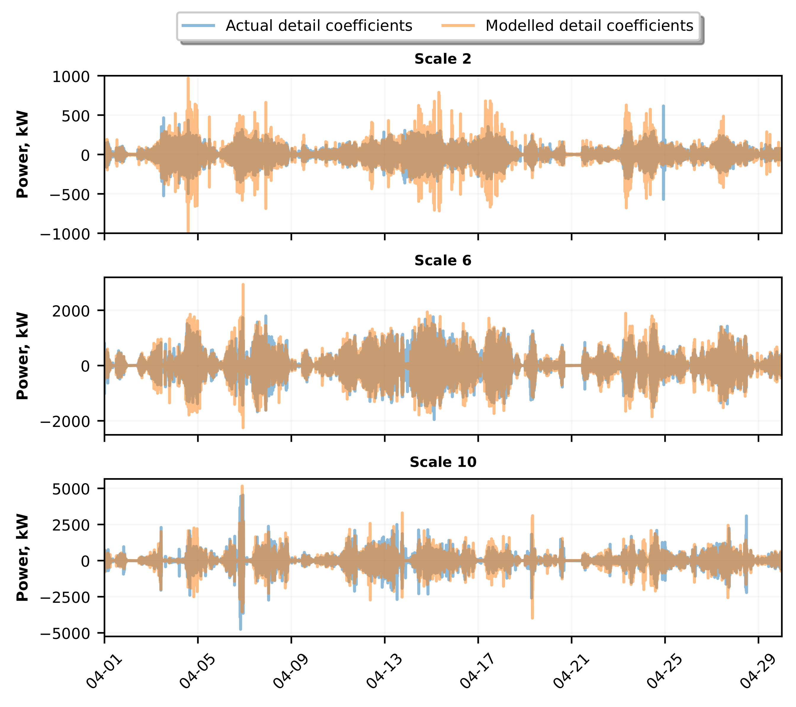
Figure 5 compares detail coefficients on scales 2, 6, and 10 of eight (8) aggregated WTGs and those obtained by the model using scale-based SEI values as a multiple of single WTG detail coefficients.

It can be seen that the model accurately captures the power fluctuations on lower-frequency scales (especially scale 10), but fails to capture fluctuations on the high-frequency scales (scale 2), While variance on high-frequency scale is similar between the actual and the modelled power production, the amplitude of the power fluctuations is not captured. Thus, a different approach to the problem is required on higher frequency scales to increase the accuracy of the method.

2.3.2. Surrogate Method for High Frequency Scales

To solve the problem on high-frequency scales, a different approach based on the surrogate time series method is used. The method tries to preserve important statistical properties of the detail coefficients. As it can be seen from the Figure 5, the high-frequency fluctuations of aggregated WTGs are locally decorrelated (i.e., amplitudes of high-frequency power fluctuations rarely appear simultaneously on multiple WTGs), but in general show similar long term trends (periods of higher and lower local variance). Therefore, the idea is to create multiple realisations (i.e., N multiples) of the detail coefficients with locally decorrelated structures, but similar variance trends. In this way, imitation of high-frequency detail coefficients can be obtained.

The time-series surrogate method based on this principle has been proposed by Nakamura and Small [28] and named small shuffle surrogate (SSS) method. In contrast to random shuffle of time series, this method shuffles the indices of the time series locally by the addition of Gaussian random numbers multiplied with an amplitude parameter, defining the locality of the shuffled data (the higher the amplitude parameter, the larger proportion of data is shuffled).

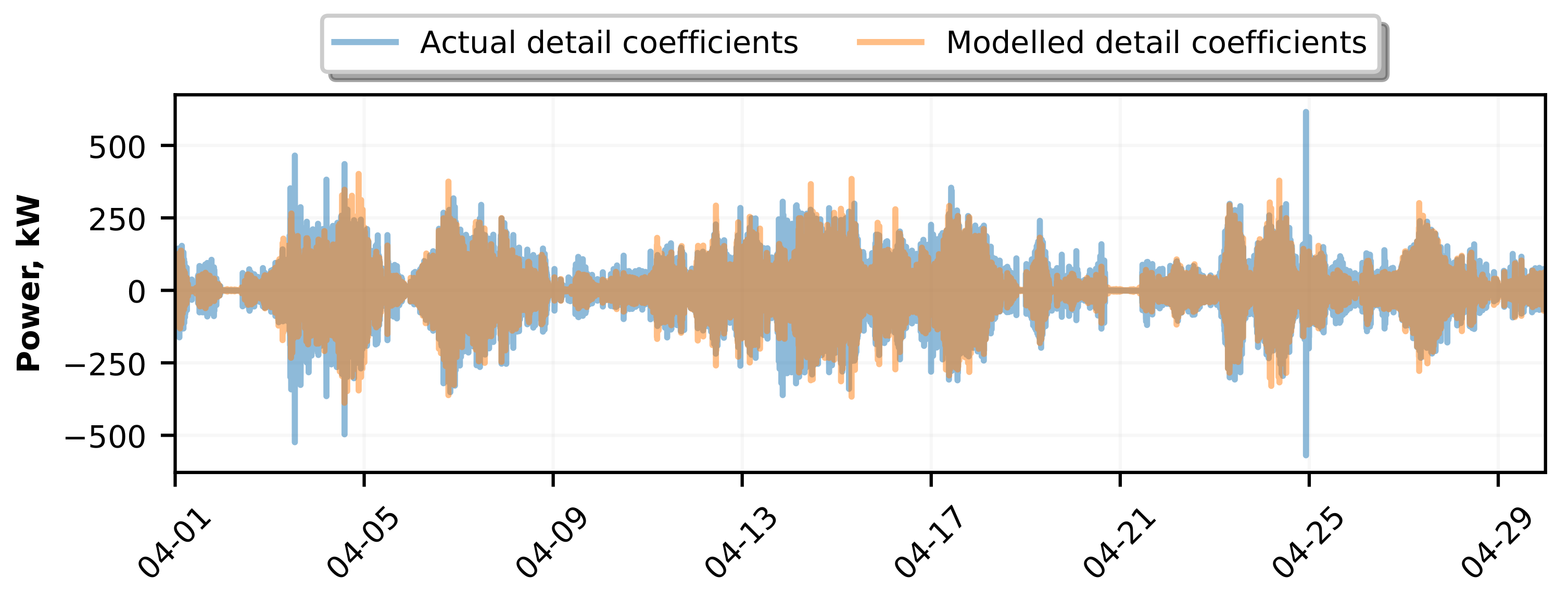
Although the mathematical background of this method is taken, the method is slightly modified in this implementation. More precisely, steps (i) and (iii) from SSS method are reproduced, but instead of rank-ordering in step (ii), the surrogate indices obtained from step (i) are sorted, and surrogate time series are obtained by reordering with sorted surrogate indices in step (iii). The surrogate indices that have values lower than zero and higher than the maximal index of the time series are replaced with original indices. Therefore, the local values at the start and the end of the time series remain unchanged. This process is repeated N times on the same detail coefficients of the WTG to obtain detail coefficients of the N aggregated WTGs. The results of this method are illustrated on the scale 2 in Figure 6. Note that the amplitude of the power fluctuations is now well captured.

The wind farm model introduced in the previous section can be expanded by applying the surrogate model on the k highest frequency scales (i.e., first k frequency scales), in the following manner:

$$P_{t,N}^{WF}=\sum _{j=1}^k\widehat{D_{jt}}+\sum _{j=k+1}^{J_0}{D}_{jt}\times N^{{\alpha }_j}+S_{J_0}\times N^{{\alpha }_{J_0}},\forall t\in T,$$

(5)

where $\widehat{D_{jt}}$ represents surrogate time series representation of the detail coefficients at scale j and time $t\in T$.

2.3.3. Model Verification

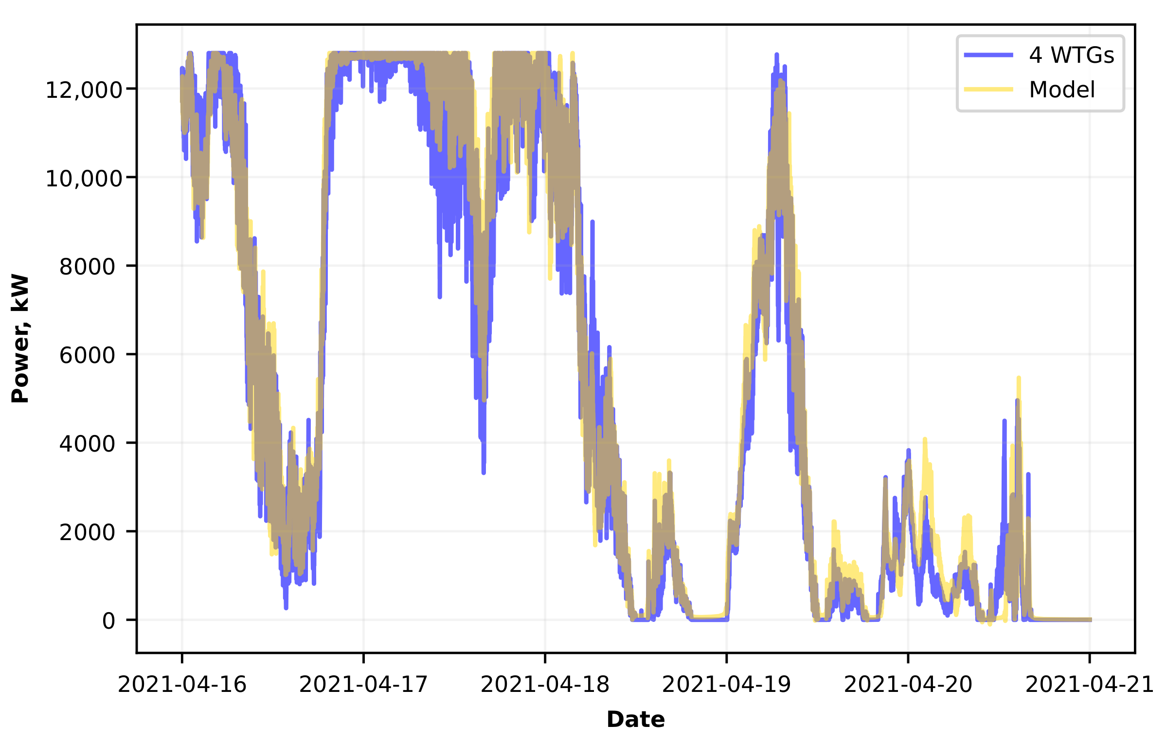
The proposed wind farm model introduced in previous subsections was inspected on a configuration with four aggregated WTGs with 3200 kW nominal power, while the representative WTG is selected from four WTGs. The amplitude parameter of the Gaussian random numbers for the surrogate method is 1 day (86,400 s), while $k=9$, meaning that the surrogate method is applied on the first nine scales and SEI-based model is used on the remaining scales. The power output of four aggregated WTGs and the proposed model are shown for the 5 day period on Figure 7.

The performance of the proposed model is validated against the primitive model, which obtains the power output of wind farm (or aggregated WTGs) by simply scaling the representative WTG power with the number of aggregated WTGs (four in the considered case). The model accuracy is quantitatively expressed using the power fluctuation magnitude ${\delta }_t^{WF}$, defined as the absolute power output difference between adjacent discrete intervals t and $t+\Delta t$, and normalized with installed capacity:

$${\delta }_t^{WF}=\left|{\displaystyle \frac{P_{t+\Delta t}^{WF}-P_t^{WF}}{N\times P_{nom}^{WTG}}}\right|,\forall t\in T,$$

(6)

where $P_t^{WF}$ and $P_{t+\Delta t}^{WF}$ are the power production of wind farm with N aggregated WTGs in discrete intervals t and $t+\Delta t$, respectively, and $P_{nom}^{WTG}$ is the nominal power of the WTG.

The comparison of the power fluctuations of four aggregated WTGs in wind farm, the proposed wind farm model, and a primitive model is depicted on Figure 8 for (a) 1 s resolution and (b) 1 min resolution data representing empirical histograms with 40 bins. It is evident that the primitive model cannot capture the power fluctuations accurately since higher frequency components are scaled linearly, which causes abrupt changes of power output that normally do not occur. This effect is present in both 1 s and 1 min resolution data. In contrast, the proposed WF model accurately preserves the power fluctuations.

The model in general accurately captures power fluctuations, but there may be periods with higher deviations caused by the complex winds on the analysed wind farm, resulting in significant deviations of the wind generation profile between WTGs. Higher deviations between the proposed model and actual power production of WF are expected to occur during periods with strong winds, where shut downs of multiple WTGs can occur, while the representative WTG shut down in general may not follow (or vice versa). As the model is based on a single WTG, the performance of the wind farm model is strongly dependent on the production profile of the WTG, requiring careful consideration of the representative WTG. However, during longer periods, short-term differences should not have a severe impact on the curtailment losses analysis.

3. Solar PV Farm Production Analysis

3.1. Solar Irradiance Measurements

The solar irradiance and air temperature measurements are collected from an Ammonit Meteo-40 data logger and include the whole year of 2021 sampled at 1 s resolution. The Delta-T SPN1 Sunshine Pyranometer is used for measurements of global horizontal irradiance (GHI) and diffuse horizontal irradiance (DHI).

The solar irradiance measurements are distanced approximately 125 km northwest from the analysed wind farm location. Even though solar and wind measurements were not taken at the same location, it is unlikely that it had an impact on the performed curtailment losses calculations in higher time resolutions for the following reasons:

• The location where measurements were taken exhibits very similar solar irradiance characteristics with wind farm location;
• Based on measurements in 56 wind farms and 12 solar irradiance stations across Sweden, Widen [29] showed that hourly correlations between combinations of wind farms and solar irradiance stations exhibit almost constant correlations in relation to the distance between wind farm and solar stations;
• Previous papers investigating complementarity between wind and solar resources found that the spatial correlations tend to decrease with the increase in time resolution [12,30].

3.2. Solar PV Farm Model

Since the solar PV farm power measurements were not available, the model is needed to convert the solar irradiance components (GHI, DHI) and other available parameters (air temperature, wind speed) to PV power production. This is a standard procedure during the wind farm expansion process. Considering that solar irradiance measurements are sampled at highly resolved resolution, typical solar PV performance models are not appropriate, i.e., they cannot capture the power fluctuations and the smoothing effect in PV farms. In this paper, the PV plant power model proposed by Marcos et al. [31] is implemented. The authors have found that the PV plant acts approximately as a first-order low-pass filter to solar irradiance fluctuations, causing the PV power production to be smoother than solar irradiance fluctuations measured by the pyranometer.

Moreover, they found that the smoothing effect in solar PV farms is proportional to the factor $\frac{1}{\sqrt{A}}$, where A is the area of the PV plant, and proposed the following transfer function (hypothetical filter) between the plane-of-array (POA) irradiance (input) and solar PV power (output):

$$H\left(s\right)=\frac{K}{{\displaystyle \frac{\sqrt{A}}{2\pi ·0.02}}\times s+1}.$$

(7)

Here, K represents the ratio of LV/MV transformer nominal power and irradiance at $G=1000{\mathrm{Wm}}^{-2}$. As seen from the equation, the hypothetical filter smoothing between the PV output power and the POA irradiance is only related to the area of the PV plant, while other factors contributing to the smoothing effect are not considered.

The PV plant topology considered in this paper assumes AC coupled system with fixed-tilt PV modules, DC cables, PV inverters, LV cables, LV/MV transformers, and MV cables. The PV plant does not share direct connections with the wind farm (e.g., via DC/DC converters) except for the MV cable connections at MV switchgear in MV/HV substation. In addition, the connections between the internal components of PV systems are not analysed in detail, but rather by their contributions to the system losses.

3.2.1. Solar PV Output Calculation Methodology

The model proposed by Marcos et al. [31] is modified and expanded to include the power losses and PV inverter clipping. The numerator of the Equation (7) is replaced with the ratio of PV plant installed capacity (instead of LV/MV transformer nominal power as originally used in [31]) and the irradiance $G=1000{\mathrm{Wm}}^{-2}$. In addition, the input to the hypothetical filter is POA irradiance corrected with the power losses in the PV plant before PV inverter (DC losses), as the transfer function itself cannot take into account the clipping effect of the PV inverter. Other effects such as PV module temperature changes should also be considered before applying the transfer function to prevent artificial fluctuations in AC power output.

Therefore, the total losses were decomposed into DC and AC losses, before and after the PV inverters. The transfer function defined in Equation (7) is used to convert POA irradiance, adjusted with compounded DC losses, to the input power of the PV inverters. Finally, PV farm output power is obtained after applying the inverter clipping and AC power losses. A more in-depth explanation of the losses is given in the Section 3.2.3.

The area of the PV plant is estimated from the PV plant installed capacity by using the ratio of 1 MWp/Ha.

3.2.2. POA Irradiance Calculation

As the input variable in the solar PV plant model is POA irradiance, measured GHI and DHI from the pyranometer have to be converted to global POA irradiance. In the intermediate step, direct normal irradiance (DNI) is calculated from GHI and DHI measurements.

Python pvlib package [32] is used to convert 1 s solar irradiance components to global POA irradiance at the PV modules with the use of isotropic sky diffuse model. A fixed-tilt south-oriented PV system is assumed with the surface tilt angle of 20°.

3.2.3. Power Losses in the Solar PV Farm

The detailed power losses in the PV plant are represented in

Table 1. Detailed solar PV system losses (not including PV module temperature and clipping losses).

PV Losses	Percentage
Soiling	2.0%
Shading	2.0%
Mismatch	1.5%
LID	1.0%
DC wiring	1.5%
Inverter	1.5%
AC wiring	0.5%
LV/MV transformer	0.5%
MV line	0.5%

. This does not include temperature losses in PV modules and PV inverter clipping losses which are separately taken into account. Temperature losses due to PV module heating are modelled in python pvlib package using the Faiman empirical heat loss model [33], which calculates PV module temperature by considering the POA global irradiance, air temperature, and wind speed at the PV module height. Air temperature measurements are taken from the pyranometer, while wind speed at the module height is calculated from available wind speed measurements from one of the WTGs at the nacelle, using the well-known Hellmann exponential law:

$$v_t^{mod}=v_t^{WTG}\times {\left({\displaystyle \frac{H^{mod}}{H^{WTG}}}\right)}^{\gamma },\forall t\in T,$$

(8)

where $v_t^{mod}$ is the wind speed at the PV module height $H^{mod}$, $v_t^{WTG}$ is the wind speed measured at the nacelle with height $H^{WTG}$, and $\gamma$ is the Hellman exponent. The value of $\gamma$ = 1/7 is used for Hellman exponent [34].

The effect of temperature on PV module efficiency is accounted by using PV module temperature factor, calculated using the following equation:

$$f_t^T=1+{\theta }_T\times (T_t^{mod}-25°C),\forall t\in T$$

(9)

where ${\theta }_T$ is the PV module temperature coefficient of power and $T_t^{mod}$ is the PV module temperature calculated from Faiman empirical loss model. The PV modules with ${\theta }_T=-0.42$ $\%/°\mathrm{C}$ are used. The temperature factor $f_t^T$, $\forall t\in T$, is adjusted with the DC losses (due to soiling, shading, mismatch, LID, DC wiring as represented in Table 1) in PV system according to Equation (10) to obtain total DC losses before PV inverter clipping.

$$\begin{array}{c}\hfill L_t^{dc}=1-f_t^T\times \prod _i\left(1-\frac{l_i^{dc}(\%)}{100}\right),\forall t\in T.\end{array}$$

(10)

The POA irradiance, corrected with the DC losses represented in Equation (10), is used as an input to hypothetical filter represented in Equation (7). The output of the hypothetical filter represents an input power to the PV inverters $P_t^{inv,in}$.

PV inverter clipping losses occur during periods when PV module production is higher than PV inverter nominal power. This is caused primarily due to the ratio of the PV module capacity to inverter nominal power, also known as DC:AC ratio or inverter loading ratio, being above 1.0. Underdimensioning PV inverter nominal power boosts project economics, allowing the AC power production to have longer periods with maximum power and compensates for PV module degradation over project lifetime [35]. A DC:AC ratio of 1.1 is utilised throughout this paper. Although large-scale PV plants contain multiple PV inverters, for simplicity reasons, the PV plant is modelled as having a single PV inverter with nominal power $P^{inv,nom}$ given by the ratio of PV installed capacity and inverter loading ratio. However, the used procedure essentially outputs the same results as using multiple PV inverters with DC power split equally among inverters.

Given the nominal power of the inverter $P^{inv,nom}$, the output power of the PV inverter for each $t\in T$ is given as:

$$\begin{array}{cc}\hfill P_t^{inv,out}=& \left\{\begin{array}{c}{P}^{inv,nom}\mathrm{if}{P}_t^{inv,in}\ge P^{inv,nom}.\hfill \\ P_t^{inv,in},\mathrm{otherwise}.\hfill \end{array}\right.\hfill \end{array}$$

(11)

Lastly, the output power of the solar PV farm, $P_t^{PV}$, corresponds to the $P_t^{inv,out}$ adjusted with total AC losses in the PV farm calculated as follows:

$$\begin{array}{c}\hfill L_t^{ac}=1-\prod _i\left(1-\frac{l_i^{ac}(\%)}{100}\right),\forall t\in T,\end{array}$$

(12)

where $l_i^{ac}(\%)$ represents individual AC losses (Inverter, AC wiring, LV/MV transformer, and MV line).

It is important to stress that clipping losses in PV inverters also depend on the time resolution [36]. The additional clipping losses (difference between losses in higher and lower resolutions) can be included in curtailment losses. However, additional clipping losses as a result of inverter operation are not the focus of this paper and are not considered.

4. Curtailment Losses Calculation

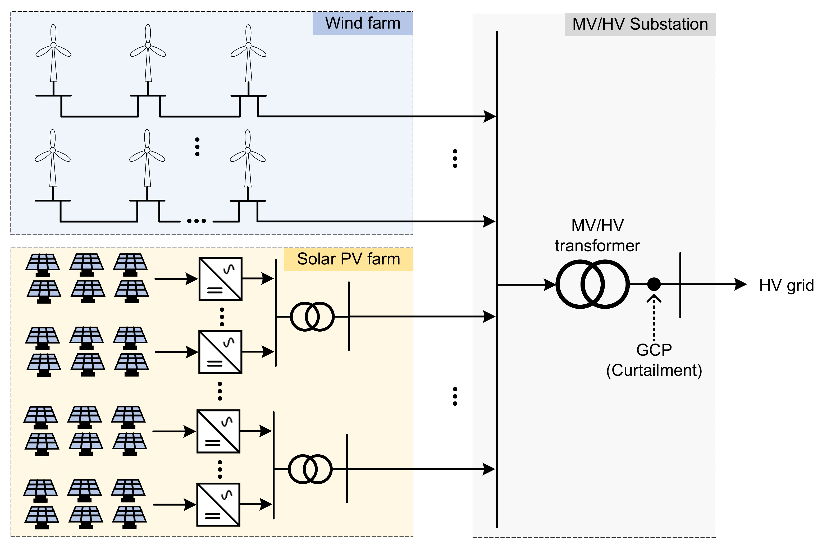
As wind farm and solar PV farm power production time series in high temporal resolution are available, methodology for curtailment losses calculation is introduced. The output power of wind and PV farm is evacuated through a respective MV switchgear and MV/HV transformer to the grid. The structure of the hybrid wind–PV system is depicted on Figure 9. The grid connection point (GCP) where power is curtailed is located at the HV side of the MV/HV transformer. Therefore, the calculation of MV/HV transformer losses, common to both wind and solar PV farms, is a prerequisite before curtailment calculation.

The HPP control system considered in this paper has simple curtailment logic: whenever the aggregated WF and PV power production is above the grid cut-off power ($P^{max}$), the power is curtailed to exactly $P^{max}$. The power curtailment occurs temporarily.

4.1. MV/HV Transformer Losses

The MV/HV transformer losses are divided into variable and no-load losses:

$$\Delta P_t^{TR}=P_c·{\left({\displaystyle \frac{S_t^{HPP}}{S^{nom}}}\right)}^2+P_0,\forall t\in T,$$

(13)

where $P_c$ are nominal copper losses, $S_t^{HPP}$ is the apparent power of the HPP at given timestamp t, $S^{nom}$ is the MV/HV transformer nominal power, and $P_0$ represents no-load losses in transformer. The reactive power passing through the transformer is not considered, hence active power is used instead of apparent power, such that $S_t^{HPP}=P_t^{WF}+P_t^{PV}$.

Since wind and solar PV farms with various installed capacities are examined, a simple estimation of the transformer parameter in Equation (13) is used. Transformer nominal power is estimated to have a value 10% higher than grid cut-off power, while nominal copper losses are 0.1% of the nominal power, and no-load losses are 20% of the copper losses. While this is a rough estimation of the transformer parameter, it serves to automate the process of calculations and has minimal impact on the curtailment losses.

4.2. Method of Calculation for Different Time Resolutions

Wind and solar power time series available in 1 s resolution are used as a base to form several other time resolutions: 2 s, 5 s, 10 s, 30 s, 1 min, 2 min, 5 min, 10 min, 15 min, 30 min, and 1 h. To allow calculations of curtailment losses when wind and solar PV power time series have different time resolutions, e.g., 10 min wind farm and 1 h solar power time resolution, a special procedure is proposed. Namely, 1 s wind and solar power time series are downsampled to the above-mentioned resolutions, separately for wind and solar power time series, by averaging the given time interval. Downsampled averaged time series are then upsampled back to 1 s resolution using the forward-fill method (missing values in the given interval are filled with the closest available value at the start of the interval). After accounting for losses in MV/HV transformer, the HPP production is obtained as the sum of the wind and solar power production time series. Summation is allowed as the downsampled averaged data are upsampled back to 1 s resolution.

For the purpose of this paper, the curtailment losses are defined as energy losses, represented as the sum of power curtailment occurring whenever potential HPP production exceeds the grid connection capacity, expressed in absolute values (e.g., MWh) or percentage of potential HPP production (i.e., before curtailment). The power curtailment at the GCP is calculated as follows:

$$\begin{array}{cc}\hfill \Delta P_t^{curt}=& \left\{\begin{array}{c}{P}_t^{WF}+P_t^{PV}-\Delta P_t^{TR}-P^{max},\mathrm{if}{P}_t^{WF}+P_t^{PV}-\Delta P_t^{TR}\ge P^{max},\hfill \\ 0,\mathrm{otherwise},\hfill \end{array}\right.\hfill \end{array}$$

(14)

where $P_t^{WF}$ and $P_t^{PV}$ are output power of the wind and solar PV farm model at time interval t, before MV/HV transformer losses, respectively. The curtailment losses (in absolute values) are calculated as:

$$\Delta E^{curt}=\Delta t\times \sum _{t\in T}\Delta P_t^{curt},$$

(15)

where $\Delta t=1/3600\mathrm{h}$ is time step for 1 s data. Therefore, the curtailment losses in percentage values correspond to:

$$\Delta E_{\%}^{curt}={\displaystyle \frac{\Delta E^{curt}}{{\sum }_{t=1}^T\left(P_t^{WF}+P_t^{PV}-\Delta P_t^{TR}\right)\times \Delta t}}.$$

(16)

Curtailment losses can be also expressed in % of energy produced by a single technology, e.g., PV. In such cases, the denominator of Equation (16) is replaced with the PV production.

5. Results

The curtailment losses in different time resolutions are influenced by many factors which are separately investigated. Curtailment losses are calculated by inspecting the effect of: (1) various seasons by grouping the data into two- or three-month periods and analysing separately (Section 5.1); (2) grid cut-off power in relation to HPP capacity (Section 5.2); (3) wind and solar PV installed capacity (Section 5.3); (4) unequal proportion of wind and solar PV capacity in HPP, i.e., the specific case when an existing wind farm is hybridized with solar PV farm having different installed capacities (Section 5.4).

5.1. Curtailment Losses for Different Time Resolutions and Seasonal Effect

As wind and solar production are dependent on underlying resource variation, seasonal changes will also affect power fluctuations. Curtailment losses during specific periods will depend on the number of instances in which cumulative wind and solar PV power were near or above the grid cut-off power. To reduce the impact of a single or few occurrences of higher HPP production on the results, curtailment losses should be analysed for at least a monthly period. The wind and solar power time series are grouped into winter (January and February), spring (March, April, and May), and summer (June, July, August) months and analysed separately. The autumn months are also analysed, but not shown, as the results did not show significant differences to spring and winter with the respect to additional curtailment losses.

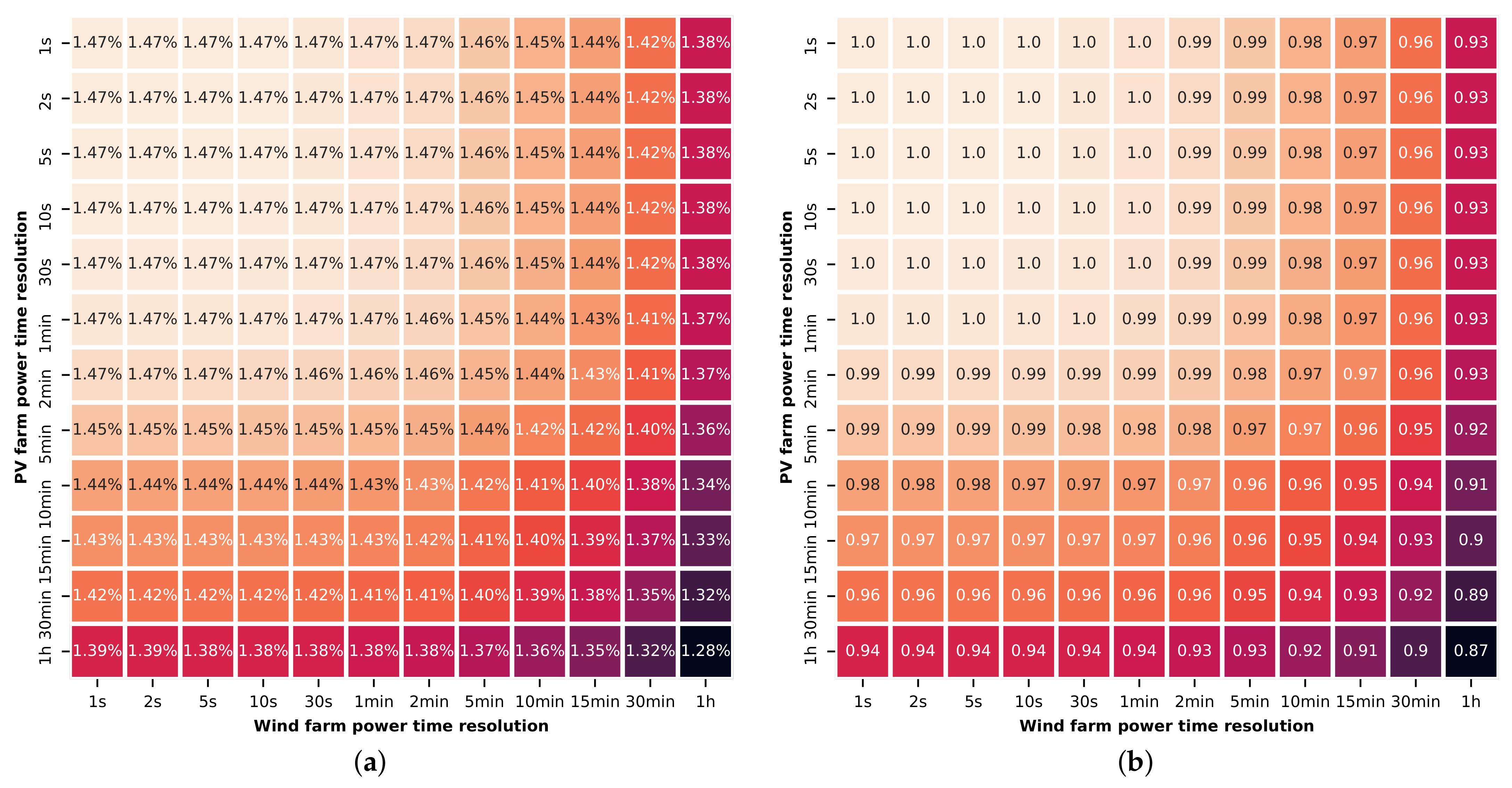
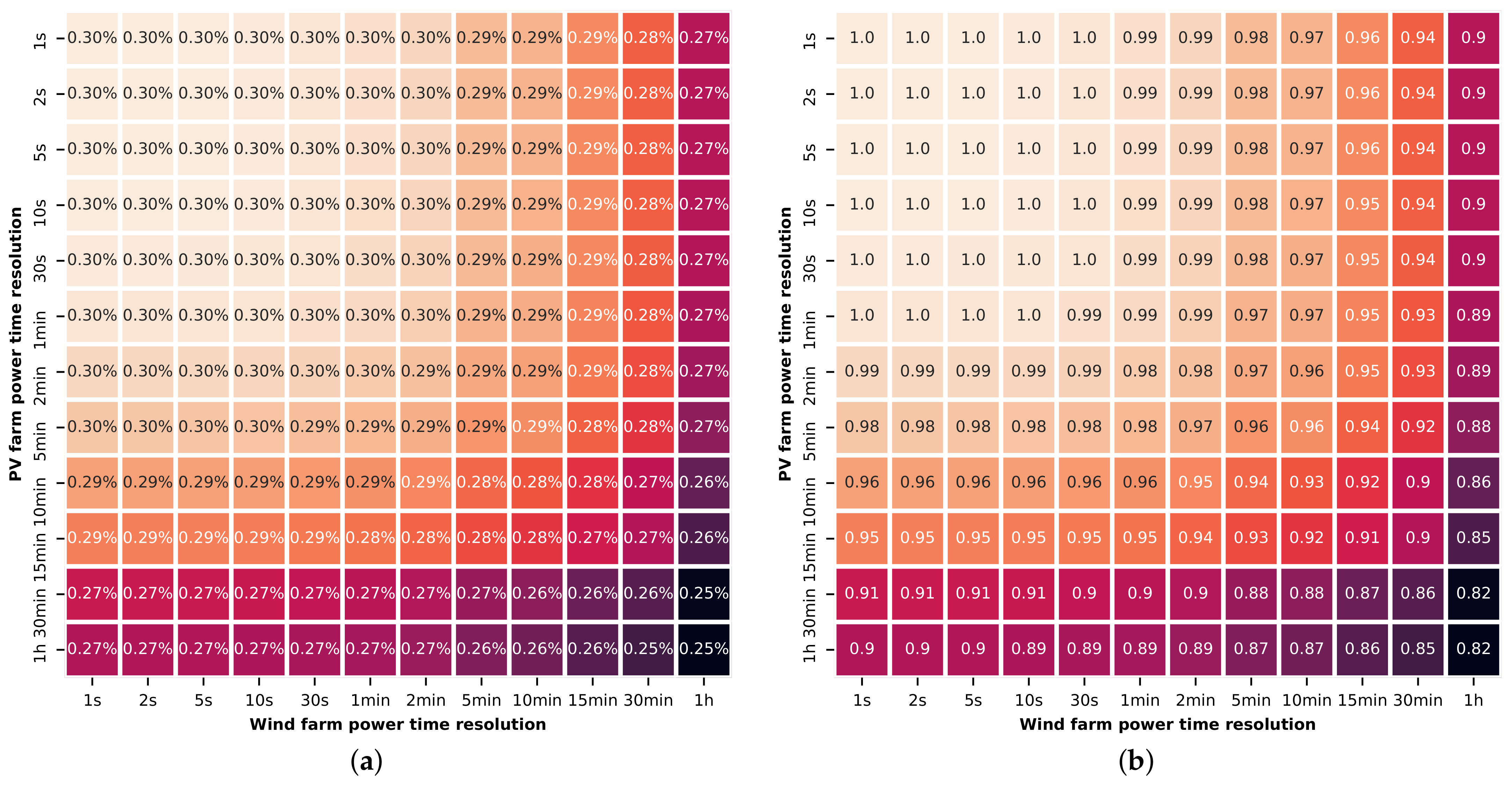
As a starting point for the analysis, wind and solar PV plants with installed capacity 25.6 MW/25.6 MWp are used. The grid cut-off power is designated to 70% of the HPP capacity ($0.7·51.2$ MW $=35.7$ MW). The curtailment losses for winter, spring, and summer months are represented in Figure 10, Figure 11 and Figure 12, respectively. The curtailment losses are represented as heatmaps, with wind farm power time resolutions in columns and solar PV power time resolutions in rows. On each figure, curtailment losses are represented in (a) percentages of potential HPP energy production at the GCP before curtailment and (b) relative values of curtailment losses versus 1 s resolution (for easier comparison). For example, the 1 h resolution for wind and solar PV power in Figure 10 results in 82% of the losses captured in 1 s resolution.

It can be seen that curtailment losses are almost identical for time resolutions between 1 s and 1 min. In other words, using time resolution below 1 min does not reveal additional curtailment losses compared to 1 s for HPPs with comparable or larger capacities. Furthermore, by looking at the curtailment losses in the upper triangle (higher solar PV compared to wind power time resolution) and lower triangle of the curtailment losses matrix (higher wind resolution), it can be stated that wind and solar PV power fluctuations have contributed somewhat equally to additional curtailment losses. In reality, this can vary depending on the wind and solar PV farm size and local variations of solar irradiance and wind speed (especially for smaller-scale HPPs). A comparison of the curtailment losses for winter, spring, and summer shows that significant deviations of percentage curtailment losses can occur seasonally, but with similar relative changes between different time resolutions.

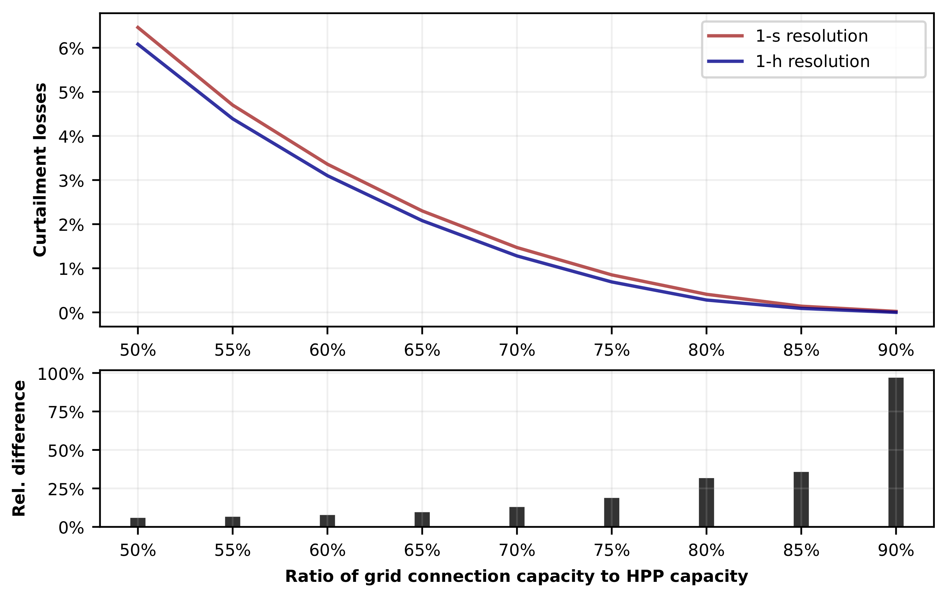
5.2. Effect of Grid Cut-Off Power

The impact of grid cut-off power on curtailment losses was investigated for the spring months and 25.6 MW/25.6 MWp wind and solar PV capacity. The ratio of grid cut-off power ($P^{max}$) to HPP installed capacity ($P^{HPP}$) varied within range of 50% to 90% with 5% step, as depicted in Figure 13. The comparison of curtailment losses is provided in the 1 h versus 1 s resolution of wind and solar PV power time series, as a function of $P^{max}/P^{HPP}$ ratio. Curtailment losses are depicted percentage-wise and as relative percentage differences.

In the case of $P^{max}=70\%P^{HPP}$, curtailment losses captured in 1 s resolution are 1.47%, while losses are 1.28% for 1 h resolution, resulting in 12.9% underestimation of actual curtailment losses (curtailment losses calculated in 1 s resolution can be referred to as actual losses) when 1 h resolution is used. Increase in $P^{max}/P^{HPP}$ ratio to, e.g., 85% leads to 0.14% and 0.09% curtailment losses in 1 s and 1 h resolution, respectively, which results in 35.7% underestimation. In contrast, for $P^{max}=50\%P^{HPP}$ curtailment losses will be 6.46% and 6.08% in 1 s and 1 h resolution, respectively, leading to only 5.9% underestimation.

Therefore, when grid cut-off power is increased relative to HPP capacity, curtailment losses are reduced, but relative additional curtailment losses calculated in different resolutions will increase. This is anticipated as there is a lower probability that, during a given discrete time step wind and solar PV power, in both higher and lower resolution, will simultaneously reach grid cut-off power of, e.g., $P^{max}=70\%P^{HPP}$ than $P^{max}=50\%P^{HPP}$. Therefore, higher underestimation occurs when total curtailment losses are lower.

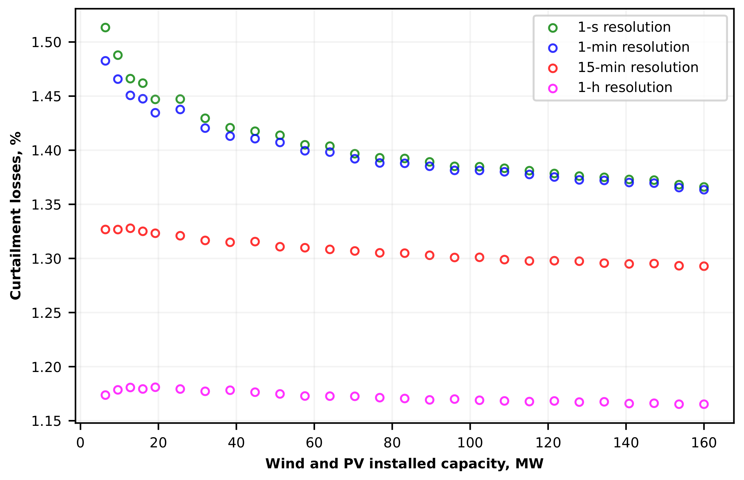
5.3. Effect of Wind and Solar PV Size

An important aspect to consider is wind and solar PV farm installed capacity. Previous calculations are provided only for wind and PV capacities of 25.6 MW/25.6 MWp. Higher installed capacities will reduce power fluctuations due to the smoothing effect and therefore reduce the relative difference between curtailment losses at different resolutions, and vice versa.

Using a 3.2 MW WTG as the base of the wind farm model, wind power time series are generated as multiples of WTG nominal power, starting from two WTGs (6.4 MW) up to 50 WTGs (160 MW). The computational burden was decreased by skipping every odd number of WTGs after the first six WTGs. The modelled PV installed capacity in every simulation is equal to the sum of the WTGs nominal power (equal proportion of wind and solar capacity in HPP). The analysis is provided by using the wind and solar data from April 2021, while grid cut-off power is 70% of HPP installed capacity. Although April is not representative of the whole year, it emphasizes the prospective additional curtailment losses during periods with higher fluctuations.

The curtailment losses for different wind and solar sizes are represented in Figure 14 and compared for 1 s, 1 min, 15 min, and 1 h time resolution. It is observable that additional curtailment losses are in general reducing with the increase in wind and solar PV capacity. Curtailment losses calculated in 1 s and 1 min resolution show a strong rise for lower wind and solar capacities, in contrast to losses calculated in 15 min and 1 h resolutions. Indeed, in both 15 min and 1 h resolutions, differences in curtailment losses are practically not observable with the change in installed capacity of wind and solar PV plants. This is explained by the fact that the smoothing effect is not as significant in lower resolutions.

Nonetheless, for installed capacities of wind and solar below 10 MW/10 MWp, a sharp increase of additional curtailment losses can be expected. This can result in the higher underestimation of curtailment losses for HPPs with lower installed capacities when low resolutions are utilised. For HPP with wind and solar farms having 6.4 MW/6.4 MWp capacity, actual curtailment losses are 28% higher than captured in 1 h resolution and 14% higher than captured in 15 min resolution. In contrast, significant deviations between 1 min resolution and 1 s resolution are not obvious.

5.4. Hybridization of the Existing Wind Farm

In all previously analysed scenarios, wind and solar PV capacity had equal capacity shares in HPP (50% wind and 50% solar). An interesting and widespread business case for utilisation of HPPs is the hybridization (expansion) of existing wind farms with solar PV farms, without increasing the grid connection capacity. The opposite is also possible (i.e., expansion of existing solar farm with wind capacity), but less common in practical applications.

In the analysed case, the power at the GCP is already limited to the wind farm installed capacity. More precisely, the grid cut-off power at the GCP is often slightly lower than wind farm capacity to improve economics of the wind farm. For simplification purposes, it is assumed that the grid cut-off power is equal to the wind farm capacity, i.e., $P^{max}=P^{WF}$. A wind farm with 10 WTGs and 3.2 MW nominal power each is analysed. The solar PV installed capacity is varied between 1 MWp and 32 MWp to analyse the impact of the solar PV farm size. The analysis is provided for February, April, and July. The additional variable losses in MV/HV transformer, caused by the PV production, are not considered.

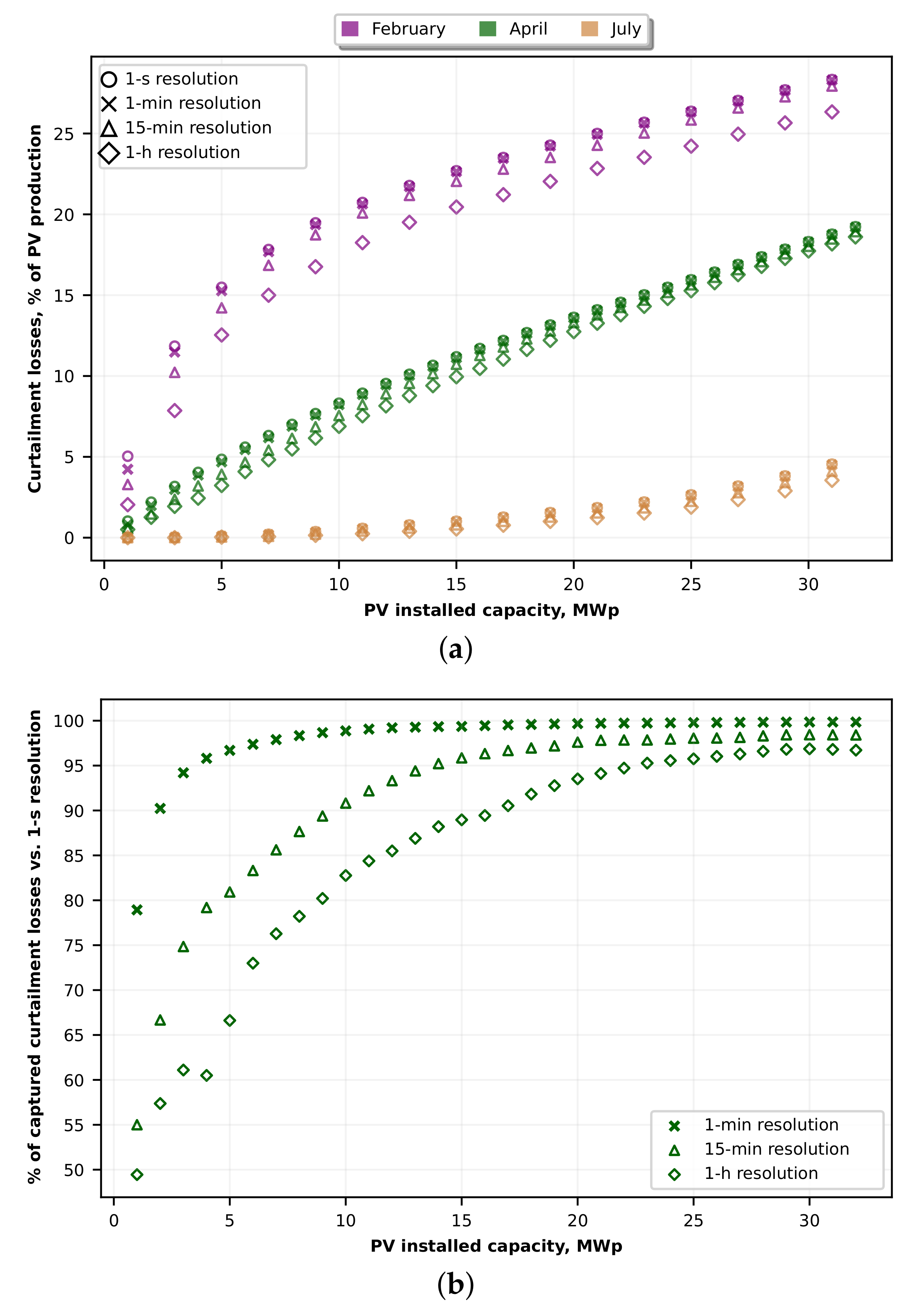
Before hybridization, curtailment losses were zero since grid connection capacity is equal to the wind farm installed capacity. Hence, when a wind farm is expanded with a solar farm, curtailment losses will be assigned to the solar PV plant. On Figure 15, the curtailment losses results are represented when the existing wind farm with 32 MW is expanded with a solar PV farm with capacities between 1–32 MWp (step is 1 MWp). The results are shown as (a) % of PV production for the February, April, and July and (b) curtailment losses in 1 min, 15 min, and 1 h resolution as a percentage of losses in 1 s resolution for the April. The trend of increase in curtailment losses is changing over different months, but overall the additional curtailment losses percentage-wise are decreasing with additional solar PV capacity added, as clearly shown in Figure 15b.

It can be seen that additional curtailment losses in higher resolutions can be significant when PV installed capacity is lower than 10 MWp. In the case of April, when the wind farm is expanded with a solar PV farm with 1 MWp capacity, only 50% of the actual curtailment losses can be captured using 1 h resolution. This is somewhat in line with previous results in Section 5.3, if the losses for 6.4 MW/6.4 MWp HPP are to be extrapolated in the direction of lower capacities. In terms of the percentage of solar production, it corresponds to approx. 1% in 1 s resolution versus 0.5% captured in 1 h resolution.

For a 5 MWp PV plant, percentage-wise this is an increase from 3.2% in 1 h resolution to 4.8% in 1 s resolution. In contrast, curtailment losses captured with 1 min resolution are 79% for April and 84% for February in comparison to 1 s resolution. In the case of 1 MWp solar PV farm, during February curtailment losses captured in 15 min resolution were roughly 50% of the 1 s curtailment losses, indicating that higher time resolution may be needed when curtailment losses are evaluated for smaller-scale PV plants.

After the solar PV capacity reaches 25 MWp, the saturation effect in 1 h resolution becomes apparent, and unit change in PV capacity does not significantly affect the additional captured losses in 1 h resolution. The higher the time resolution, the saturation effect will start earlier (e.g., approx. 5 MWp for 1 min and 15 MWp for 15 min resolution).

6. Discussion

Time resolution used for power time series of large-scale hybrid wind–PV farms has an important impact on estimation of curtailment losses as the use of lower resolutions flattens the power peaks occurring in shorter time frames. Current publications related to calculations of curtailment losses in hybrid wind–PV farms have either used low time resolutions (most frequently 1 h averages), or higher, but without comparative analysis between different resolutions. While the calculations of curtailment losses in lower time resolutions are relatively simple due to availability of classical wind and solar power performance models, the main obstacle in providing calculations in higher time resolutions is taking into consideration the smoothing effect. The latter requires the use of specialized wind and solar PV power production models that can effectively scale the power without introducing artificial power fluctuations. This paper provided curtailment losses calculations in highly resolved time resolutions and comparison with lower time resolutions typically used for curtailment losses analysis, while accounting for wind and solar PV smoothing effect with the use of specialized models.

The findings of this paper suggest that 15 min resolution provides an accurate estimate of curtailment losses in large-scale hybrid wind–PV plants, and it is generally preferred over 1 h resolution when more accurate curtailment estimation is required. The use of 1 min time resolution can additionally improve the curtailment losses estimation accuracy over 15 min resolution, but the improvement is not significant for wind/solar PV plants with installed capacity above 10 MW/10 MWp. In addition, the use of sub-minute time resolutions has no further effect compared to 1 min time resolution for large-scale wind–PV farms.

The considered time resolution for curtailment estimation studies should be tackled in conjunction with installed capacity (size) of wind and PV farms. For wind and PV installed capacities above approximately 25 MW/25 MWp, saturation in smoothing effect becomes evident, as additional WTGs or unit area of PV modules results in smaller reduction of power fluctuations and, indirectly, the curtailment losses. Thus, a significant reduction in power-peak flattening and additional curtailment losses is not expected for, e.g., 200 MW/200 MWp versus 50 MW/50 MWp HPPs, indicating that 15 min resolution may still be recommended over 1 h resolution for very large-scale HPPs. However, more attention should be given to hybrid wind–PV plants with capacity below 10 MW/10 MWp. Results indicate that in such scenarios 15 min or 1 h resolutions do not provide accurate estimates and that 1 min resolution may be required. A detailed analysis of curtailment losses for smaller hybrid wind–solar PV sizes is out of the scope of this paper. Nonetheless, future considerations regarding smaller-scale HPPs may not be important as wind turbine manufacturers continue to increase the nominal power ratings of WTGs, with mainstream WTGs as of today already having 5–7 MW of rated power [37], while smaller WTGs are practically going out of production.

The detailed recommendations on the time resolutions for curtailment evaluation studies have not yet been adequately addressed and justified in the literature. Previous reports instructing the use of 10 min or 15 min resolution for curtailment evaluation studies proposed in [5,19] has not considered wind and solar PV capacity, which have a major role, as shown in this paper. These recommendations are acceptable and in accordance with the results of this paper for HPPs having installed capacities above approximately 10 MW/10 MWp. In the case of HPPs with installed capacity significantly above 10 MW/10 MWp, planners can also utilise a 1 h time resolution for wind and solar PV power production time series if 10 min or 15 min data are not available. Certain underestimation of curtailment losses will be expected, but calculations should provide reasonable estimates.

The ratio of grid cut-off power and HPP installed capacity is an important aspect during the planning and design process, as low ratio values can result in excessive curtailment losses. However, the ratio has reverse effect on additional curtailment losses. Namely, when the ratio is, e.g., 90%, the additional curtailment losses captured in higher resolutions will increase compared to the 70% case, but at the same time the curtailment losses will be relatively small. Therefore, the impact of additional increase of curtailment losses may be irrelevant. In contrast, lowering the ratio to, e.g., 50% may increase the curtailment losses to relatively high values, but additional losses captured in higher resolutions will decrease compared to the 70% case.

In the case of wind farm hybridization, the possibility of increasing the grid connection capacity (closely tied to the wind farm capacity) may not be possible, economically feasible, or achievable within a reasonable time. Therefore, in most cases it will not be justifiable to install the same PV capacity as the wind farm (unless high anti-correlation is observed on site), but rather a smaller portion of wind capacity. If the wind farm constrains the PV farm to smaller capacities (e.g., below 10 MWp), higher underestimation of curtailment losses may occur when lower time resolutions are used.

Finally, the limitations of this paper are emphasized. The analysed WTGs have a nominal power rating of 3200 kW and double-fed induction generators. It is not known how the smoothing effect characteristics of newer-type wind turbines will change (e.g., by comparing the smoothing effect in wind farms with x analysed WTGs and y newer-type WTGs, with the same installed capacity). The PV plant model as a first-order low-pass filter for POA irradiance based on Marcos et al. [31] assumes that the only relevant factor for the power fluctuation smoothing is the area of the PV plant. However, the power fluctuations of the PV plants also depend on the cloud speed [38] and the layout of the PV plant itself [39]. Furthermore, the model does not consider the effects of PV inverters [40], panel configuration (fixed-tilt, single-axis or dual-axis) [41], and other factors contributing to the potential reduction in power fluctuations. Lastly, the conclusions derived from this paper are applicable only if HPP control system curtails power above grid cut-off power instantaneously. In case certain power limitation flexibility is allowed, e.g., possibility of short-term excess power by limiting the 15 min average power of HPP (billing period) to grid cut-off power, curtailment losses calculation in time resolutions shorter than 15 min would not need consideration.

7. Conclusions

In this paper, the impact of time resolution of wind and PV power production on curtailment losses in large-scale hybrid wind–PV farms is examined. Specialized scalable wind and solar PV power models are used to produce power output in 1 s resolution while accurately preserving power spectrum, allowing the analysis of wind and PV size impact on the curtailment losses. Highly resolved 1 s output power was resampled, providing the comparison of curtailment losses in different time resolutions. Additionally, the impact of grid cut-off power and different shares of wind and solar PV capacity on curtailment losses is also considered.

The major findings can be emphasized as follows:

• Appropriate time resolution for accurate estimation of curtailment losses in hybrid wind-PV plants cannot be predefined without considering the wind and solar PV plant installed capacity (size);
• 15 min resolution is generally preferred over 1 h resolution for large-scale hybrid wind-PV plants if more accurate assessment of curtailment losses is required;
• 1 min resolution can additionally improve the estimation of curtailment losses over 15 min resolution, but the improvement is not significant for wind and PV plants with capacity above approximately 10 MW/10 MWp;
• The time resolutions higher than 1 min (i.e., intra-minute resolution) do not offer improved estimation of curtailment losses over 1 min resolution for large-scale hybrid wind-PV plants;
• The possibility of higher underestimation of curtailment losses can occur in HPPs with wind/PV capacity below approximately 10 MW/10 MWp if low time resolutions are utilised (15 min, and particularly 1h).

Although the curtailment losses in HPPs primarily depend on local wind speed and solar irradiance complementarity and thus require individual treatment, the local complementarity is not the driving force that effects the additional curtailment losses estimated in higher temporal resolutions, as the mutual dependence between the variations of the wind and solar irradiance weakens with the increase in temporal resolution. The influence of high-frequency wind and irradiance fluctuations on power output of large-scale wind and solar PV plants is additionally limited due to strong smoothing effects, which allows for better generalization of the major findings and their applicability to other locations. However, the 10 MW/10 MWp power threshold should not be considered stiff, but rather an approximate or indicative value that will also depend on external influences to some extent, such as meteorological conditions. While it is expected that the influence of site-specific meteorological conditions on additional curtailment losses in large-scale wind-PV HPPs will be limited, the further research is required to evaluate its quantitative effects.