Abstract
The fast frequency response (FFR) function in renewable energy source (RES)-based power stations has proved to be able to improve the frequency stability of power systems with high RES penetration significantly. However, most current FFR functions in photovoltaic (PV) power stations typically show power response deviations and unnecessary power loss issues that are caused by inadequate station power distribution strategies. This is particularly important in cases where the power must be increased when the system frequency shows a downward disturbance. This paper proposes a new distribution strategy for FFR in PV power stations and studies related distribution strategies, system structures, calculation algorithms, function execution effect, and active power regulation technology. The proposed approach uses a proportional distribution strategy based on an evaluation of the real-time potential maximum power capability values of the subarrays or generation regions, which are evaluated using a few reference inverters located in every subarray or region. Real-site deployments and tests have been completed in PV power stations to verify the effectiveness of this new distribution strategy, and the proposed FFR solution using this distribution strategy has demonstrated strong performance and potential for wider application scenarios.
1. Introduction
Because of worldwide environmental deterioration and the fossil fuel-based energy crisis, many countries have declared goals for net zero carbon emissions [1,2,3]. Upon declaration of the targets of peak carbon emission by 2030 and carbon neutralization by 2060, large numbers of renewable energy sources (RESs) have been installed in China, including wind power and photovoltaic power sources [4]. The high penetration of RESs into power systems and the reduced use of traditional thermal or hydrogen power plants have led to an obvious decline in system inertia [4,5,6]. The challenges associated with RES integration into the system’s frequency response, and the ways in which these challenges affect system reliability, have been reviewed in [7]. The fast frequency response (FFR) service is a regulated power resource/product designed for rapid changes in the short-term frequency caused by insufficient synchronization inertia in the power system. FFR is mainly generated by asynchronous power resources (e.g., photovoltaic, electrochemical battery energy storage, wind power, and fast adjustable loads) through inverters or relays. Using a combination of rapid power injection and a synchronous inertia response, FFR can prevent rapid frequency change from occurring within a short time after a disturbance. This provides time to start up the primary frequency regulation mechanisms of thermal/hydro power and other inertia generator units based on governors in order to maintain the power system’s frequency stability.
Studies [8,9] have shown that RES systems with slow response capabilities have a significant negative impact on power system frequency security. To address this issue, RES stations equipped with FFR technology, with response times ranging from several hundred milliseconds to several seconds, are required to enhance the power system’s frequency robustness and maintain system stability [1,4,5,6]. To evaluate and make the best use of the FFR capability of the target power system, there are two main challenges: they involve determining the potential maximum power capability (PMPC) value of the power system and finding an efficient strategy for power distribution between the generation units. The PMPC value of a photovoltaic (PV) power system represents the maximum available PV power headroom of the PV at a specific time, regardless of whether the power is actually being produced, e.g., during a power-limited state. Relevant factors involved in the PMPC include the status of the power inverter/converter equipment, the solar radiation, the ambient temperature and humidity, the PV panel inclination, the wind speed, and the dust coverage.
Although the FFR control system architecture in most PV power stations physically contains three-layer architecture (i.e., station, subarray, inverter), logically it may contain either two layers (station direct to inverter) or three layers (station, subarray data logger, inverter), which represent different distribution strategies. Existing research on FFR technology has rarely investigated the impact of intra-station power distribution on FFR, and the shortcomings of the current power distribution strategies in FFR projects for PV stations are usually ignored.
At present, a large number of the FFR projects in PV stations in China have been verified by performing on-site testing [8,9,10,11]. However, they still show some deficiencies in terms of full utilization of the PMPC of the PV station. Although the PMPC value of the PV station is sufficient to meet the regulation power target requirements during the FFR process, the regulation method still involves a certain probability of unnecessary power abandonment. In particular, this can occur when the power station is operating in a limited power state and is then expected to increase power during a downward frequency disturbance without using a battery energy storage.
Numerous studies have been published in the literature with regard to power distribution strategies for PV power generation. The control strategies in these articles can be roughly divided into two categories [12,13]. The first strategy type requires each single inverter to participate actively in power regulation based on its own power response characteristics during a frequency disturbance [13,14,15,16]. In [13], an active power generation method based on PV virtual synchronous inertia control technology was proposed. However, the algorithm was complex and would be difficult to commercialize in engineering terms. A power generation control strategy based on the quadratic interpolation method, with consideration of the Lagrange algorithm, was proposed in [14,15]. However, the convergence and sharpness of this strategy remain dubious and require further study, especially under circumstances in which the external environment of the inverter or the PV module changes. A PV power distribution method that considered the load shedding rate of a single inverter was proposed in [17]. This strategy requires an advanced algorithm to perform accurate calculations and power allocation for the single inverter in the power system [18]. The algorithms above, based on independent execution of a single inverter, have mainly been used in small PV power systems with one or only a few inverters. However, they have not been used in PV power stations and thus will not be discussed in further detail in this paper.
The second strategy is the power response method, based on the power order from the superior station-level power control system [19]. This strategy is the dominant power control method used in large- and medium-sized PV power stations, with control systems that contain an automatic generation control (AGC) system, an FFR control system, or a power plant controller (PPC) [20,21,22]. In [20], a rated capacity-based coordinated distribution strategy for PV stations was proposed for use under various response speed conditions. Reference [21] presents an average strategy-based solution for AGC systems that allocates power to each PV inverter by determining the power distribution range and the active power margin. In [22], the start-up and turn-off sequences of inverters with different rated capacity types were allocated to improve the accuracy of the grid dispatching instructions, as well as the equipment lifetime of large PV power stations. The following three power distribution strategies for PV station control systems were summarized in [23,24]: (1) an average distribution strategy with respect to each individual inverter, (2) a proportional distribution strategy based on the maximum capability of each inverter, and (3) a cyclic sleep distribution strategy. The first strategy is used more frequently than the other two methods. For the second strategy, however, no feasible method was proposed for the evaluation of the real-time PMPC value of a single inverter, particularly when the inverter is in the limited power state. Therefore, the second strategy mentioned in this article is simply a virtual but impractical distribution concept. The third strategy is rarely used in real PV projects because of its ignorance of the main focus [24].
All the station control methods above fail to solve the FFR power response deviation problem and the unnecessary power loss problems in PV power stations. This paper proposes a new distribution strategy and studies the internal power distribution strategies used between subarrays inside PV power stations for the FFR control system. A new station distribution strategy is proposed, based on the evaluated real-time PMCP value of each subarray. In on-site testing, the effectiveness of the proposed new method is verified via comparison through the equally rated capacity and relatively fixed rated capacity-based distribution strategies.
2. Problems with the Traditional Structure and the Average Distribution Strategy
In the early stages of PV power station development, the PV power station capacity was generally small (at approximately the 10 MW/20 MW levels), and centralized PV inverters with a rated power of 500 kW (0.5 MW) were in the majority in the market. Because of the small numbers of inverters used in these power stations, a two-layer logical control architecture (see Figure 1), from the station-level control system directly to the inverter, was generally used. Many power distribution articles have subsequently been published based on the use of this two-layer architecture [19,20,21,22]. However, with the ongoing development of the PV industry and its technology, string inverters with smaller capacities, e.g., ranging from 20 kW up to 300 kW, are being used increasingly widely and are beginning to occupy a leading position in the PV power station industry [19]. The rated power capacity of a single PV subarray (which corresponds to a step-up transformer) is also increasing, from the early 1 MW level to the current 3 MW or more. As a result, there are often thousands of string inverters inside a PV station, with tens of string inverters being used inside each subarray [19,22,23,24,25,26,27,28]. For a typical 100 MW-scale PV power station, the number of string inverters used in the station may be around 2000 or possibly even more [19,29]. Direct power control of these thousands of inverters is difficult to implement because of the extremely high consumption of network and computing resources that would be required. Therefore, the traditional two-layer logical control architecture that was used in most PV power stations has been gradually replaced with a three-layer control architecture containing an intermediate subarray level [19] (see Figure 1). In this subarray level, the power distribution function between the terminal inverters inside the subarray is deployed in the subarray devices, e.g., the data loggers shown in Figure 1.
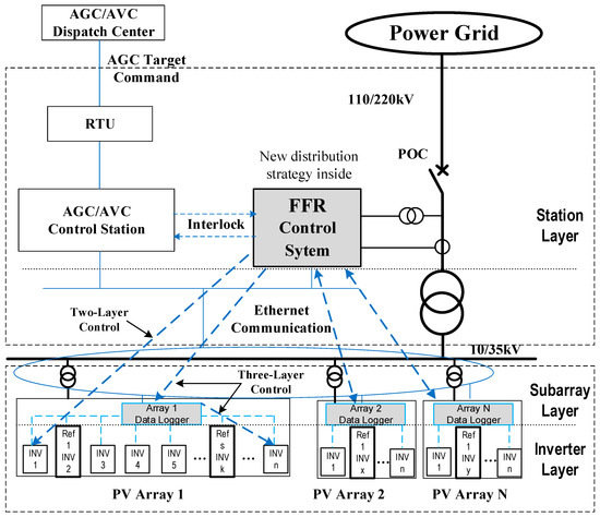
Figure 1.
Two- or three-layer fast frequency response (FFR) control system structure in photovoltaic (PV) power station.
2.1. Response Time Constraint of FFR
In China, the existing AGC power control systems of PV power stations currently perform secondary frequency regulation of the power system, and the regulation time requirements are relatively relaxed, generally reaching the minute level [23,24,25,26,27,28,30,31,32,33,34]. In some countries, this secondary frequency regulation function is implemented in the PPC [34,35,36,37,38]. The much longer minute-scale response time involved in secondary frequency regulation provides immunity to differences in the potential capability values of the inverters or subarrays used in the station. The entire station’s target power can then be approached using an average distribution strategy after multiple rounds of fine tuning of each subarray or power generation unit contained in the station [19,39,40]. Most FFR control systems inherited this average distribution strategy [9,10]. However, in faster primary frequency modulation or FFR frequency modulation tasks, where the time required is much shorter (5 s or less for PV stations in China), the multiple fine-tuning approach based on two or more rounds of tuning is not feasible for most current PV power stations with traditional inverters and communication structures because of time limitations; a single-round precise power response is thus applicable to these power stations [9,10,39,40]. Therefore, a more accurate distribution strategy is required to produce a better response time performance.
2.2. Traditional Average Distribution Strategy
In FFR control systems, apart from the intrinsic system communication structure and the inverter’s power response capability, the first-round power distribution, communication and execution effects are most important [9,41,42,43]. In some conventional PV power stations, several subarrays are selected from among all the subarrays and are set as reference subarrays to evaluate the total PMPC value for the entire power station (as usually required by the PV station’s power prediction system). This means that all the inverters in every selected reference subarray operate in the natural maximum power point tracking (MPPT) mode without a power limit [7,8,32,35,44]. The PMPC value of each subarray is then processed based on the average real power output value of the reference subarrays, and the average strategy is also realized as a result without reflecting the diverse capabilities of the other normal subarrays with different terrains or sun radiance values.
In the AGC systems or FFR control systems in traditional PV power stations, the station control system normally decomposes the total station target power value and then distributes it to all subarrays or inverters by scaling it with respect to their rated capacity(average).
where is the final target power of subarray k (k = 1, 2,…N) and is the total target power value of the station, calculated using the FFR control system or some other station control system.
and are the rated power capacities of the kth and jth subarrays, respectively. is the rated power capacity of the entire station, i.e., the rated capacity of a 10 MW to 100 MW PV power station. These capacities are generally fixed after the commissioning test of the power station. In many PV power stations, the rated capacities of every PV subarray have the same value, and Equation (1) can then be simplified as Equation (2):
This is equivalent to the average power distribution in all subarrays. Therefore, this distribution strategy is also called an average strategy.
In a PV power station with reference subarrays, the reference subarray value is used to help the power station to evaluate the PMPC value for the entire station. The power evaluation strategy for the entire station applies an average of n reference subarrays to all N subarrays of the complete station. The total power evaluation strategy for the entire power station involves the assumption that the station contains N subarrays, among which n subarrays are set as the reference subarrays. The PMPC value of the reference ith subarray is defined as , (i = 1… n), and the average PMPC value of the n reference subarrays in the station is given by in Equation (3):
The average PMPC value of each subarray is defined approximately as , which is equal to the average of these reference subarrays, as given by Equation (4).
The real-time PMPC value for the entire station is then given by:
Generally, all the calculations above are completed in the distribution software module in the station control system, with little participation from the subarray or the inverter. The potential power differences among the scattered PV subarrays are ignored, and it is then easy to develop and deploy this approach for several data acquisitions or setting requirements. This is the most important advantage of this average strategy [20,23,32].
For a PV power station with reference subarrays, the total target power of the station comprises two parts: the power output of the reference subarrays, and the power output of the normal subarrays. However, the reference subarrays do not need to be distributed, and operate in their natural MPPT mode. Then, the remaining target power is equal to the total target power value, minus the accumulated sum of the powers of these reference subarrays (as given in Equation (1)), and this power will be decomposed and allocated among most of the other normal subarrays. The updated distribution equation is given as follows:
2.3. Distribution Effect Analysis of Traditional Average Strategy
In small PV power stations, or in stations with plain areas in cloudless weather, the average power distribution assignment given above is effective because all inverters and PV panels in the subarrays generally have identical or similar power generation capabilities. However, in large-scale PV power stations, e.g., 100 MW-level PV power stations in mountainous areas or in plain areas with clouds, the differences between the PV subarrays become obvious under diverse environmental or sun radiation conditions, and the use of an inappropriate control strategy leads to a deviation from the control target. For example, on the point-of-connection (POC) side after the first round of FFR power distribution, there may be a non-negligible and obvious deviation from the intended target station power value, although the real-time total maximum power generation capability of the power station can still meet the regulation requirements.
To explain how power generation capability differences between the subarrays lead to a poor FFR function implementation effect, a simplified explanation is provided as follows (as shown in Figure 2). Assuming that the total rated power of a PV power station is 100 MW, the station can then be divided into two parts, with 50 MW of power for part A and 50 MW of power for part B. It should be assumed that, at a certain time, the PMPC value of part A is evaluated to be 44 MW for sunny weather because it has better solar radiance and a better geographical environment, while that of part B is evaluated to have a lower value of 38 MW because of cloudy weather and poorer environmental conditions. Therefore, the real-time total power capability value for the entire station is 82 MW. At this time, it is assumed that the target power value calculated using the FFR, based on the demand for frequency regulation, is 80 MW. Because the station’s FFR control system does not know the available PMPC values of either part A or part B, it normally decomposes the 80 MW total evenly into two parts based on equally rated capacities of 40 MW each. For part A, the target 40 MW value will be achieved successfully, with 4 MW of PV power being either curtailed or abandoned. However, for part B, the total power of 38 MW will be the actual power output, because only 38 MW of power is available inside part B. The total power output of the entire station is then only 78 MW, which is 2 MW lower than the original 80 MW target.
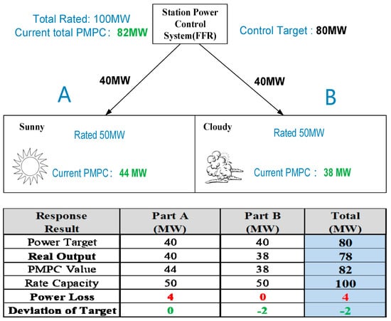
Figure 2.
Power distribution effect of traditional average strategy.
The reason why the unsuccessful power distribution and execution result was obtained for the entire station, as described above, is that unreasonably high distribution values were allocated to subarrays with low PMPC values, while low target values were allocated to subarrays with high PMPC values, thus resulting in their power outputs being capped with subsequent power losses. Finally, this approach leads to power deviation from the FFR target value, with evident power losses and even penalties. Better distribution strategies are expected to aid in improving this performance.
3. Proportional Distribution Strategy Based on Subarray PMPC Value
3.1. Methods to Evaluate the PMPC Value
The problem with the traditional distribution strategy is that it treats each of the subarrays indiscriminately [8,9,23,24]. The solution to this problem is to evaluate the different PMPC values of the inverters and the subarrays efficiently. However, in current PV power stations, no direct data are recorded for the PMPC values of the inverters or subarrays, even in the current PV power station prediction systems [34]. It is a major challenge for a PV power station that maintains reserves to monitor its PMCP value and thus the power headroom available, which varies with irradiance and temperature variations [35].
In [35], a photovoltaic model-based method was proposed, and it summarized that three main different estimation philosophies have been proposed in the literature. These estimation philosophies are: (1) based on irradiance and temperature sensors, (2) based on photovoltaic models, and (3) based on reference inverters. However, the sensor-based method suffers in accuracy because of the inevitable measurement errors and the deviations of the actual PV system parameters [35]. The photovoltaic model-based method is promising and may be beneficial for the implementation of a proportional distribution strategy. At present, however, this method also suffers from two main difficulties in engineering practice: (1) it is difficult to digitalize all types of photovoltaic panel model on the inverter or subarray side; and (2) it is difficult to update the photovoltaic models continuously during long-term operations, particularly when all types of external factors, including dust coverage and panel cracking, are considered. For the remaining reference inverter-based method, the main idea of use of this reference inverter in a traditional control system is that the capabilities of each inverter or subarray are equal in different subarrays at any time. Unlike the traditional scheme, this paper proposes the use of a more accurate estimation scheme, based on reference inverters, to estimate the PMCP of the power station, and specifically the PMCP value for each subarray, which is much more accurate when compared with the traditional equal methods with reference inverters.
The new proposed method for reference inverters involves the scattering of a small number of inverters within each subarray, rather than the gathering of large numbers of reference inverters to form one or several reference subarrays, which means that all inverters in these subarrays work in the MPPT mode with no power limit. The reference inverter in each subarray outputs the actual natural power directly, thus truly reflecting the effects of numerous factors on this subarray, including the sun radiation intensity, the air pressure, temperature, humidity, the panel’s cleanliness, panel tilt, the panel aging level, the photoelectric conversion efficiency, and the line loss. By calculating average values for each inverter based on these scattered reference inverters, the PMPC value can be derived for each subarray. The new distribution strategy proposed later in the paper is based on this approach.
3.2. Proportional Distribution Algorithm
For simplicity, to calculate the PMPC value for a local area or a subarray, we select a PV power station with string inverters as an example. Assuming that there are N subarrays in this power station, and that each subarray contains n inverters, including s reference inverters, there are then n−s units in the subarray involved in power regulation. We detect the respective natural maximum power values for each of the s reference inverters Psi at a specific time t. Then, the average natural maximum power of the s reference inverters in the subarray is , as shown in Equation (7).
The average PMPC value of the inverters within this subarray is then given approximately by Equation (8).
Furthermore, the real-time total PMPC value of this kth subarray is:
It is recommended that the software calculations described above, including that for , are performed in the data logger of each subarray (as shown in Figure 1) according to the principle of nearby distributed deployment. Naturally, the calculations can also be performed in the station-level control system. In this case, the data collection and calculation loads of the station-level acquisition and control system will be comparatively heavy. The real-time PMPC value of the complete station is then given by:
When compared with the PMPC obtained from Equation (5) for the traditional reference subarray-based average strategy, the new strategy proposed above is much more elaborate and accurate. The value determined for the entire power station using the new strategy is accumulated using detailed power capability evaluations of every subarray and power generation component. This is more accurate than using the average value for the reference subarrays, multiplied by the total number of subarrays.
The cost of this approach involves the costs of first setting reference inverters in each subarray, then having the data logger in each subarray collect real-time data from these reference inverters, and subsequently calculating, evaluating, and sending the PMPC value for each subarray to the station control system (e.g., the FFR control system, the AGC, or the PPC). These additional setup, development, and deployment operations and costs represent the shortcomings or difficulties of the newly proposed strategy.
The station-level power control system can then decompose and distribute the station’s total target power, , into each subarray with reference to the real-time PMPC value for each subarray, as given by Equation (11).
where is the final target power of the kth subarray (k = 1, 2,…N). and are the real-time subarray PMPC values of the kth and jth subarrays obtained from Equation (9).
3.3. Distribution Effect Analysis of the Proportional Strategy
Through comparison with Figure 2, the power distribution effect shown in Figure 3 explains the improved effect of the proposed distribution strategy. As long as the total target value remains lower than the total PMPC value of the entire power station, then according to the evaluated PMPC values for the different subarrays or regions, appropriate power target values are allocated that normally lie within the power capability scope of each target subarray. This reduces the total power deviation as far as possible.
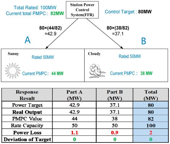
Figure 3.
Power distribution effect of real-time proportional algorithm.
4. Comparison and Analysis of the Two Distribution Strategies
Equation (12) compares the two power distribution strategies. It is not difficult to see that the core idea of both distribution algorithms is to distribute the target values proportionally based on a specific amount. The difference between these methods is that the former strategy corresponds to the constant rated capacity values for the subarrays or inverters, while the latter strategy corresponds to the varying PMPC values for the subarrays.
where is the final target power of the kth subarray (k = 1, 2,…N), and and are the real-time subarray PMPC values for the kth and jth subarrays, respectively, as obtained using Equation (9).
Based on Equations (7)–(9), the real-time PMPC value of the subarray (where k represents the kth subarray in the station) can be obtained based on the reference inverters within each subarray.
4.1. Relationship between the Two Strategies
Under the condition that all inverters in the entire station have the same power generation capability, because they are operating under similar weather and other related conditions, at a specific time T, the PMPC value of each subarray is proportional to its rated capacity, and they share the same percentage value, which is assumed to be c%.
where 0 ≤ c% ≤ 1; then, the key Equation (11) of the proportional strategy can be deduced further, as shown by Equation (14):
In this case, the proportional algorithm evolves into the average algorithm, as given by Equation (1). Furthermore, the rated capacity of each subarray is the same in many PV power stations. Therefore, in these more specific cases, the distribution algorithm given in Equation (14) can be further simplified into the form of Equation (15), which is the same as the equal average distribution strategy given by Equation (2).
The proportional strategy, based on the PMPC values of the subarrays and the reference inverters, contains the traditional average distribution strategy on a higher level. It is thus compatible with the traditional method in certain specific application scenarios.
4.2. Error Performance Comparison between the Two Strategies
Figure 4 shows a comparative error analysis of the two distribution strategies, undertaken to enable a comparison of their error performances. Assuming that there are N subarrays in the station, and by taking the subarrays to be the local areas for the analysis, the maximum, minimum, and average powers generated by each subarray in the station at a specified time are called Pi-max, Pi-min, and Pi-avg, respectively.
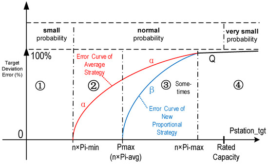
Figure 4.
Deviation error curves of the average and proportional distribution strategies and the probability of error occurrence.
- When Pstation_tgt satisfies the relation Pstation_tgt ≤ N × Pi_min,
The effects of the two distribution strategies are almost identical. The theoretical value of the response error deviation α% (from the deviation rate curve for the average strategy) for the full-station averaging method and the deviation β% (from the deviation rate curve for the proportional distribution) for the proportional distribution strategy are both zero, as shown in zone ① in Figure 4.
- 2.
- When Pstation_tgt increases and satisfies the relationwhere the real-time PMPC value of the entire station is Pmax= N × Pavg, which corresponds to zone ② in Figure 4, the deviation of the average strategy in this area starts to increase, while the deviation of the proportional distribution remains at zero. The two deviation rates in this case are given separately as:N × Pi min ≤ Pstation_tgt ≤ Pmax,
Here, is the actual output of subarray i, and k is the number of subarrays with a PMPC value less than , which is the average power requirement for all the subarrays.
- 3.
- When Pstation_tgt satisfies the relation Pstation_tgt > Pmax,
Pmax is the real-time PMPC value for the entire station, and the proportional strategy deviation β% starts to increase gradually from zero, as shown in Equation (18).
where is the power target value assigned to the ith subarray using the proportional strategy in accordance with the PMPC evaluation results that were obtained based on the reference inverter in each subarray, and Pi is the real-time power output of the ith subarray. The deviation of the average strategy is extended to all subarrays beyond this point (see Equation (19)).
During this period, the deviation of the average strategy is composed of two aspects: first, the PMPC value of the subarray does not reach the required average target value Pstation/N for each subarray, and second, the PMPC value exceeds the Pstation/N value and is limited by the average value of Pstation/N. In contrast, the deviation of the proportional strategy is composed only of the part of the deviation that exceeds the PMPC value of the entire station. In this case, the deviation of the average strategy is obviously greater than that of the proportional strategy.
- 4.
- When Pstation_tgt satisfies the relation Pstation_tgt ≥ N × Pi-max,
The target power value then increases further to reach or even exceed N × Pi-max, and the power value allocated to each subarray via the average strategy must be Pi-max, or may even exceed that value, i.e., the PMPC value of all the subarrays is guaranteed, no more subarrays are operating in the limited power state, and the deviation between the two distribution strategies converges to the following:
The deviations that occur under the two distribution strategies thus reach the same value (i.e., point Q in Figure 4), and the deviation values of the two strategies then remain equivalent thereafter and will gradually approach the limit value of 100% simultaneously.
Figure 4 depicts the complete deviation process for the two strategies. In practice, given that the issued or generated station power target values are mostly lower than the PMPC value for the entire station, i.e., Pstation_tgt < Pmax, corresponding to zones ① and ② in Figure 4, the deviation of the proportional strategy is smaller than that of the average strategy, which means that the regulation response precision of the proportional algorithm is better. The occurrence probability characteristic in Figure 4 shows the occurrence probabilities for the four zones, which were derived from the incomplete probability statistics of some PV power stations.
5. Application Test and Analysis
Recently, the related implementation technologies were tested and verified in onsite FFR application in the Zhengyuan PV power station (which has plain areas with a few small hillsides) in the Inner Mongolia Autonomous Region, China.
The four curves shown in Figure 5 are:
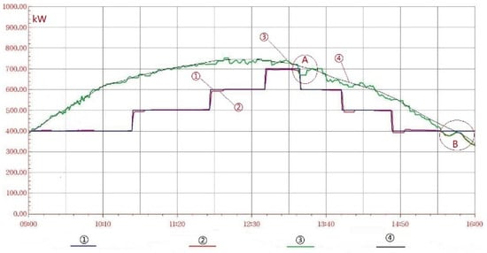
Figure 5.
Power curves for the potential maximum power capability (PMPC) and the real power output in a PV subarray.
- ①
- Subarray target power issued by the station system (blue)
- ②
- Subarray real power output value (red)
- ③
- Subarray real-time PMPC curve (green)
- ④
- Subarray three-day average PMPC curve (black)
5.1. Calculation of Subarray PMPC Value
The Zhengyuan PV power stations are based on string PV subarrays, each of which contains 30 string inverters with a rated power of 33 kW. To test and verify the feasibility of subarray PMPC value calculations based on the reference inverters, a subarray in the Zhengyuan PV power station was selected at random, and the original curves recorded and drawn by the station’s AGC system are shown in Figure 5. The blue curve marked as ① is the target power value given to the target subarray, which was simulated and issued by the station AGC system. The red curve marked as ② is the actual output power value from the target subarray, which was measured using the step-up transformer measurement and control device of the subarray. The green curve marked as ③ is the real-time PMPC value, calculated over one day using the data logger of this subarray based on the reference inverters and using Equations (7)–(9). Finally, the black curve marked as ④ is the three-day average (measured at the same time every day) PMPC value of the subarray.
As shown in circles A and B in Figure 5, when the station’s dispatching target power value exceeds the PMPC value of the subarray, the actual power output curve ② of the subarray is then enveloped or limited by the PMPC value curve ③. This effectively proves that the calculated subarray PMPC value, based on the reference inverters, reflects the actual maximum power output capability of the subarray at that time accurately.
Additionally, the green real-time PMPC value curve ③ is centered around the smoother three-day average PMPC value curve ④. When the target power value of the subarray is lower than the current real-time PMPC value of the subarray, the data logger in the subarray can then control the inverters in the subarray to limit the power output to the target value (limited power mode).
In addition, five representative subarrays (in the flat area, at the top of a hillside, on a bright hillside, on a shady hillside, and at the bottom of a hillside) in the Zhengyuan PV power station were selected as five typical generation components for research. One inverter was selected from every 30 inverters in each of the five subarrays to act as a reference inverter (the test conditions and workloads limited the selection of additional reference inverters in each subarray, although that would be preferable). The site record started at a time T (e.g., 10 am, 2 pm) on a specified day in October, as shown in Table 1. Then, Equation (9) was used to calculate the PMPC value tables for each subarray, starting at time T.

Table 1.
Comparison of calculated potential power with real output power.
During the test period, all inverters in these five subarrays were in the natural maximum power (i.e., not limited) state; the true natural power output values of the five subarrays were then recorded every 5 s using the station’s supervisory control and data acquisition (SCADA) system. The values at six representative specific time instants, designated T0, T0 + 5 s, T0 + 5 min, T0 + 15 min, T0 + 30 min, and T0 + 1 h, were recorded as shown in Table 1.
According to Table 1, the maximum absolute error between the PMPC values, calculated based on the reference inverters and the real natural maximum power output values, obtained using all the inverters in these subarrays is 1.68%, and the average absolute error is 0.93%.
A comparative analysis of the curves and data presented above shows that the absolute error between the subarray PMPC value, calculated based on the reference inverter and the actual measured maximum power output value of the subarray, is <2%.
5.2. Response Performance Comparison of FFR Based on Different Strategies
In this power station, ten subarrays were selected to form a virtual 10 MW power station for two different strategies based on the FFR control response test. The test data is shown in Table 2. The testing recorded different distribution strategies for different power capability and frequency disturbance types.
Table 2.
Test Record of Different Distribution Strategies.
The test results in Table 2 show that, when the frequency is disturbed upward and the PV power station needs to either reduce or suppress its output power, the difference between the two strategies is very small. Both strategies can normally meet the system requirements in this case (nos. 1–6 are based on the average strategy and nos. 7–12 are based on the proportional strategy).
The difference between the two strategies is mainly illustrated during a downward frequency disturbance, namely, when the PV power station is required to increase its output power. This is particularly important in the case where the target power is close to the theoretical PMPC value of the entire power station. In this case, it is sometimes difficult to reach the target power point for the entire station when using the average strategy (see nos. 15, 16, 19, 20), although the target value at that time was lower than the station’s theoretical PMPC value. This resulted in an FFR response failure to generate the target power (for a clear comparison, several rounds of fine tuning were not used in the average strategy; if they had been used, the response time would still not have been satisfied). In contrast, the proportional distribution strategy can reach the target power point successfully in almost all cases, which even occurs in some cases where the target power is very close to the power station’s theoretical PMPC (see nos. 21–28). This strategy is thus suitable for use in fast frequency modulation applications in a variety of situations and offers a broader range of application scenarios.
5.3. Analysis of Typical FFR Response Based on the Two Strategies
Figure 6 shows the FFR response curve obtained when using the average strategy during an upward disturbance of the power grid frequency (related to no. 3 in Table 2). This curve indicates that the system can provide the adaptive fast frequency modulation power regulation response for the entire station, with the required response time and accuracy. A small overshoot will sometimes occur, but the system soon returns to the target value.
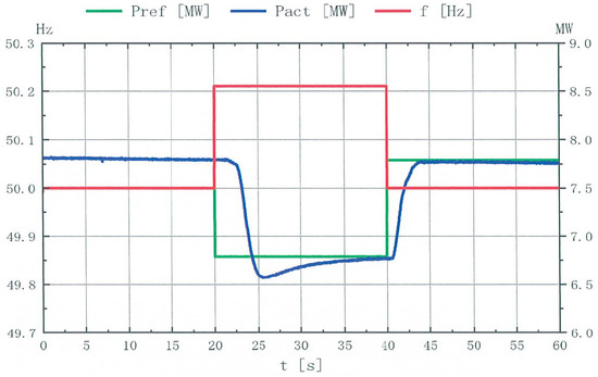
Figure 6.
Frequency upward step with successful FFR (average) response waveform.
Figure 7 shows the FFR response curve obtained when using the proportional distribution strategy during an upward disturbance. This type of upward frequency disturbance requires the power station to reduce its power. The effects of these two strategies are similar and they can both probably meet the power grid’s requirements.
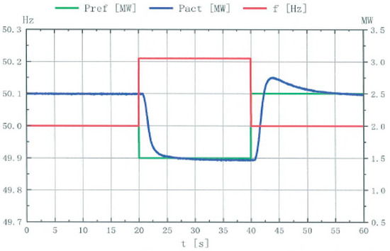
Figure 7.
Frequency upward step with successful FFR (proportional) response waveform.
However, when a downward frequency disturbance requires the power station to increase its output power, and particularly when the frequency modulation target power is close to the evaluated PMPC value of the power station, the frequency modulation response results obtained for the two strategies differ significantly. Figure 8 shows an unsuccessful FFR, obtained with the average strategy response curve for a power grid downward frequency disturbance (related to no. 19 in Table 2). At that time, the evaluated PMPC value of the station was approximately 7.05 MW. When the system frequency made a downward step to 49.79 Hz, the regulation target value of the FFR was required to increase by 1 MW from the original value of 5.95 MW to 6.95 MW. However, after the demand was distributed evenly to each subarray, the total output power from the entire station was only 6.67 MW, which represents a deviation of 0.28 MW. When compared with the target power increment demand of 1 MW, the response error reached 28% (the system error for the entire station’s 10 MW output was 2.8%).
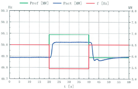
Figure 8.
Frequency downward step with unsuccessful FFR (average) response waveform.
Figure 9 shows the successful FFR obtained in a similar scenario when using the proportional strategy for a power grid downward frequency disturbance (related to no. 25 in Table 2). At that time, the evaluated PMPC value of the station was approximately 7.10 MW. The regulation target value of the FFR during the downward disturbance was to increase by 1 MW from the original value of 5.99 MW to 6.99 MW. The proportional distribution strategy successfully achieved an output of 6.95 MW, with only a 2% deviation error (0.2% for the overall system error).
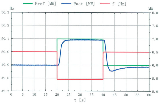
Figure 9.
Frequency downward step with successful FFR (proportional) response waveform.
6. Conclusions
With the increasing proportion of RES energy usage in power systems, these new energy sources are now urgently required to provide high FFR performance to ensure reliable and safe operation of their power systems [1,6,45]. Among the attempts to address the problems of power deviation, losses, and response timeouts in current PV power station FFR processes, this paper analyzes the power distribution strategies for station control systems systematically. Particular emphasis is placed on FFR, and a new power distribution strategy is proposed based on the PMPC value of each subarray, which can be evaluated using internal reference inverters. It is proved in FFR application tests that the proportional distribution strategy, based on the different PMPC values of each subarray, provides better performance with reduced power deviation and faster response speeds. This is particularly important when the system requires the power station to increase its output power. It is also confirmed that the proposed proportional strategy contains the traditional average distribution strategy at a higher level. The proposed strategy is compatible with the traditional method in certain specific application scenarios. Finally, a comparative analysis of the response deviations that occurred during use of the different strategies has also been presented.
Based on the analysis and tests described above, it is possible to predict that the proportional distribution strategy may provide better performances in other station-level control applications in the future, e.g., active or reactive power control from a dispatching center. However, such applications will be considered in future studies.
Author Contributions
Writing—original draft, Software, Visualization, Supervision, S.W.; Resources, Formal analysis, S.D.; Data curation, Investigation, S.D. and G.M.; Writing—review and editing, Resources, G.M.; Methodology, Project administration, Y.L. All authors have read and agreed to the published version of the manuscript.
Funding
This research received no external funding.
Data Availability Statement
Not applicable.
Acknowledgments
The authors appreciate the Inner Mongolia Zhengyuan photovoltaic power station for supporting site testing as well as the provision of working face data.
Conflicts of Interest
The authors declare no conflict of interest.
Abbreviations
| FFR | fast frequency response |
| RES | renewable energy source |
| PV | photovoltaic |
| PMPC | potential maximum power capability |
| AGC | automatic generation control |
| AVC | automatic voltage control |
| PPC | power plant controller |
| POC | point of connection |
| MPPT | maximum power point tracking |
| SCADA | supervisory control and data acquisition |
References
- Zhang, J.; Li, M. Analysis of the Frequency Characteristic of the Power Systems Highly Penetrated by RES Generation. Proc. CSEE 2020, 40, 119–128. [Google Scholar]
- Ferro, G.; Robba, M.; Sacile, R. A Model Predictive Control Strategy for Distribution Grids: Voltage and Frequency Regulation for Islanded Mode Operation. Energies 2020, 13, 2637. [Google Scholar] [CrossRef]
- U.S. Department of Energy. 20% Wind Energy by 2030: Increasing Wind Energy’s Contribution to US Electricity Supply. 2008. Available online: https://www.energy.gov/sites/prod/files/2013/12/f5/41869.pdf (accessed on 25 September 2021).
- Chang, J.; Du, Y.; Lim, E.G.; Wen, H.; Li, X. Coordinated frequency regulation using solar forecasting based virtual inertia control for islanded microgrids. IEEE Trans. Sustain. Energy 2021, 12, 2393–2403. [Google Scholar] [CrossRef]
- Morren, J.; de Haan, S.W.H.; Kling, W.L. Wind turbines emulating inertia and supporting primary frequency control. IEEE Trans. Power Syst. 2006, 21, 433–434. [Google Scholar] [CrossRef]
- Peng, Y.; Liu, T.; Blaabjerg, F. Coordination of virtual inertia control and frequency damping in photovoltaic systems for optimal frequency support. CPSS Trans. Power Electron. Appl. 2020, 5, 305–316. [Google Scholar] [CrossRef]
- Nguyen, N.; Pandit, D.; Quigley, R.; Mitra, J. Frequency response in the presence of renewable generation: Challenges and opportunities. IEEE Open Access J. Power Energy 2021, 8, 543–556. [Google Scholar] [CrossRef]
- Hua, G.; Hu, R.; Jiao, L. Research and application of fast frequency response technology for photovoltaic stations. Power Syst. Clean Energy 2019, 35, 21–26. [Google Scholar]
- Ma, X.; Xu, H.; Liu, X. A test method for fast frequency response function of renewable energy stations in northwest power grid. Power Syst. Technol. 2020, 44, 31–36. [Google Scholar]
- Chu, Y. Actual measurement and analysis of fast response capability value of photovoltaic plants participating in the frequency regulation of northwest power grid. In Proceedings of the 2019 IEEE 8th International Conference on Advanced Power System Automation and Protection (APAP), Xi’an, China, 21–24 October 2019; pp. 825–829. [Google Scholar]
- Fang, Y.; Zhao, S.; Du, E.; Li, S.; Li, Z. Coordinated operation of concentrating solar power plant and wind farm for frequency regulation. J. Mod. Power Syst. Clean Energy 2021, 9, 751–759. [Google Scholar] [CrossRef]
- Conte, F.; Schiapparelli, G.P. Day-ahead and intra-day planning of integrated BESS-photovoltaic systems providing frequency regulation. IEEE Trans. Sustain. Energy 2020, 11, 1797–1806. [Google Scholar] [CrossRef]
- Zhang, W.; Sheng, W.; Duan, Q. Automatic generation control with virtual synchronous renewables. J. Mod. Power Syst. Clean Energy 2022, 2, 1–13. [Google Scholar]
- Xin, H.; Liu, Y.; Wang, Z. A frequency regulation strategy for photovoltaic systems wind energy storage. IEEE Trans. Sustain. Energy 2013, 4, 985–993. [Google Scholar] [CrossRef]
- Liu, Y.; Ying, K.; Xin, H. A control strategy for photovoltaic generation system based on quadratic interpolation method. Autom. Electr. Power Syst. 2012, 36, 29–35. [Google Scholar]
- Zhong, C.; Zhou, S.; Yan, G. A new frequency regulation control strategy for photovoltaic power plant based on variable power reserve level control. Trans. China Electrotech. Soc. 2019, 34, 1013–1024. [Google Scholar]
- Jin, G.; Luo, A.; Chen, Y. Proportional load sharing for parallel inverter systems based on modified P-V droop coefficient. Trans. China Electrotech. Soc. 2016, 31, 34–38. [Google Scholar]
- Jiang, W.; Gao, Y.; Ding, X. Power allocation method for improving efficiency of grid-connected inverters under parallel operation. Autom. Electr. Power Syst. 2017, 41, 46–53. [Google Scholar]
- Wang, S.; Duan, S.; Hou, W. Research and application on a hierarchical distributed control structure based AGC technology for photovoltaic power stations. Autom. Electr. Power Syst. 2016, 40, 126–132. [Google Scholar]
- Ma, L.; Li, Y.; Chang, X. An active power distribution strategy for photovoltaic power station with multi-inverter. Power Technol. 2018, 42, 1379–1382. [Google Scholar]
- Chiandone, M.; Campaner, R.; Bosich, D.; Sulligoi, G. A Coordinated voltage and reactive power control architecture for large PV power plants. Energies 2020, 13, 2441. [Google Scholar] [CrossRef]
- Zhu, H.; Shen, W.; Dong, K. Research on active power control strategy of large photovoltaic power plant. Electr. Technol. 2019, 4, 82–85. [Google Scholar]
- Dong, Y.; Ren, N.; Wang, J. Automatic control method of active power in photovoltaic power station and its implementation. Electr. Technol. 2019, 7, 18–24. [Google Scholar]
- Wang, Y. Research on active power control technology of photovoltaic power station. Eng. Technol. Appl. 2019, 7, 34–39. [Google Scholar]
- Anand, S.; Dev, A.; Sarkar, M.K.; Banerjee, S. Non-fragile approach for frequency regulation in power system with event-triggered control and communication delays. IEEE Trans. Ind. Appl. 2021, 57, 2187–2201. [Google Scholar] [CrossRef]
- Ehtesham, M.; Rana, S.A.; Ali, S.; Jamil, M. Inverter control strategy for enabling voltage and frequency regulation of grid connected photovoltaic system. In Proceedings of 2018 IEEE 8th Power India International Conference (PIICON), Haryana, India, 10–12 December 2018; pp. 1076–1082. [Google Scholar]
- Varma, R.K. Simultaneous fast frequency control and power oscillation damping by utilizing photovoltaic solar system as photovoltaic-STATCOM. IEEE Trans. Sustain. Energy 2020, 11, 415–425. [Google Scholar] [CrossRef]
- Varma, R.K.; Salehi, R. SSR mitigation with a new control of photovoltaic solar farm as STATCOM (photovoltaic-STATCOM). IEEE Trans. Sustain. Energy 2017, 8, 1473–1483. [Google Scholar] [CrossRef]
- Yan, G.; Hu, W.; Jia, Q. Single-stage grid-connected photovoltaic generation takes part in grid frequency regulation for electromechanical transient analysis. In Proceedings of the 2019 IEEE PES Innovative Smart Grid Technologies Asia, Chengdu, China, 21–24 May 2019; pp. 536–547. [Google Scholar]
- Hu, B.; Lou, S.; Li, H. Spinning reserve demand estimation in power systems integrated with large-scale photovoltaic power stations. Autom. Electr. Power Syst. 2015, 39, 15–19. [Google Scholar]
- Wang, S.; Sun, G.; Yu, C. Photovoltaic power generation system level rapid power control technology and its application. Proc. CSEE 2018, 38, 6254–6263. [Google Scholar]
- Sun, X.; Liu, X.; Cheng, S. Actual measurement and analysis of FFR capability value of photovoltaic-inverters in northwest power grid. Power Syst. Technol. 2017, 41, 25–31. [Google Scholar]
- Jia, Q.; Yan, G.; Zhang, S. Dynamic coordination mechanism of grid frequency regulation with multiple photovoltaic generation units. Autom. Electr. Power Syst. 2019, 43, 59–65. [Google Scholar]
- Ge, L.; Xian, Y.; Yan, J.; Wang, B.; Wang, Z. A hybrid model for short-term PV output forecasting based on PCA-GWO-GRNN. J. Mod. Power Syst. Clean Energy 2020, 8, 1268–1275. [Google Scholar] [CrossRef]
- Batzelis, E.I.; Junyent-Ferre, A.; Pal, B.C. MPP Estimation of PV Systems keeping Power Reserves under Fast Irradiance Changes. In Proceedings of the 2020 IEEE Power & Energy Society General Meeting (PESGM), Brampton, ON, Canada, 2–6 August 2020; pp. 1–5. [Google Scholar] [CrossRef]
- Perez, M.; Perez, R.; Hoff, T.E. Least-cost firm PV power generation: Dynamic curtailment vs. inverter-limited curtailment. In Proceedings of the 2021 IEEE 48th Photovoltaic Specialists Conference (PVSC), Fort Lauderdale, FL, USA, 20–25 June 2021; pp. 1737–1741. [Google Scholar]
- Syafrianto, D.; Marojahan, K.; Nahor, B. Optimized allocation of solar pv in batam-bintan power system 2021–2025. In Proceedings of the 2021 3rd International Conference on High Voltage Engineering and Power Systems (ICHVEPS), Bandung, Indonesia, 5–6 October 2021; pp. 149–154. [Google Scholar]
- Bharatee, P.K.; Ghosh, A. A power management scheme for grid connected PV integrated with hybrid energy storage system. J. Mod. Power Syst. Clean Energy 2021, 10, 954–963. [Google Scholar] [CrossRef]
- Wu, Z.; Jiang, Z.; Yang, X. An improved global MPPT method based on power closed-loop control. Power Syst. Prot. Control 2018, 46, 57–62. [Google Scholar]
- Tang, Y.; Wang, Q.; Chen, N. An optimal active power control method of wind farm based on wind power forecasting information. Proc. CSEE 2012, 32, 1–7. [Google Scholar]
- Jin, W.; Xu, S.; Zhang, D. Application and response time test of mw-level battery energy storage system used in photovoltaic power station. High Volt. Eng. 2017, 43, 2425–2432. [Google Scholar]
- Zhu, X.; Liu, S.; Zhang, H. Sliding mode control based direct voltage/power control strategy photovoltaic Grid-connected inverters under unbalanced grid voltage. Power Syst. Prot. Control 2016, 44, 133–140. [Google Scholar]
- Sun, X.; Cheng, S.; Liu, X. Test method for the frequency characteristics of the northwest power grid. Power Syst. Prot. Control 2018, 42, 148–152. [Google Scholar]
- Kato, T.; Kimpara, Y.; Tamakoshi, Y. An experimental study on dual P-f droop control of photovoltaic power generation for supporting grid frequency regulation. In Proceedings of the 10th Symposium on Control of Power and Energy Systems (CPES2018), Tokyo, Japan, 4–6 September 2018; pp. 130–138. [Google Scholar]
- Hoke, A.F.; Shirazi, M.; Chakraborty, S. Rapid active power control of photovoltaic system for grid frequency support. IEEE J. Emerg. Sel. Top. Power Electron. 2017, 5, 1154–1163. [Google Scholar] [CrossRef]
Publisher’s Note: MDPI stays neutral with regard to jurisdictional claims in published maps and institutional affiliations. |
© 2022 by the authors. Licensee MDPI, Basel, Switzerland. This article is an open access article distributed under the terms and conditions of the Creative Commons Attribution (CC BY) license (https://creativecommons.org/licenses/by/4.0/).