Blind Source Separation of Transformer Acoustic Signal Based on Sparse Component Analysis

Abstract

In the acoustics-based power transformer fault diagnosis, a transformer acoustic signal collected by an acoustic sensor is generally mixed with a large number of interference signals. In order to separate transformer acoustic signals from mixed acoustic signals obtained by a small number of sensors, a blind source separation (BSS) method of transformer acoustic signal based on sparse component analysis (SCA) is proposed in this paper. Firstly, the mixed acoustic signals are transformed from time domain to time–frequency (TF) domain, and single source points (SSPs) in the TF plane are extracted by identifying the phase angle differences of the TF points. Then, the mixing matrix is estimated by clustering SSPs with a density clustering algorithm. Finally, the transformer acoustic signal is separated from the mixed acoustic signals based on the compressed sensing theory. The results of the simulation and experiment show that the proposed method can separate the transformer acoustic signal from the mixed acoustic signals in the case of underdetermination. Compared with the existing denoising methods of the transformer acoustic signal, the denoising results of the proposed method have less error and distortion. It will provide important data support for the acoustics-based power transformer fault diagnosis.

1. Introduction

As an important hub of equipment in the power grid, power transformers play a key role in the safe and stable operation of the power system. During the operation of the transformer, an acoustic signal is generated by the vibration of the transformer core and winding, which contains rich status information about the transformer. Transformer fault diagnosis can be realized by accurately detecting and analyzing the transformer acoustic signal [1,2]. However, due to the presence of various interference signals including power equipment sound, speech sound and vehicle sound at the transformer substation site, the transformer acoustic signal collected by the acoustic sensor may be mixed with a large number of interference signals, which will seriously affect the accuracy of transformer fault diagnosis [3]. Therefore, the accuracy of the acoustics-based transformer fault diagnosis can be improved by accurately extracting the transformer acoustic signal.

In general, noise suppression methods of transformer acoustic signal include wavelet domain denoising [4,5,6], empirical mode decomposition (EMD) denoising [7,8], source separation technology based on clustering algorithm [9,10,11] and BSS [12,13,14], etc. Pan et al. [4] proposed a layered threshold denoising algorithm of acoustic signals, which has higher accuracy in transformer acoustic signal denoising than conventional methods. Wu et al. [6] used wavelet packet transform (WPT) and 50 Hz frequency doubling comb filter to separate transformer acoustic signal from noisy signals. Although the experimental results in [4,6] show that the wavelet denoising method has a good denoising effect, the wavelet basis function and decomposition levels are required to be manually determined, which directly affects the denoising effect of the transformer acoustic signal. Liu et al. [7] proposed signal denoising of high voltage cable partial discharge based on EMD-BSS, it not only effectively removes the noise in the partial discharge signal but also retains the integrity of the PD signal well. However, the phenomenon of model aliasing and boundary effects will be produced when EMD is used to decompose non-stationary signals; it is difficult to completely separate transformer acoustic signals and interference signals by using the EMD denoising method. Source separation technology based on a clustering algorithm is carried out by extracting the specific behavior (temporal or spectral) of each type of pulse source and clustering the feature quantities, it is mainly used for the separation of partial discharge (PD) signal. Hao et al. [9] proposed a discrimination method for multiple PD sources using wavelet decomposition and principal component analysis, which successfully separated multiple PD sources. The method is mainly used for the separation of multiple pulse signals, but the transformer acoustic signal and part of the interference signals are continuous signals, and the specific behavior (temporal or spectral) of the interference signals are similar, which directly affects the separation effect of the transformer acoustic signal. BSS is the process of separating source signals from mixed signals collected by sensors when the sound sources and mixing process are unknown [15]. A BSS algorithm based on independent component analysis has been widely used in the fields of transformer vibration and PD signal denoising [16,17,18], but this method has an underdetermined problem, which must meet the condition that the number of acoustic sensors is more than or equal to the number of source signals. In the acoustics-based transformer fault diagnosis, due to the unknown number of sound sources at the transformer substation site, the limited number of acoustic sensors, and the influence of various environmental interference signals, the separation of transformer acoustic signal is a typical underdetermined BSS problem. In recent years, SCA based on sparse representation theory has gradually become a powerful means to solve the problem of underdetermined BSS. The process of separating source signals using the method includes two stages: estimating the mixing matrix by signals sparsity and clustering algorithm and recovering the source signals by L₁ norm decomposition [19,20,21]. Bofill et al. [19] proposed an underdetermined blind source separation method using sparse representations, which successfully separated six source signals from two mixed acoustic signals. Li et al. [21] used density peak clustering and compression sensing model to separate various fault signals from mixed vibration signals, and the separation effect is good.

Based on the above analysis, we applied sparse component analysis to denoising of transformer acoustic signal and proposed a blind source separation method of transformer acoustic signal based on sparse component analysis. The proposed method is used to denoise the simulated and measured transformer acoustic signals, and the results show that the transformer acoustic signal can be separated from the mixed acoustic signals under the condition of being underdetermined.

2. Principle of Blind Source Separation for Transformer Acoustic Signal

2.1. Characteristic Analysis of Interference Signals

In the acoustics-based power transformer fault diagnosis, the transformer acoustic signal generated by the core and winding vibration is considered a useful signal, and the acoustic signal generated by the external sound source of the transformer is regarded as an interference signal. In addition, the electronic circuit of the sound acquisition system also generates electrical noise. Since the electrical noise can be suppressed by high-quality sound collection equipment, this paper only deals with the interference signals of the transformer acoustic signal.

According to the field investigation and analysis, the external sound sources of transformer substations include transformers, capacitors, reactors and high-voltage transmission lines. The sound of the transformer is mixed by the acoustic signal of the transformer core and winding, the sound of the cooling fan and the action sound of the on-load tap changer (OLTC). Sound signals will also be generated by capacitors, reactors and the corona discharge of high-voltage transmission lines. Besides, there may be various environmental interference signals such as speech sound, vehicle sound and bird sound in the transformer operation environment. All the above sound signals may be interference components of the transformer acoustic signal. This paper classifies and lists the possible interference signals in the transformer operation environment according to the characteristics of interference signals, the results are shown in

Table 1. Classification and main characteristics of interference signals.

Interference Source	Interference Factor	Duration/s	Frequency Band/Hz
Transformer structure	Cooling fan sound	continued	0–1000
	OLTC action sound	0.2	0–20,000
power equipment	Reactor sound	continued	0–2000
	Capacitor sound	continued	0–2000
	Corona discharge sound	continued	5000–20,000
operation environment	Speech sound	0.4	150–5000
	Musical sound	0.5	0–20,000
	vehicle sound	0.5	2000–8000
	Bird sound	0.2	3000–8000

.

From Table 1, it can be seen that the types of interference signals in the transformer acoustic signals are relatively complex. Firstly, the distance between the reactor, capacitor and transformer is far, so the interference signals generated by the capacitor and reactor during operation can be filtered by the single directional acoustic sensor. Therefore, they may not be considered. Other interference signals can be divided into two categories: one is the interference signal, which has no intersection with the frequency band (0–1000 Hz) of the transformer acoustic signal, including corona discharge sound, vehicle sound and bird sound; the other is the interference signal which has a large intersection with the frequency band of transformer acoustic signal, including OLTC action sound, Speech sound and Musical sound.

The first kind of interference signal can be easily eliminated by a low-pass filter. Nevertheless, the frequency band of the second type of interference signal overlaps with that of the transformer acoustic signal, it is necessary to use BSS based on SCA to get rid of the second type of interference signal.

2.2. Sparse Component Analysis

The sparse component analysis method uses the sparsity of signals to solve the underdetermined problem. In the underdetermined condition where the number of source signals is more than that of acoustic sensors, the BSS problem of the mixed acoustic signals in a substation can be described as

$$\mathit{X}(t)=\mathit{\text{AS}}(t)={\sum }_{n=1}^N{\mathit{a}}_n{S}_n(t)$$

(1)

where X(t) = [X₁(t),X₂(t),...,X_M(t)]^T are the M mixed acoustic signals at time t, A ∈ $ℝ$^M×N is the unknown mixing matrix with M < N, a_n = [a_1n,a_2n, ..., a_mn]^T is the nth column of the mixing matrix A. S(t) = [S₁(t),S₂(t),...,S_N(t)]^T are the N sound source signals at time t.

For most of the sampling points, the amplitudes of the sparse signal are zero or close to zero. In other words, it is definite that the amplitude of only one source signal is non-zero at the same sampling point if all sound source signals meet the sparse condition. Hence, most sampling points have only one sound source signal dominant, while the amplitude of other sound source signals is zero, these sampling points are called single source points. For the convenience of explanation, assume that the number of acoustic sensors is 2, i.e., M = 2, and only one sound source signal S₁ is present at a single source point t, i.e., S₁(t) ≠ 0 and S₂(t) = 0. Equation (1) can be simplified as

$${\mathit{X}(t)=\mathit{a}}_1{S}_1(t)$$

(2)

Thus, the amplitude ratio of the two components of the mixed acoustic signals is

$$\alpha =\frac{X_1(t)}{X_2(t)}=\frac{a_{11}{S}_1(t)}{a_{21}{S}_1(t)}=\frac{a_{11}}{a_{21}}$$

(3)

From (3) it can be seen that the SSPs dominated by the sound source signal S₁ will be distributed on a straight line where the direction is a₁. Therefore, the SSPs dominated by different sound source signals will be distributed on straight lines in different directions. The direction of the lines can be calculated by clustering algorithm and used as the estimation of the column vectors of the mixing matrix so that the transformer acoustic signal can be separated [19].

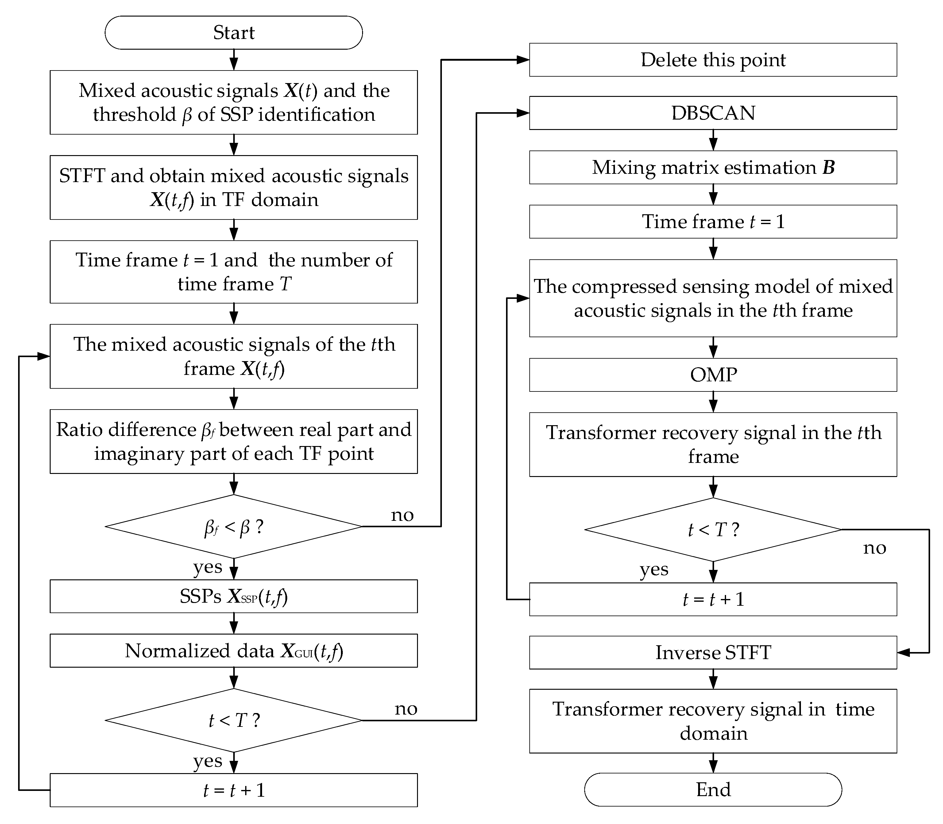
3. Blind Source Separation Method of Transformer Acoustic Signal

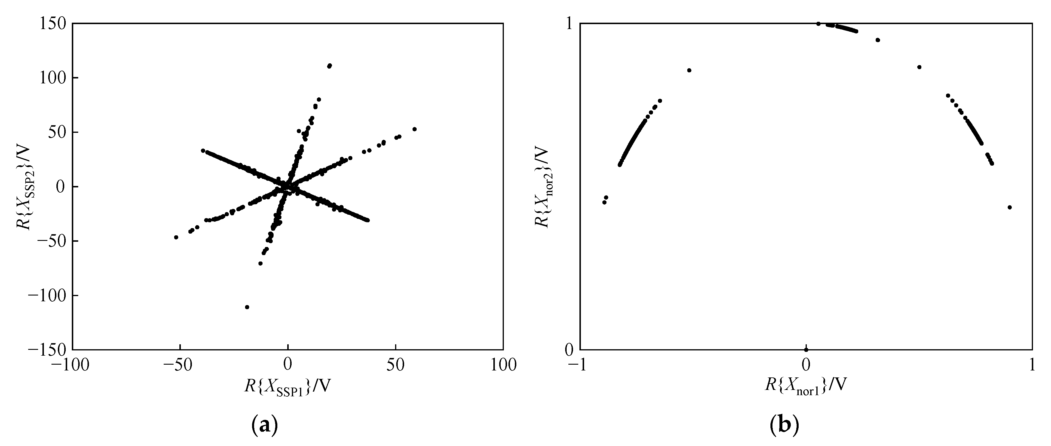
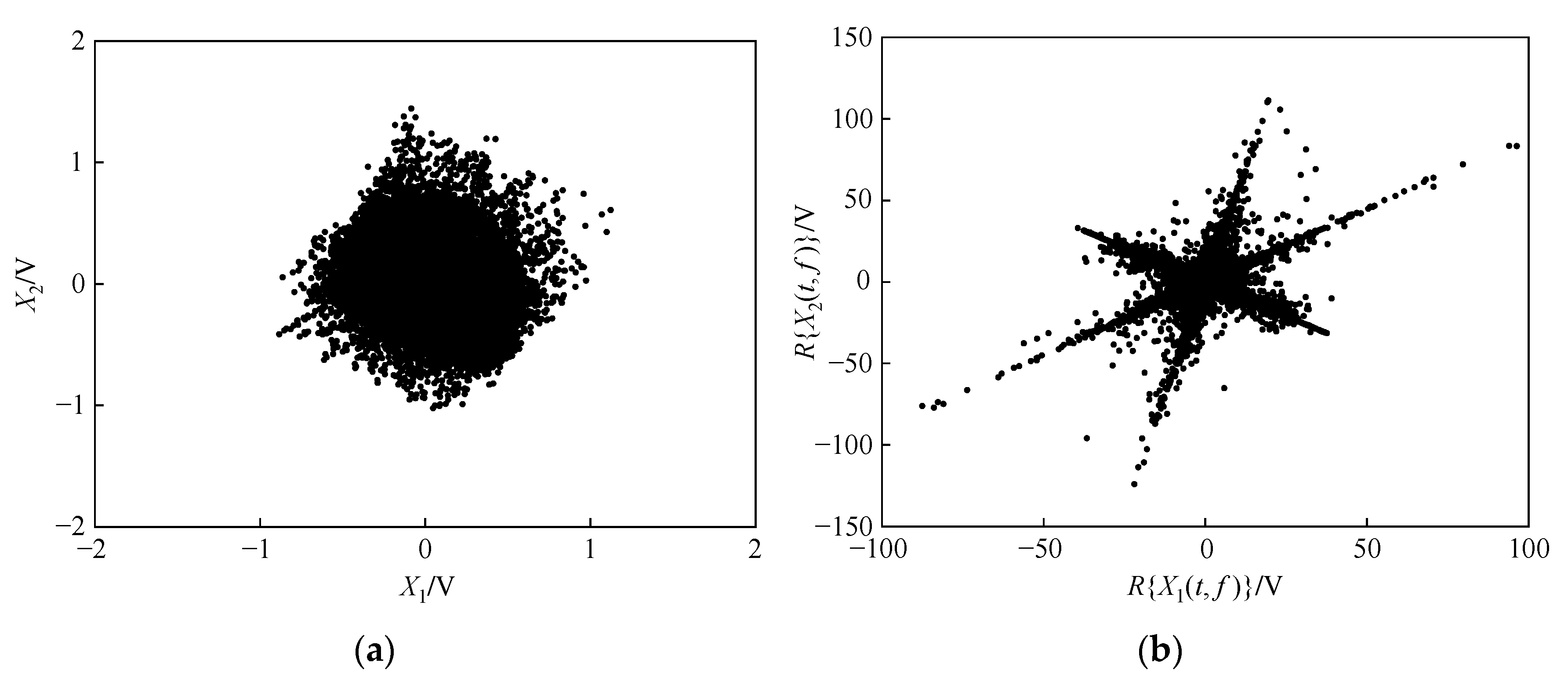
3.1. Sparse Enhancement of Mixed Acoustic Signals

The sparsity of sound source signals is the key factor of SCA. However, the transformer acoustic signal and its interference components cannot meet the sparsity requirements of SCA in practice, the mixed acoustic signals are transformed from the time domain to the TF domain. The underdetermined BSS model in (1) can be expressed domain using short-time Fourier transform (STFT) as

$$\mathit{X}(t,f)=\mathit{\text{AS}}(t,f)={\sum }_{n=1}^N{\mathit{a}}_n{S}_n(t,f)$$

(4)

where X(t, f) = [X₁(t, f), X₂(t, f), ..., X_M(t, f)]^T and S(t, f) = [S₁(t, f), S₂(t, f), ..., S_N(t, f)]^T are, respectively, the STFT coefficients of the mixed acoustic signals and sound source signals in the fth frequency bin at time frame t. Although the mixed acoustic signals show approximate sparsity in the TF plane, it does not meet the sparsity requirements of SCA. Therefore, the SSPs are selected from the mixed acoustic signals in the TF plane by the single-source-point identification method based on phase angle. Assume that only one source signal S₁ is present at an SSP (t₁, f₁) in the TF plane. Equation (4) can be expressed as

$${\mathit{X}(t}_1{,f}_1{)=\mathit{a}}_1{S}_1{(t}_1{,f}_1)$$

(5)

Calculating the real and imaginary parts of each component of the mixed acoustic signals X(t₁, f₁), we will get

$${R\text{{}X}_m{(t}_1{,f}_1{)\text{}}=a}_{m1}{R\text{{}S}_1{(t}_1{,f}_1)\text{}}$$

(6)

$${I\text{{}X}_m{(t}_1{,f}_1{)\text{}}=a}_{m1}{I\text{{}S}_1{(t}_1{,f}_1)\text{}},m=1,2,...,M$$

(7)

where R{X} and I{X} are the real and imaginary parts of X, respectively. The angle between R{X_m(t₁, f₁)} and I{X_m(t₁, f₁)} can be expressed as

$${\mathsf{\theta }=\tan }^{-1}\left(\frac{{R\text{{}X}_1{(t}_1{,f}_1)\text{}}}{{I\text{{}X}_1{(t}_1{,f}_1)\text{}}}\right){=\text{…}=\tan }^{-1}\left(\frac{{R\text{{}X}_M{(t}_1{,f}_1)\text{}}}{{I\text{{}X}_M{(t}_1{,f}_1)\text{}}}\right)$$

(8)

From (8) it can be seen that the phase angles of each component of the mixed acoustic signals are the same. That is to say, the ratio of the real part to the imaginary part of each component of X(t, f) will be the same if the sampling point (t, f) is an SSP. However, the probability of obtaining SSPs is very low in practice, hence we relax the determination condition of SSP as follows: the point in the TF plane where the absolute value of the difference β_f between the ratio of the real part to the imaginary part of each component of the mixed acoustic signals is less than $\beta$ is taken as an SSP. The SSP identification formula can be expressed as

$$\left|\frac{{R\text{{}X}_I{(t}_1{,f}_1)\text{}}}{{I\text{{}X}_I{(t}_1{,f}_1)\text{}}}-\frac{{R\text{{}X}_J{(t}_1{,f}_1)\text{}}}{{I\text{{}X}_J{(t}_1{,f}_1)\text{}}}\right|<\beta ,I\ne J$$

(9)

where $\left|X\right|$ is the absolute value of X; I and J are the subscripts of different components of the mixed acoustic signals respectively.

After single-source-point identification in the TF plane, the SSPs X_SSP show sufficient sparsity and linear clustering characteristics. In order to ensure that the direction of each line is represented by a unique direction vector, the negative direction vectors of X_SSP are mapped to the positive half unit circle using the normalization method. The transformation process can be expressed as

$${\mathit{X}}_{\mathrm{nor}}(t,f)=\left\{\begin{array}{c}\frac{{\mathit{X}}_{\mathrm{SSP}}(t,f)}{‖{\mathit{X}}_{\mathrm{SSP}}(t,f)‖}{,\mathit{X}}_{\mathrm{SSP}}(t,f)>0\\ \frac{{-\mathit{X}}_{\mathrm{SSP}}(t,f)}{‖{\mathit{X}}_{\mathrm{SSP}},(t,f)‖}{,\mathit{X}}_{\mathrm{SSP}}(t,f)<0\end{array}\right.$$

(10)

where ${‖X‖=(X}^T{X)}^{1/2}$ is the absolute value of the vector X.

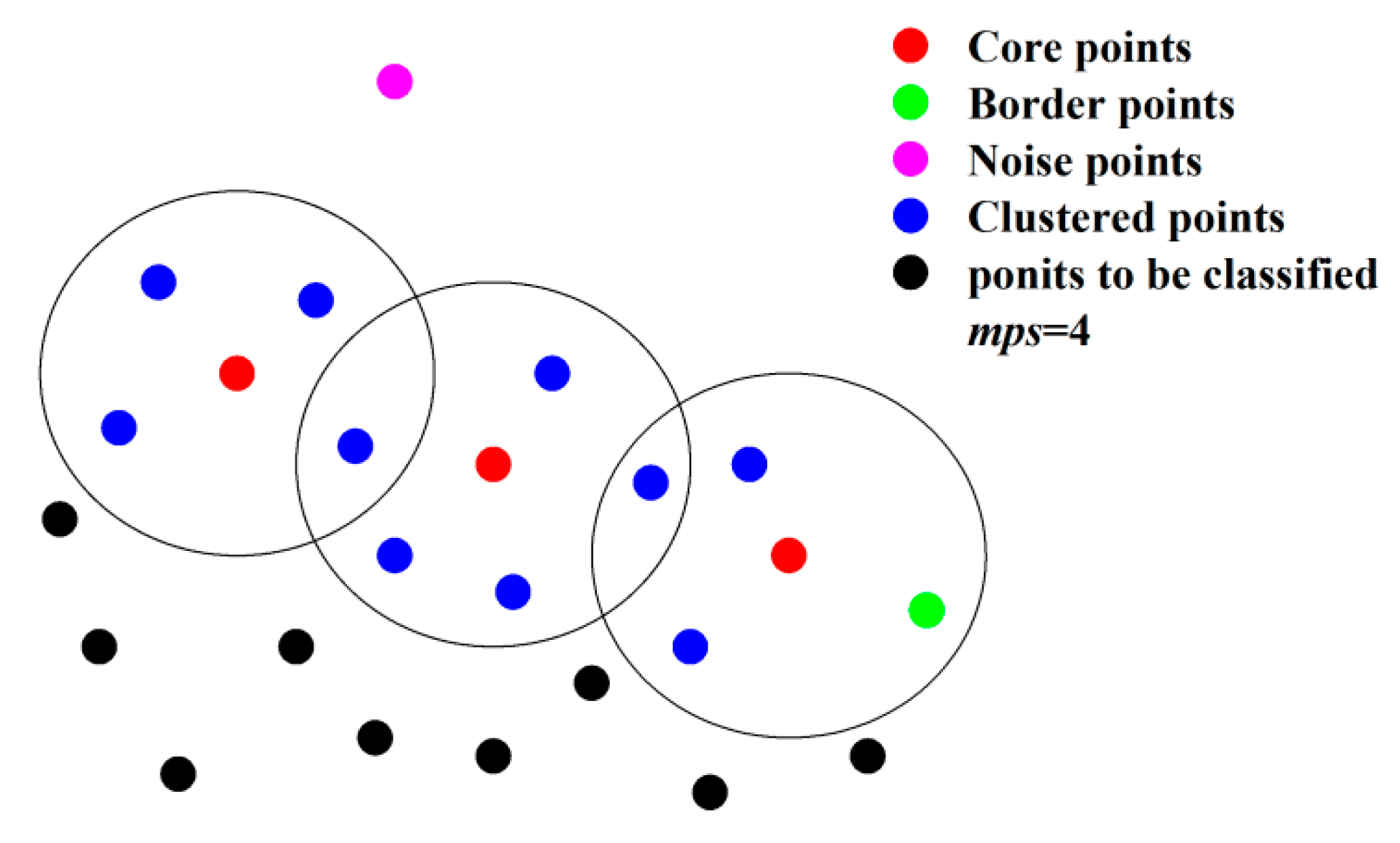
3.2. Mixing Matrix Estimation Based on Density Space Clustering

After the sparse enhancement of the mixed acoustic signals in the TF plane, the next stage is the estimation of the mixing matrix. Here, we can use a clustering algorithm to estimate the mixing matrix. The real and imaginary parts of X(t, f) in the TF plane are stacked into an array, and this array is used as the input for the clustering algorithm. Then, the output of the clustering algorithm is the mixing matrix estimation.

There are many kinds of clustering algorithms including system clustering, K-means clustering, birch clustering and density clustering. Among them, the density clustering algorithm represented by density-based spatial clustering of applications with noise (DBSCAN) can automatically determine the number of clusters according to the density of samples in space, which is suitable for data sets with arbitrary shapes. We consider the sample set C = (P₁, P₂, ..., P_C), the definitions of various sample points in the algorithm are shown in Figure 1, and the descriptions are as follows [22,23]:

(1)

Eps-neighborhood: for P ∈ C, the set of sample points contained in the hypersphere region with P as the center and Eps as the radius is called the Eps-neighborhood of P, i.e., $N_E(P)=\text{{}Q\in C\mid \mathrm{dist}(P,Q)\le \mathit{Eps}\text{}}$. Where dist(P, Q) is the distance between sample point P and Q in C.

(2)

Core point: for P ∈ C, if the number of sample points contained in N_E(P) is more than or equal to mps, i.e., $\mid N_E(P)\mid \ge \mathit{mps}$, P is called the core point of C.

(3)

Directly density reachable: for Q ∈ C, if $\mid N_E(P)\mid \ge \mathit{mps}$ and Q ∈ N_E(P), Q is directly density reachable from P.

(4)

Density reachable: for P₁, P₂, ..., P_C ∈ C, if P_c+1 is directly density reachable from P_c, where 1 ≤ c ≤ C−1, P_C is density reachable from P₁.

(5)

Boundary point: for Q ∈ C, if N_E(Q) < mps, N_E(P) ≥ mps and Q ∈ N_E(P), Q is the boundary point of C.

(6)

Noise point: for Q ∈ C, if Q does not belong to Eps-neighborhood of any core point, Q is the noise point of C.

The implementation process of mixing matrix estimation based on DBSCAN can be described as follows: Given the input parameter (Eps, mps), randomly select a data point (t, f) in the normalized data as the starting point. If (t, f) satisfies $\mid N_E\left(t,f\right)\mid \ge \mathit{mps}$, a cluster is formed when all density reachable sampling points belonging to the core point (t, f) are found. Then, the above action is repeated for all data points, and the data points without any cluster are regarded as noise points.

3.3. Source Signals Recovery Based on Compressed Sensing

3.3.1. Compressed Sensing

The essence of compressed sensing is an inverse linear problem, which aims to recover high-dimensional source signals from a small number of linear observation signals collected by sensors [24,25]. The compressed sensing model can be expressed as

$$\mathit{x}=\mathsf{\Phi }\mathit{s}$$

(11)

where x = [x(1),x(2),···,x(M1)]^T are the observed signals, $\mathsf{\Phi }\in {ℝ}^{M1\text{×}N1}$ is the measurement matrix with M₁ < N₁, s = [s(1),s(2),···,s(N1)]^T are the unknown sparse source signals. Then, the source signals can be recovered by solving the L₀ norm optimization problem:

$$\left\{\begin{array}{c}\widehat{\mathit{s}}=\arg \min \Vert \mathit{s}\Vert \\ \mathrm{s}.\mathrm{t}.\mathit{x}=\mathsf{\Phi }\mathit{s}\end{array}\right.$$

(12)

The L₀ norm optimization problem is usually solved by the orthogonal matching pursuit (OMP) algorithm [26].

3.3.2. Source Signals Recovery

The underdetermined blind source separation model of the mixed acoustic signals is the same as the compressed sensing model. Hence, the transformer acoustic signal can be recovered by constructing the compressed sensing model and using the OMP algorithm to solve Equation (11) [27].

Firstly, we select the mixed acoustic signals and sound source signals in the TF plane at a time frame t = 1 as the starting signal, i.e.,

X(f) = [X₁(f), X₂(f), ..., X_M1(f)]^T

(13)

S(f) = [S₁(f), S₂(f), ..., S_N1(f)]^T, f = 1,2,...,L

(14)

where L is the length of a time frame signal in the TF plane. Then We interleave X(f) and S(f) into vectors as follows:

X = [X₁(1), ..., X_M1(1), X₁(2), ..., X_M1(2), ..., X₁(L), ..., X_M1(L)]^T

(15)

S = [S₁(1), ..., S_N1(1), S₁(2), ..., S_N1(2), ..., S₁(L), ..., S_N1(L)]^T

(16)

Thus, the underdetermined blind source separation model of the mixed acoustic signals in Equation (4) can be expressed as

X = ΦS

(17)

$$\mathsf{\Phi }=\left[\begin{array}{cccc}\mathit{A}& \mathbf{0}& \cdots & \mathbf{0}\\ \mathbf{0}& \mathit{A}& \cdots & \mathbf{0}\\ ⋮& \text{…}& \ddots & ⋮\\ \mathbf{0}& \mathbf{0}& \cdots & \mathit{A}\end{array}\right]$$

(18)

where 0 is an M × N matrix of zeros. The measurement matrix estimation is obtained by using the mixing matrix estimation B instead of the mixing matrix A. So far, the compressed sensing model of the mixed acoustic signals has been established.

Then, the vector estimation $\widehat{\mathit{S}}$ is obtained by using the OMP algorithm to solve Equation (17), and N1 sound source signals estimation $\widehat{S}={\left[{\widehat{S}}_1{(f),\widehat{S}}_2(f),\dots {,\widehat{S}}_{N1}(f)\right]}^T$ at time frame t = 1 are split from the vector estimation by Equation (16).

Finally, the above action is repeated for each time frame signal in the TF plane and the recovery of the sound source signals are obtained by inverse short-time Fourier transform.

To sum up, the flowchart of the blind source separation method of transformer acoustic signal based on sparse component analysis is shown in Figure 2.

4. Simulation Analysis

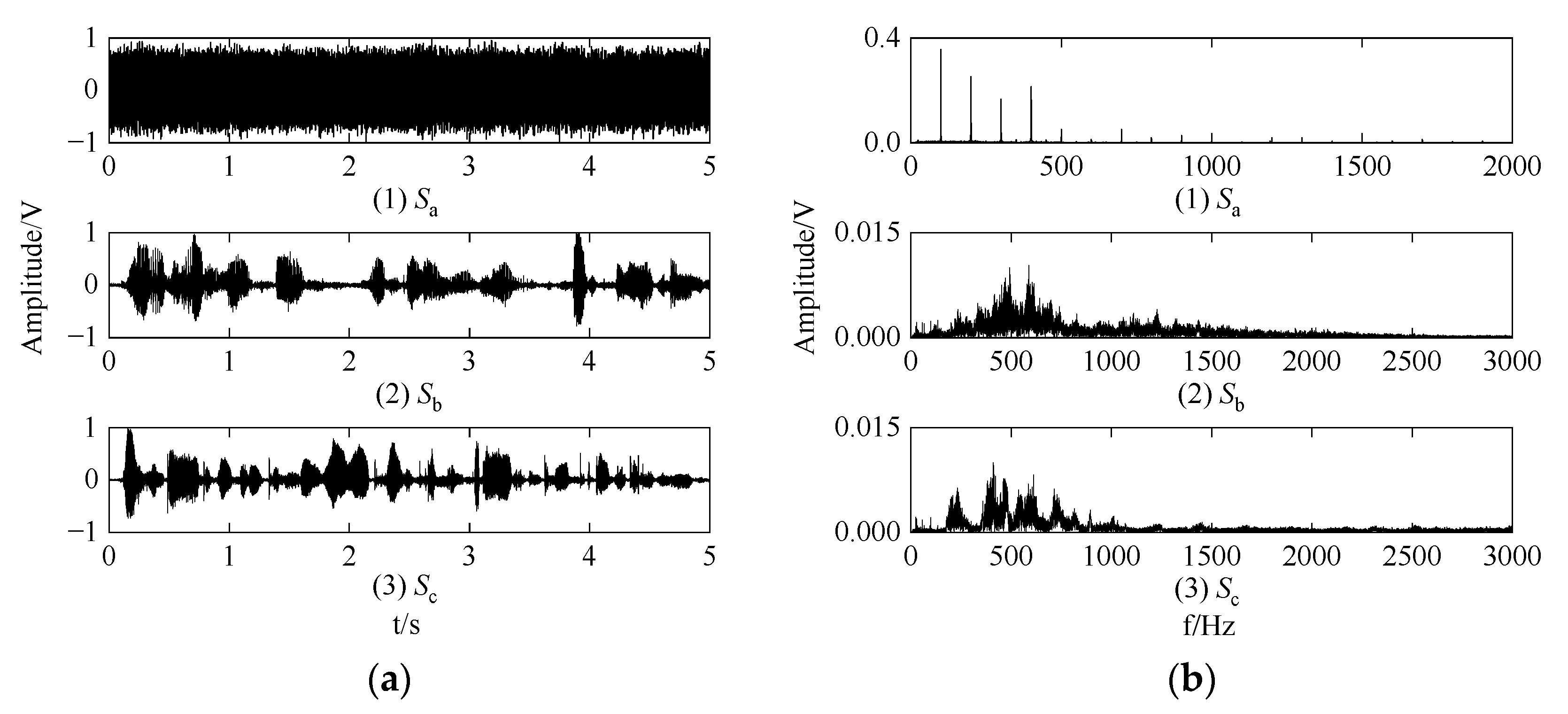
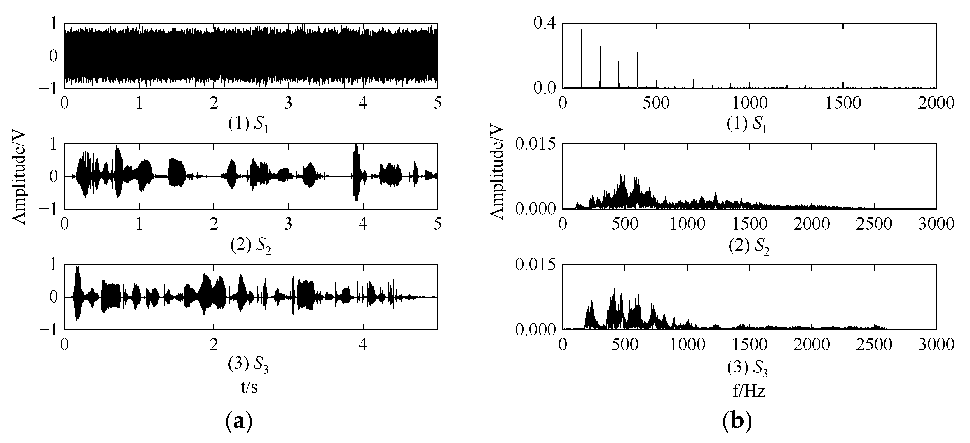
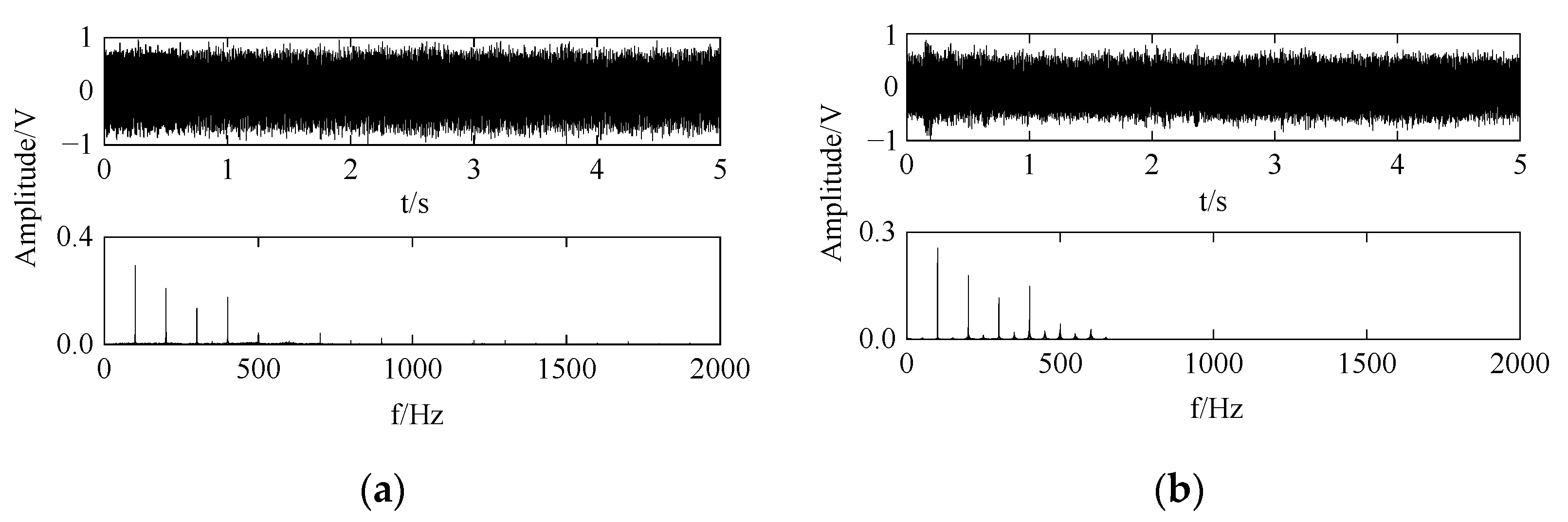
4.1. Simulation Signals

The dry-type transformer with model SCB 10-630/10 was taken as the simulation experimental object, the ATR2100 microphone was used as the acquisition device of the transformer acoustic signal, and the sound acquisition device was fully remotely controllable by a personal computer. The microphone was set 0.1 m away from the high voltage side of the transformer and 1 m away from the ground. The layout of the simulation experiment is shown in Figure 3, and a, b and c in Figure 3 are three phases on the high voltage side of the transformer, i.e., phase a, phase b and phase c. The transformer acoustic signal S₁ is collected through the microphone under the environment of 10 dB background noise, and two speech signals are randomly selected from the TIMIT as two interference signals S₂ and S₃. The sampling frequency of the signals is 16 kHz and the sampling time is 4 s.

Figure 4 shows waveforms and spectrums of three sound source signals of simulation, it can be seen from Figure 4 that the spectrum of the transformer acoustic signal is mainly distributed within 1000 Hz, mostly 100 Hz and higher order harmonics.

In practice, the mixed acoustic signals collected by acoustic sensors are generally formed by the random mixing of multiple sound source signals. Therefore, we randomly generate a mixing matrix:

$$\mathit{A}=\mathbf{ }\left[\begin{array}{ccc}-0.7660& 0.9848& 0.6691\\ 0.6428& 0.1737& 0.7431\end{array}\right]$$

(19)

Then, the mixed acoustic signals X(t) = [X₁(t),X₂(t)]^T is generated by Equation (1). Figure 5 shows waveforms and spectrums of the mixed acoustic signals of simulation. From Figure 5 it can be seen that the frequency components of the mixed acoustic signals are relatively complex, and there are low-frequency and high-frequency interferences with large amplitude in the spectrum range of 0–2000 Hz.

4.2. Simulation Experiment and Analysis

The mixed acoustic signals X(t) is transformed to TF domain by STFT. The parameters of STFT are set as: STFT size 1024, Hanning window as the weighting function and the overlap size of window 512.

Figure 6a shows a scatter diagram of the mixed acoustic signals in the time domain, the x-axis is the amplitude of X₁ and the y-axis is the amplitude of X₂ in the scatter diagram. Figure 6b shows the scatter diagram of the mixed sound signals X(t, f) in the TF domain, the x-axis is the amplitude of R{X₁(t, f)} and the y-axis is the amplitude of R{X₂(t, f)} in scatter diagram.

From Figure 6b it can be seen that the mixed acoustic signals in the TF domain show approximate sparsity and linear clustering characteristics, but they still cannot meet the sparsity requirements of SCA. Therefore, the SSPs X_SSP(t, f) of the mixed acoustic signals in the TF domain are extracted by using the single-source-point identification method and the parameter of the SSP identification method is set to β = 0.02 [19]. Then, the normalized data X_nor(t, f) are obtained by normalizing X_SSP(t, f). Figure 7 shows scatter diagrams of the real part of the SSPs and normalized data, respectively.

As shown in Figure 7, the mixed acoustic signals have obvious sparsity and clustering characteristics after SSP identification and normalization. The normalized data are clustered using DBSCAN algorithm, The parameters of DBSCAN algorithm are: Eps = 0.07, mps = 10. The mixing matrix estimation and its error are

$$\mathit{B}=\left[\begin{array}{ccc}-0.7713& 0.9841& 0.6623\\ 0.6411& 0.1775& 0.742\end{array}\right]$$

(20)

and

$$\mathit{A}-\mathit{B}=\left[\begin{array}{ccc}0.0053& 0.0007& 0.0068\\ 0.0017& -0.0038& -0.0061\end{array}\right]$$

(21)

It can be seen from Equation (21) that the number of source signals and the mixing matrix can be accurately estimated by the DBSCAN algorithm. Then three sound source signals are recovered by constructing the compressed sensing model and using the OMP algorithm to solve Equation (17). As shown in Figure 8, the waveforms of three recovered signals are similar to that of three source signals, and the three recovered signals, in turn, are transformer acoustic signal S_a, voice signal S_b, and voice signal S_c. The low-frequency and high-frequency interference signals in the mixed acoustic signals are eliminated, and the frequency characteristic of the transformer acoustic signal is preserved completely by the transformer recovered signal.

4.3. Comparison with Other Methods

In order to further verify the denoising effect of the proposed method, two typical denoising methods of the transformer acoustic signal are used to denoise the mixed acoustic signals of simulation respectively, and their denoising performance is compared with the proposed method. Method 1 and method 2 are respectively potential function-SCA method in [1] and the WPT-comb filter method in [3]. The denoising results of the two methods are shown in Figure 9.

Two evaluation indexes, normalized correlation coefficient (NCC) and signal–noise ratio (SNR), are introduced to evaluate the denoising effect of the three methods. They are defined as follows:

NCC is used to measure the waveform similarity between the source signal and the recovered signal, which is defined as

$$\mathrm{NCC}=\frac{{\sum }_{t=1}^T\left|S_n{(t)\widehat{S}}_n(t)\right|}{\sqrt{{\sum }_{t=1}^T{S}_n^2(t){\sum }_{t=1}^T{\widehat{S}}_n^2(t)}}$$

(22)

where S_n(t) and ${\widehat{S}}_n\left(t\right)$ are respectively the nth source signal and its recovered signal; T is the length of the signal. The closer NCC is to 1, the closer the recovered signal is to the source signal.

SNR is used to measure noise content in the recovered signal, which is defined as

$$\mathrm{SNR}=10\lg \left(\frac{{{\displaystyle \sum }}_{\mathrm{t}=1}^{\mathrm{T}}{S}_n^2(t)}{{\sum }_{t=1}^T{\left[S_n{(t)-\widehat{S}}_n(t)\right]}^2}\right)$$

(23)

The higher the SNR, the less the noise content of the recovered signal. The evaluation indexes of the denoising effect of the three denoising methods are shown in

Table 2. Evaluation indexes of denoising effect of the three methods.

Evaluation Index	Proposed Method	Method 1	Method 2
NCC(S1, Sa)	0.9941	0.9648	0.8413
SNR(S1, Sa)/dB	20.1829	13.8940	4.9459

.

The following conclusions can be drawn by analyzing the results of Figure 8 and Figure 9 and Table 2:

Compared to the denoising results and the evaluation indexes of the denoising effect of the three methods, it can be seen that the proposed method has the best denoising effect, and the waveform and spectrum of the transformer recovered signal are basically the same as the original signal, with the minimum error.

Compared with method one, the sparsity and linear clustering characteristics of the mixed acoustic signals are enhanced by SSP identification in the proposed method, and the accuracy and robustness of the blind source separation method are improved.

The 50 Hz frequency doubling parts of the interference signals will be retained by the comb filter when method two is used to denoise the transformer acoustic signal. The transformer recovery signal has been mixed with some interference signals, resulting in the generation of frequency components that do not originally exist in the transformer, which affects the accuracy of subsequent fault diagnosis.

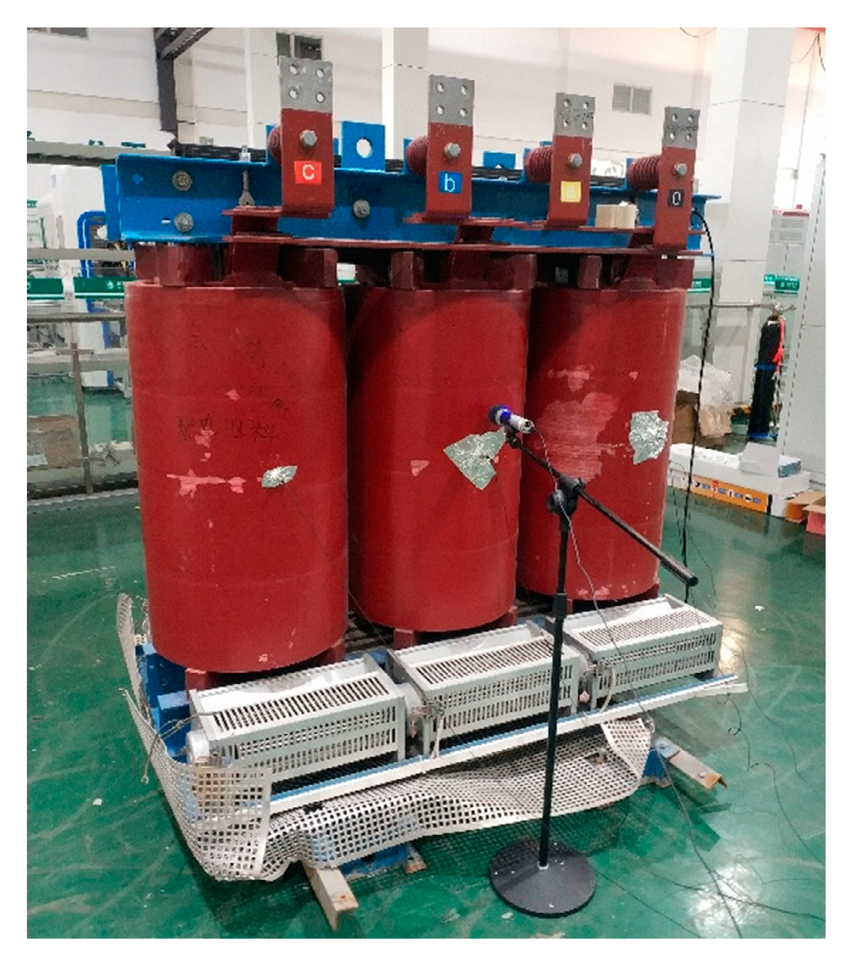
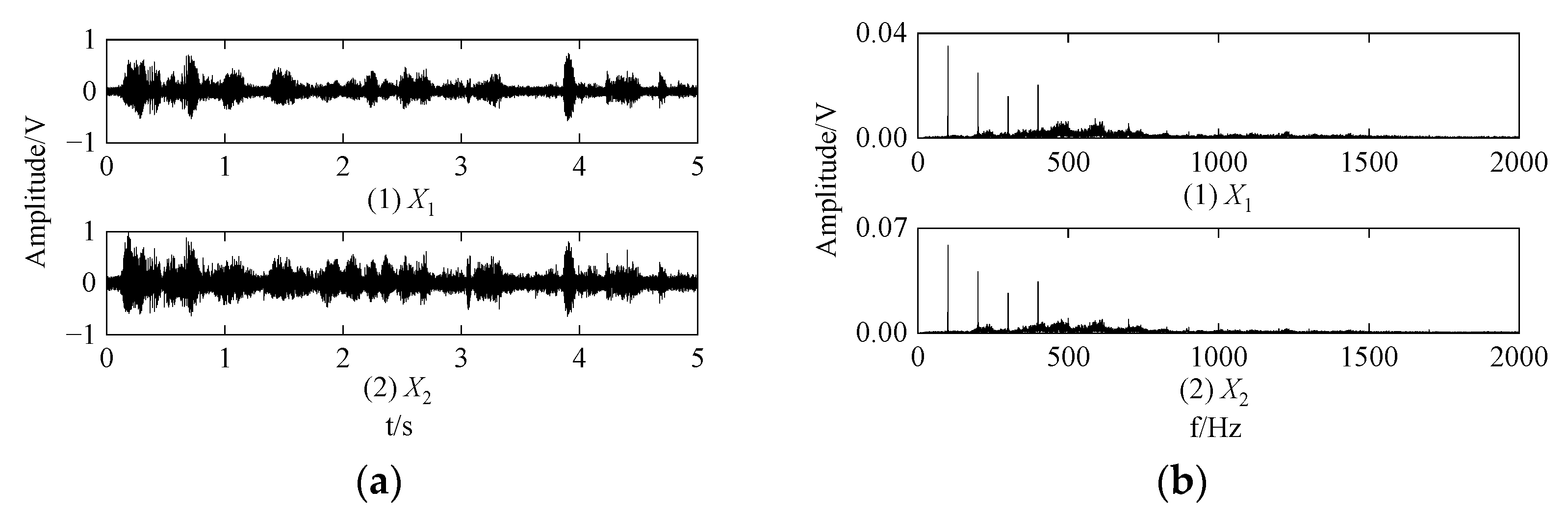
5. Experimental Analysis

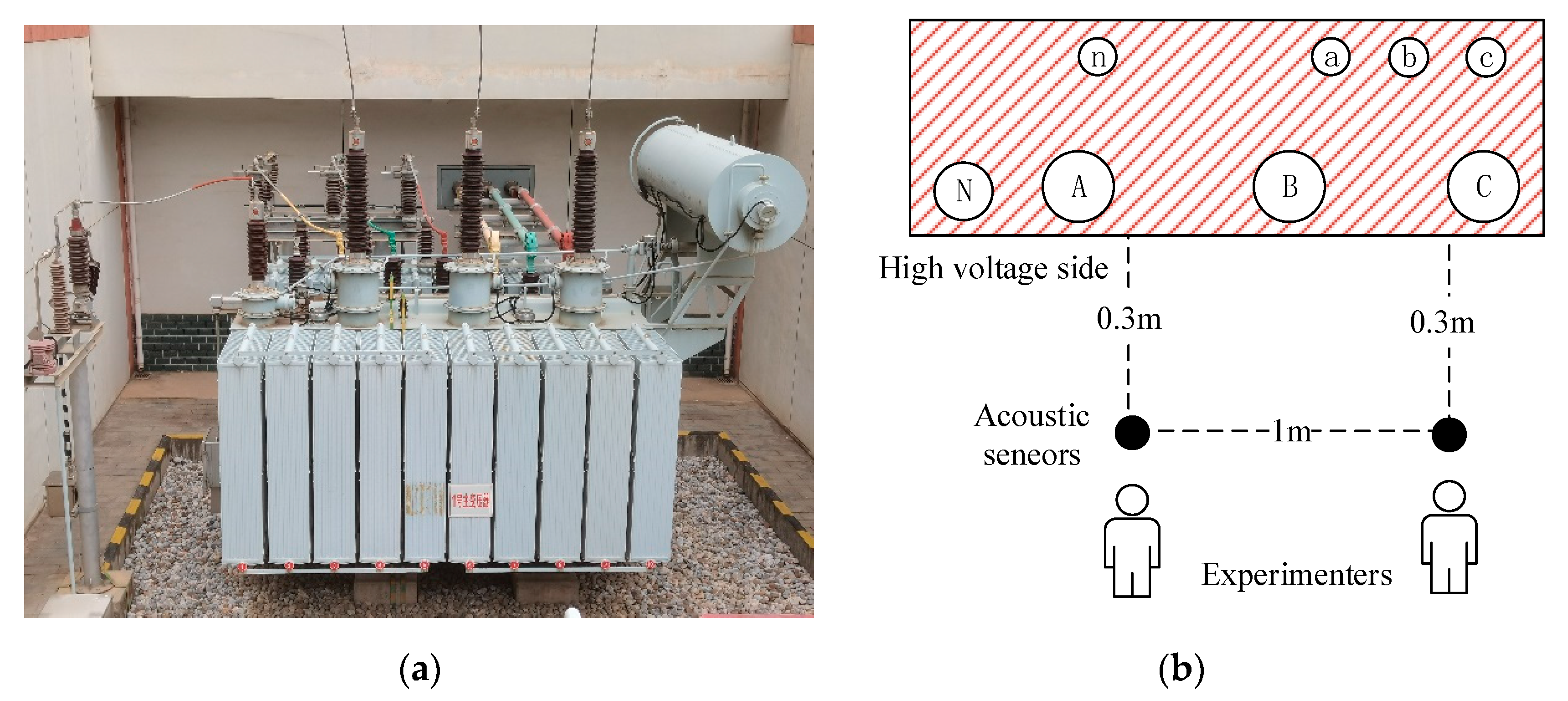
5.1. Experimental Setup

In order to verify the effectiveness of the proposed method in processing the measured transformer acoustic signal, the experiment was set in a 110 kV substation. The experiment object is the main transformer of the substation. The parameters of the transformer are: three phases oil-immersed transformer, the rated capacity is 50 MVA, the rated frequency is 50 Hz, and the rated voltage is (121 ± 8 × 1.25%)/10.5 kV. Firewalls are installed on both sides of the transformer, and cooling fans are installed on the left side of the transformer.

According to IEC 60651 standard, COINV-INV9206 acoustic sensors and NI-9232 data acquisition card were selected to form a sound acquisition system, and the sensor and acquisition card is connected through the BNC interface. The sound acquisition system is fully remotely controllable by a personal computer. The parameters of the acoustic sensor are: the length of the acoustic sensor is 85 mm, the nominal sensitivity is 50 mV/Pa, the frequency range is 20 Hz~20 kHz, the dynamic range is 20~146 dB, the working temperature range is −35~80 °C, the temperature coefficient is −0.008 dB/°C. The parameters of the data acquisition card are: the number of analog input channels is 4, the maximum sampling rate is 102.4 kHz, and the analog input voltage range is −30~30 V. The sampling frequency of the sound acquisition system is set to 48 kHz. The acoustic sensors were arranged according to GB/T 1094.10-2003 standard: two acoustic sensors were set 0.3 m away from the front box of the transformer, 1.5 m away from the ground, and the distance between the two sensors was set at 1 m. The physical diagram and experiment schematic diagram of the transformer are shown in Figure 10.

Two experimental assistants located on each side of the sensor began talking to each other as soon as the experiment started, and two mixed acoustic signals in the substation were collected by the sensors are shown in Figure 11. Then, the transformer acoustic signal in the substation was collected by any sensor as the reference signal, waveform and spectrum of the reference signal are shown in Figure 12.

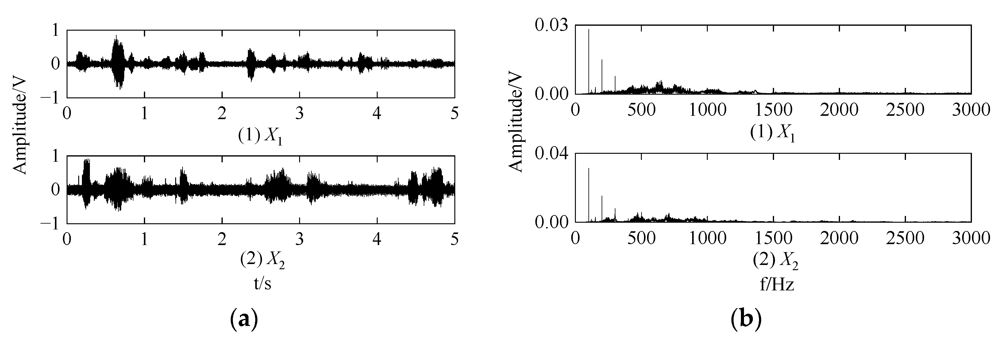
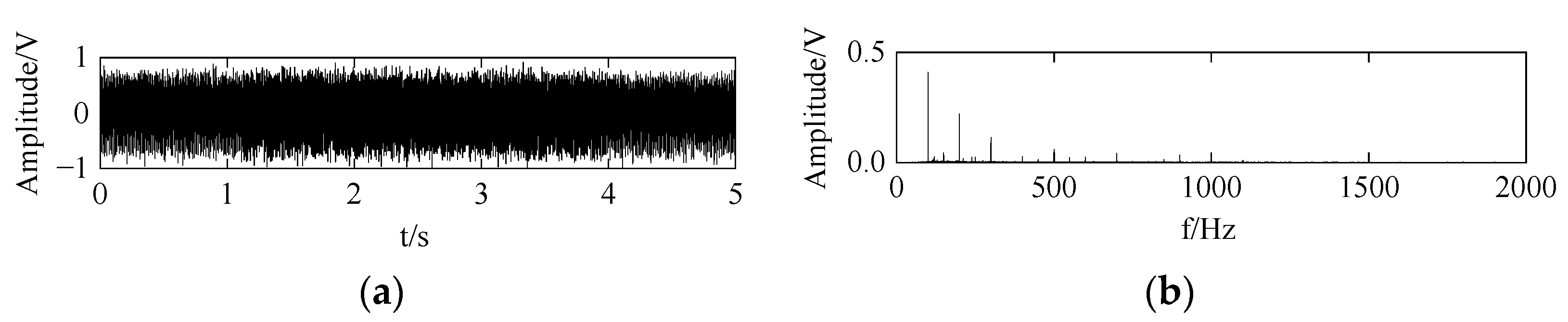
5.2. Experimental Results and Analysis

The recovered signals are separated from two mixed acoustic signals by using the presented method. Three recovered signals, in turn, are transformer acoustic signal S_a, voice signal S_b, and voice signal S_c. Figure 13 shows the waveforms and spectrums of the recovered signals. The separation results show that the waveform of the transformer recovery signal S_a is roughly the same as that of the reference signal, and the main frequency peaks in the two signal spectrums correspond to each other one by one.

The normalized correlation coefficient and signal–noise ratio of transformer recovery signal and reference signal are shown in

Table 3. Evaluation indexes of the proposed method separation effect.

Evaluation Index	(X1, Sa)	(X2, Sa)	(S1, Sa)
NCC	0.4927	0.6472	0.9254
SNR/dB	0.7885	1.6663	8.8580

. From Table 2 and Table 3, it can be seen that the NCC and SNR of the transformer recovery signal in the experiment are smaller than those in the simulation because there is a lot of background noise including the sound of the wind, the reflection of the substation buildings walls and transformer tanks in the substation, which reduces the accuracy of the proposed method. Although the substation environment has a great impact on signal separation, the NCC and SNR of the transformer recovered signal in the experiment can reach 0.9254 and 8.8580 respectively. Besides, compared with the mixed acoustic signals, the evaluation indexes of the transformer recovery signal have been significantly improved. In other words, the separation of the transformer acoustic signal is not affected by the background noise.

The experimental results show that the transformer acoustic signal can be effectively separated from the measured mixed acoustic signals by the proposed method under the condition of underdetermination, and the frequency characteristics of the transformer acoustic signal are well preserved.

6. Conclusions

Aiming at the problems of useless signal interference in transformer acoustic signals, a blind source separation method of transformer acoustic signals based on sparse component analysis is proposed in this paper. Through the analysis of simulation and experimental results, it can be seen that the proposed method can effectively separate the transformer acoustic signal from the mixed acoustic signals and can protect the spectrum information in the transformer acoustic signal. Compared with the existing transformer acoustic signal denoising methods, the proposed method has strong applicability, small denoising result error, and small waveform and spectrum distortion. The method also has limitations, such as the method needs to use multiple sensors, which is not suitable for the case of a single sensor; The linear instantaneous mixed model used in this paper may not be applicable to convolution mixed model and nonlinear mixed model, which is the focus of the next step of the method.

References

1. Zou, L.; Guo, Y.K.; Liu, H.; Zhang, L.; Zhao, T. A Method of Abnormal States Detection Based on Adaptive Extraction of Transformer Vibro-Acoustic Signals. Energies 2017, 10, 2076. [Google Scholar] [CrossRef]
2. Adnan, S.; Matej, K.; Igor, K. Vibro-Acoustic Methods in the Condition Assessment of Power Transformers: A Survey. IEEE Access 2019, 7, 83915–83931. [Google Scholar]
3. Liu, Y.P.; Wang, B.W.; Yue, H.T.; Gao, F.; Han, S.; Luo, S.H.; Zhang, C.C. Identification of Transformer Bias Voiceprint Based on 50Hz Frequency Multiplication Cepstrum Coefficients and Gated Recurrent Unit. Proc. CSEE 2020, 40, 4681–4694. [Google Scholar]
4. Pan, L.L.; Zhao, S.T.; Li, B.S. Electrical equipment fault diagnosis based on acoustic wave signal analysis. Electr. Power Autom. Equip. 2009, 29, 87–90. [Google Scholar]
5. Shams, M.A.; Anis, H.I.; El-Shahat, M. Denoising of heavily contaminated partial discharge signals in high-voltage cables using maximal overlap discrete wavelet transform. Energies 2021, 14, 6540. [Google Scholar] [CrossRef]
6. Wu, X.W.; Zhou, N.G.; Pei, C.M.; Hu, S.; Huang, T.; Ying, L.M. Separation methodology of audible noises of UHV AC substations. High Volt. Eng. 2016, 42, 2625–2632. [Google Scholar]
7. Liu, Z.Y.; Liu, Z.Y.; Fan, H.M. Study on signal de-noising of high voltage cable partial discharge based on EMD-ICA. Power Syst. Prot. Control 2018, 46, 83–87. [Google Scholar]
8. Chan, J.C.; Hui, M.; Saha, T.K.; Ekanayakel, C. Self-adaptive partial discharge signal denoising based on ensemble empirical mode decomposition and automatic morphological thresholding. IEEE Trans. Dielectr. Electr. Insul. 2014, 21, 294–303. [Google Scholar] [CrossRef]
9. Hao, L.; Lewin, P.L.; Hunter, J.A.; Swaffielf, D.J.; Contin, A.; Walton, C.; MIchel, M. Discrimination of multiple PD sources using wavelet decomposition and principal component analysis. IEEE Trans. Dielectrics Electr. Insul. 2011, 18, 1702–1711. [Google Scholar] [CrossRef]
10. Alvarez, F.; Garnacho, F.; Ortego, J.; Sanchez-Uran, M.A. A clustering technique for partial discharge and noise sources identifification in power cables by means of waveform parameters. IEEE Trans. Dielectr. Electr. Insul. 2016, 23, 469–481. [Google Scholar] [CrossRef]
11. Wang, Y.B.; Chang, D.C.; Qin, S.R.; Fan, Y.H.; Mu, H.B.; Zhang, G.J. Separating multi-source partial discharge signals using linear prediction analysis and isolation forest algorithm. IEEE Trans. Instrum. Meas. 2020, 69, 2734–2742. [Google Scholar] [CrossRef]
12. Han, S.; Gao, F.; Wang, B.W.; Liu, Y.P.; Wang, K.; Wu, D.; Zhang, C.C. Audible sound identification of on load tap changer based on mel spectrum filtering and CNN. Power Syst. Technol. 2021, 45, 3609–3617. [Google Scholar]
13. Stergiadis, C.; Kostaridou, V.D.; Klados, M.A. Which BSS method separates better the EEG Signals? A comparison of five different algorithms. Biomed. Signal Process. Control 2022, 72, 103292. [Google Scholar] [CrossRef]
14. Dorothea, K.; Ramon, F.A.; Eugen, H.; Reinhold, O. Independent component analysis and time-frequency masking for speech recognition in multitalker conditions. EURASIP J. Audio Speech Music Process. 2010, 1, 1–13. [Google Scholar] [CrossRef]
15. Reju, V.G.; Koh, S.N.; Soon, I.Y. An algorithm for mixing matrix estimation in instantaneous blind source separation. Signal Process. 2009, 89, 1762–1773. [Google Scholar] [CrossRef]
16. Guo, J.; Ji, S.C.; Shen, Q.; Zhu, L.Y.; Ou, X.B.; Du, L.M. Blind source separation technology for the detection of transformer fault based on vibration method. Trans. China Electrotech. Soc. 2017, 27, 68–78. [Google Scholar]
17. Lin, S.F.; Li, Y.; Tang, B.; Fu, Y.; Li, D.D. System harmonic impedance estimation based on improved fastica and partial least squares. Power Syst. Technol. 2018, 42, 308–314. [Google Scholar]
18. Zhou, D.X.; Wang, F.H.; Dang, X.J.; Zhang, X.; Liu, S.G. Blind Separation of UHV Power Transformer Acoustic Signal Preprocessing Based on Sparse Representation Theory. Power Syst. Technol. 2020, 44, 3139–3148. [Google Scholar]
19. Bofill, P.; Zibulevsky, M. Underdetermined blind source separation using sparse representations. Signal Process. 2001, 81, 2353–2362. [Google Scholar] [CrossRef]
20. Bofill, P. Underdetermined blind separation of delayed sound sources in the frequency domain. Neurocomputing 2003, 55, 627–641. [Google Scholar] [CrossRef]
21. Li, M.Z.; Li, S.M.; Lu, J.T. Underdetermined blind source separation based on density peak clustering for gear fault identification. J. Aerosp. Power 2022, 37, 1010–1019. [Google Scholar]
22. Li, X.; Zhang, P.; Zhu, G. DBSCAN clustering algorithms for non-uniform density data and its application in urban rail passenger aggregation distribution. Energies 2019, 12, 3722. [Google Scholar] [CrossRef]
23. Nooshin, H.; Hamid, S. A fast DBSCAN algorithm for big data based on efficient density calculation. Expert Syst. Appl. 2022, 203, 117501. [Google Scholar]
24. Donoho, D.L. Compressed sensing. IEEE Trans. Inf. Theory 2006, 52, 1289–1306. [Google Scholar] [CrossRef]
25. Ruiz, M.; Montalvo, I. Electrical faults signals restoring based on compressed sensing techniques. Energies 2020, 13, 2121. [Google Scholar] [CrossRef]
26. Zhang, Y.J.; Zhang, S.Z.; Qi, R. Compressed sensing Construction for Underdetermined Source Separation. Circuits Syst. Signal Process. 2017, 36, 4741–4755. [Google Scholar] [CrossRef]
27. Zhao, H.F.; Zhang, Y.; Li, S.Z. Undetermined blind source separation and feature extraction of penetration overload signals. Chin. J. Sci. Instrum. 2019, 40, 208–218. [Google Scholar]
Figure 1. Clustering principle of the DBSCAN algorithm.
Energies 15 06017 g001
Figure 2. The Flowchart of the proposed method.
Energies 15 06017 g002
Figure 3. Layout of simulation experiment.
Energies 15 06017 g003
Figure 4. Waveforms and spectrums of the source signals; ((a): waveforms; (b): spectrums).
Energies 15 06017 g004
Figure 5. Waveforms and spectrums of the mixed acoustic signals; ((a): waveforms; (b): spectrums).
Energies 15 06017 g005
Figure 6. Scatter diagram of the mixed acoustic signals in time domain and time-frequency domain; ((a): time domain; (b): time-frequency domain).
Energies 15 06017 g006
Figure 7. Scatter diagram of the real part of the SSPs and normalized data; ((a): the real part of the SSPs; (b): the real part of the normalized data).
Energies 15 06017 g007
Figure 8. Waveforms and spectrums of three recovered signals of simulation; ((a): waveforms; (b): spectrums).
Energies 15 06017 g008
Figure 9. Waveforms and spectrums of the transformer recovered signal using the two methods; ((a): method 1; (b): method 2).
Energies 15 06017 g009
Figure 10. Physical diagram and experiment schematic diagram of the transformer; ((a): power transformer, three phases, 50 MVA, 50 Hz; (b): experiment schematic diagram).
Energies 15 06017 g010
Figure 11. Waveforms and spectrums of the mixed acoustic signals in the substation; ((a): waveform; (b): spectrum).
Energies 15 06017 g011
Figure 12. Waveform and spectrum of the reference signal in the substation; ((a): waveform; (b): spectrum).
Energies 15 06017 g012
Figure 13. Waveforms and spectrums of the recovered signals in the substation; ((a): waveform; (b): spectrum).
Energies 15 06017 g013