A Method for Evaluating the Dominant Seepage Channel of Water Flooding in Layered Sandstone Reservoir

Abstract

A method for evaluating the dominant seepage channel (DSC) water flooding in a layered sandstone reservoir is proposed and applied in an oilfield based on the water-cut derivative. The water-cut derivative curve of the reservoir with DSC shows double peaks. Therefore, based on the analysis of geology and production characteristics, the evaluation method of DSC is established. The evaluation index is proposed to quantitatively characterize the development degree of DSC and determine its distribution in a water-flooding reservoir. The test data validate that the proposed method can not only accurately determine the DSC and quantitatively evaluate its development degree, but also show its dynamic change. This method will be a powerful guide for water controlling and oil stabilizing in the adjustment stage of sandstone reservoirs.

1. Introduction

The concept of the dominant seepage channel (DSC) was first proposed by Shengli Oilfield in the 1980s [1]. Zhao et al. [2] believed that the pores generated by the erosion of injection water were secondary ones, and those with a pore size over 30 μm were called DSCs. This is the first time that a clear boundary has been given for a DSC. Subsequently, Jiang H. [3], Zeng et al. [4], and Meng et al. [5] conducted a large number of experimental studies of the existence, formation, and application of the DSC concept, and determined its definition by combining seepage theory and Darcy’s law. Liu and Liang [6], Deng et al. [7], and Wu and Li [8] established the classification criteria of the DSC by means of microscopic analysis, tracer monitoring, and well test analysis.

The formation of the DSC is the result of the joint action of geological, fluidic, and production factors. It is dynamic and difficult to identify. Therefore, rational use of scientific and effective methods is the key to identify the DSCs in reservoirs. In 1995, Chan K. [9] firstly proposed a log–log coordinate curve of water–oil ratio/gas–oil ratio and its derivative with respect to time to identify bottom water coning/gas channeling, hyperpermeability bands, interlayer channeling, and hyperpermeability channels around wells. This method was called the Chan plot. Yortsos et al. [10] discussed the practical feasibility of the Chan plot. Numerical simulation and seepage mechanics theory were used to analyze the double logarithm curves of reservoirs with different permeability distributions under different water flooding modes. The results showed that the slope of the curve at the later stage of the double logarithm coordinates may be related to the well operating mode and relative permeability. In 2002, Wang et al. [11] analyzed its formation mechanism and summarized five effective identification methods for it according to the abnormal response of logging data in the injection profile. In 2007, Shi L. [12] proposed a method to identify the DSC by inter-wells tracing technology. In 2011, Izgec and Kabir [13] proposed an improved Hall curve analysis, which can be used to identify and characterize the DSCs between injection-production wells. In 2013, Oftedal et al. [14] first used distributed temperature sensing (DTS) technology along with production logging tools and water flow logging to detect the location of hyperosmotic zones in fractured wells based on inter-well connectivity analysis. In 2014, Hao J. [15] proposed a new combined parameter, the dimensionless pressure index, to identify the DSC by considering the dynamic change in reservoir permeability in the process of water flooding. In 2015, Huang et al. [16] established the DSC model and accurately identified the DSC in complex fault-block oilfields by combining it with mathematical methods, such as the hierarchical structure analysis method, construction of judgment matrix, calculation of weight, and consistency judgment. Ding et al. [17] proposed an integrated analysis method to characterize DSC and its development levels in water flooding reservoirs, and then used logical analysis theory to screen the static and dynamic parameters most relevant to the DSC. In 2019, Alotaibi [18] further studied the practical application of the Chan plot by using the pressure transient analysis (PTA) of horizontal wells. The results showed that PTA data played an important supporting role in identifying the DSC. In 2019, Gu W. [19] proposed a quantitative evaluation model for the DSC in loose sandstone reservoirs based on hierarchical analysis and the gray correlation method. In 2021, Lu C. et al. [20] proposed a method with a convolutional neural network to construct a classification model for the identification of the DSC. Ma R. et al. [21] have shown a correction mathematical model and correction workflow for PTA to identify DSC in a stratified carbonate reservoir. Fu et al. [22] proposed modified capacitance–resistance models based on the work of previous researchers [23,24,25,26,27,28,29,30] to study inter-well conductivities between the injector and producer. The application results indicated that the method was useful. It is helpful to identify the DSC.

It can be seen that the current research on the identification method of DSC is generally limited to the independent use of a single technology. Only by using the static and dynamic data of the studied area can the results of multiple DSC identification methods be verified with one other. The DSC can also be more accurately identified and described. This paper proposes a comprehensive evaluation method of the DSCs in layered sandstone reservoirs. On the basis of geology and production analysis, the quantitative evaluation index of a water flooding reservoir is proposed. The evaluation charts are also formed. This work can be used to determine the DSC distribution of water flooding in a layered sandstone reservoir.

2. Methods

2.1. Water-Cut Derivative Characteristics of a Reservoir with DSC

2.1.1. Curve Feature of Water-Cut

The DSC is formed in the heterogeneous reservoir under the condition of long-term water flooding. In a real oil reservoir, there are many different shapes of DSC. In order to reduce the interference caused by the shapes in this study, the DSC is simplified in the ideal model. Two reservoir numerical models with one injection well and one production well are established. The fixed injection rate is set in the former, and the fixed bottomhole flow pressure is set in the latter. The high permeability zone is set on the main flowline of injection and production wells in the first model to simulate the DSC. The other model is homogeneous without DSC. The variations of water-cut under the condition of DSC and non-DSC are simulated, respectively. Dimensionless time t_D, shown in Equation (1), and the water-cut derivative f_w′, shown in Equation (2), are introduced. The relation curve of these two parameters from the two models is shown in Figure 1a. Equations (1) and (2) are as follows:

$$t_D=\frac{q_{i}t}{A\Phi h}$$

(1)

$$f_w^{\prime }=\frac{d{f}_w}{d\left({\ln t}_D\right)}=t_D\frac{d{f}_w}{{dt}_D}$$

(2)

where, t_D is dimensionless time; q_i is production rate; t is production time; A is reservoir area; $\Phi$ is porosity; h is reservoir thickness; $f_w^{\prime }$ is the water-cut derivative; $f_w^{}$ is water-cut.

Through comparative analysis, it can be seen that the water-cut derivative curve with DSC shows double peaks, while the curve without DSC shows single peak. They reflect different flow processes of injected water. In the model with DSC, the first peak indicates the injected water reaching the production well along the DSC. It represents the influence of the DSC on the water-cut derivative. The second peak represents the injected water reaching the production well along non-DSCs. It reflects the influence of reservoir physical properties on the water-cut derivative in non-DSC regions. In the model without DSC, the front of the injected water is relatively homogeneous in that it shows only one peak in the water-cut derivative curve. Therefore, the DSC can be characterized by the derivative curve of a water-cut, and then it can be preliminarily identified by the curve. The water-cut and derivative curves of production wells during water flooding in the reservoirs with DSCs are divided into five stages (Figure 1a). The saturation distribution of injected water corresponding to the five stages is shown in Figure 1b. These stages are as follows:

Stage I—The injected water does not break through to the production well, and the water-cut remains unchanged;

Stage II—Starts from the first trough to the first peak when the injected water breaks through the DSC to the production well for the first time. The rising rate of the water-cut gradually increases, and the derivative curve shows upward trend;

Stage III—After the injected water breaks through the DSC to the well for the first time, a local stable oil–water interface is formed, and the water-cut derivative decreases;

Stage IV–Starts from the second trough to the peak when the injected water floods along the non-DSC to the production well. The rising rate of the water-cut gradually increases;

Stage V—After the injection water along the non-DSC breaks through the well twice, a stable oil–water interface is formed. The water-cut derivative decreases.

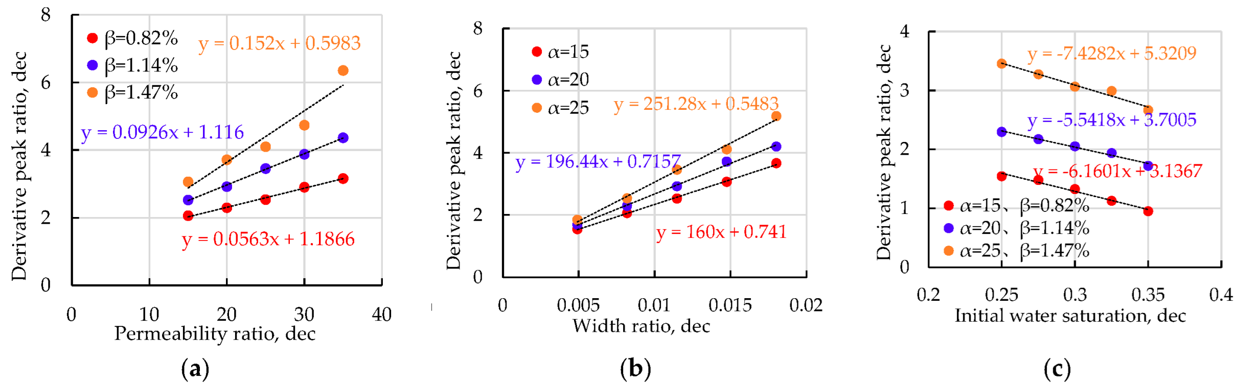
2.1.2. Relation of Feature Points in Derivative Curve

The coordinate ratio of the first and second feature points is taken as the studied object. The derivative peak ratio M, time ratio N, permeability ratio α, width ratio β of the DSC, and the initial water saturation S_wi of the reservoir are studied. Set the ratio of the two peaks in the derivative curve to be M and the times to be N, and then set the ratio of permeability K₁ of DSC to the permeability K of non-DSC to be α, and then set the ratio of equivalent width w of the DSC to total equivalent width a of the reservoir to be β, i.e., α and β are intermediate parameters in this study. There is one point that needs to be noted. The parameters w and a in Equation (6) are used in the model but are not needed in the application. In the model, we need to set a DSC with a specific size to determine the production performance in different stages. When a is given in the model, w can be calculated by β. The value range of β refers to the fractured reservoirs. Actually, these two parameters are hard to obtain in a real reservoir.

$$M=\frac{f_{w max1}^{\prime }}{f_{w max2}^{\prime }}$$

(3)

$$N=\frac{t_{D1}}{t_{D2}}$$

(4)

$$\alpha =\frac{K_1}{K}$$

(5)

$$\beta =\frac{w}{a}$$

(6)

where $f_{w max1}^{\prime } \mathrm{and} f_{w max2}^{\prime }$ are the derivative peaks of the water-cut corresponding to the first and second feature points, respectively, dec; M is derivative peak ratio, dec; $t_{D1}$ and $t_{D2 }$ are dimensionless time corresponding to the first and second feature points, respectively, dec; N is the time ratio, dec; $K_1$ is the permeability of DSC, mD; $K$ is the permeability of non-DSC, mD; $\alpha$ is the permeability ratio, dec; $w$ is the equivalent width of DSC, m; $a$ is the total equivalent width of reservoir, m; $\beta$ is the width ratio, dec.

A numerical simulation model is established to study the relationship between M, N, α, β, and S_wi. The results are shown in Figure 2 and Figure 3. Here, M has a linear relationship with α, β, and S_wi. The M increases with α, which represents the permeability difference. The β decreases with the increase in S_wi, which is closely related to the water-cut. It indicates that the DSC is more obvious in the reservoir with serious heterogeneity. Here, N is a power function with α, β, and S_wi.

2.2. Evaluation Index and Classification Criteria

During water flooding in the reservoir with DSCs, the produced water can be divided into two parts, namely water flowing into production wells along a DSC, and water flowing along a non-DSC. Combined with Darcy’s law and the established DSC model, two components of produced water volume are listed as follows:

$$q_{w1}=\frac{K_1{K}_{rw}\left(S_w\right)}{{\mu }_w}wh\frac{dP}{dx}$$

(7)

$$q_{w2}=\frac{K{K}_{rw}\left(S_w\right)}{{\mu }_w}\left(a-w\right)h\frac{dP}{dx}$$

(8)

where q_w1 is the amount of water flowing into the production well along the DSC, m³; q_w2 is the amount of water flowing into the production well along the non-DSC, m³; K_rw is the relative permeability of water phase; S_w is water saturation; μ_w is water viscosity, mPa·s; dp/dx is the pressure gradient, MPa/m.

In order to quantitatively evaluate the DSC, α and β are selected to establish the evaluation index of DSC, F_wcr.

$$F_{\mathit{wcr}}=\frac{q_{w1}}{q_{w1}+q_{w2}}=\frac{\frac{K_1{K}_{rw}\left(S_w\right)}{{\mu }_w}wh\frac{dP}{dx}}{\frac{K_1{K}_{rw}\left(S_w\right)}{{\mu }_w}wh\frac{dP}{dx}+\frac{K{K}_{rw}\left(S_w\right)}{{\mu }_w}\left(a-w\right)h\frac{dP}{dx}}$$

(9)

When combined with Equations (5)–(8), Equation (9) can be converted as follows:

$$F_{wcr}=\frac{\alpha \beta }{\alpha \beta +\left(1-\beta \right)}$$

(10)

According to the definition of F_wcr, the larger α or β is, the larger it is. When β is equal to 1, F_wcr is equal to 1, which is the maximum value. Therefore, F_wcr ranges from 0 to 1. The closer the F_wcr is to 1, the more serious DSC is.

According to the α and β of different models, the degree of DSC can be divided into four levels, including primary, medium, high, and extra-high. The classification criteria for evaluating the development degree of DSCs is established, as shown in

Table 1. Classification criteria for evaluating the degree of DSCs.

Degree	Primary	Medium	High	Extra-High
Fwcr	0.00–0.01	0.01–0.10	0.10–0.30	0.30–1.00

.

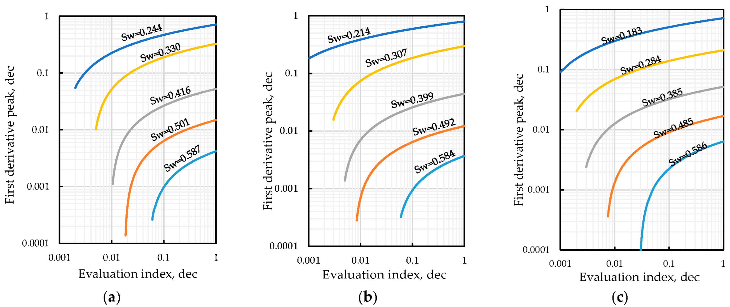
2.3. Classification Chart of DSCs

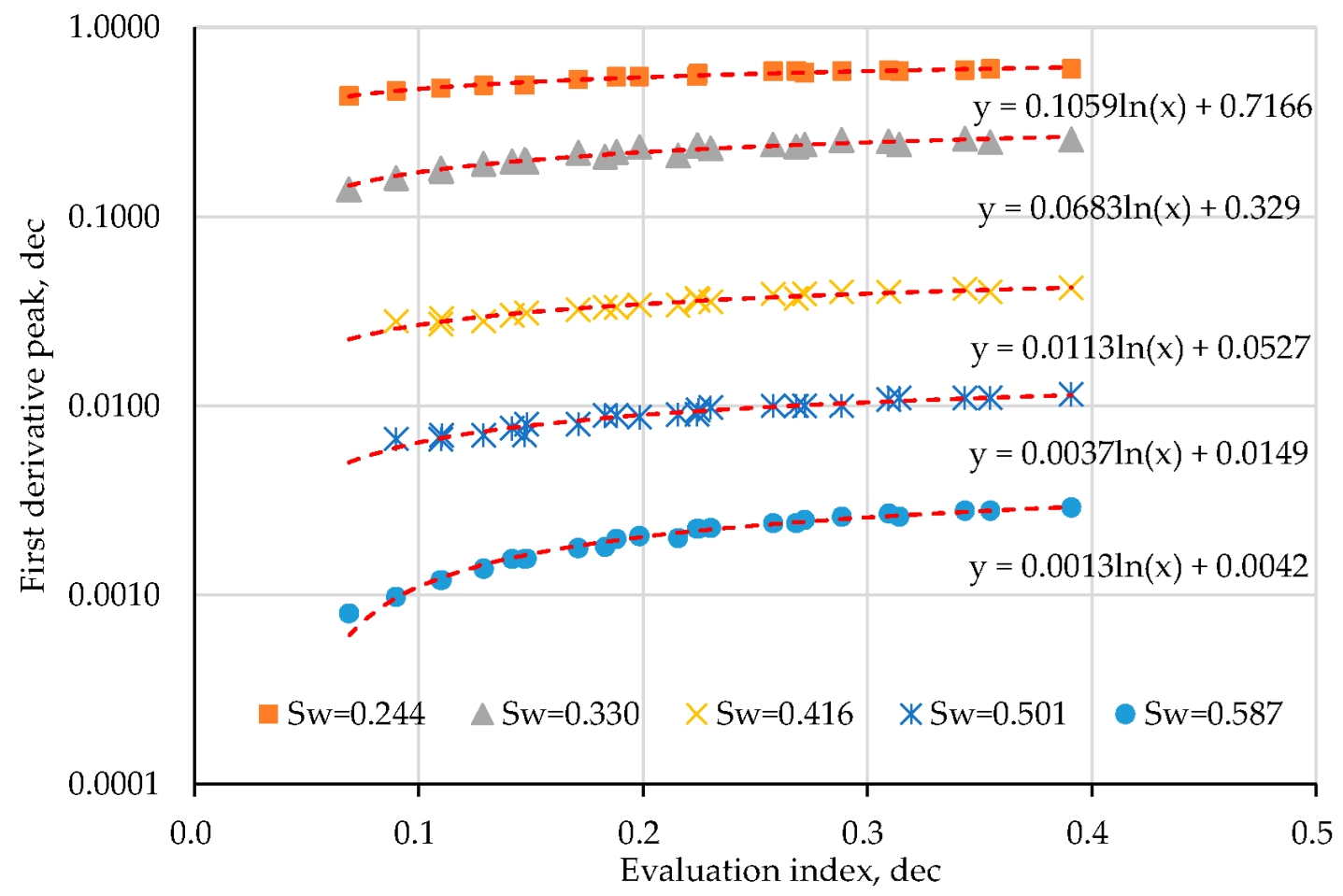
2.3.1. Method for Establishing Classification Chart

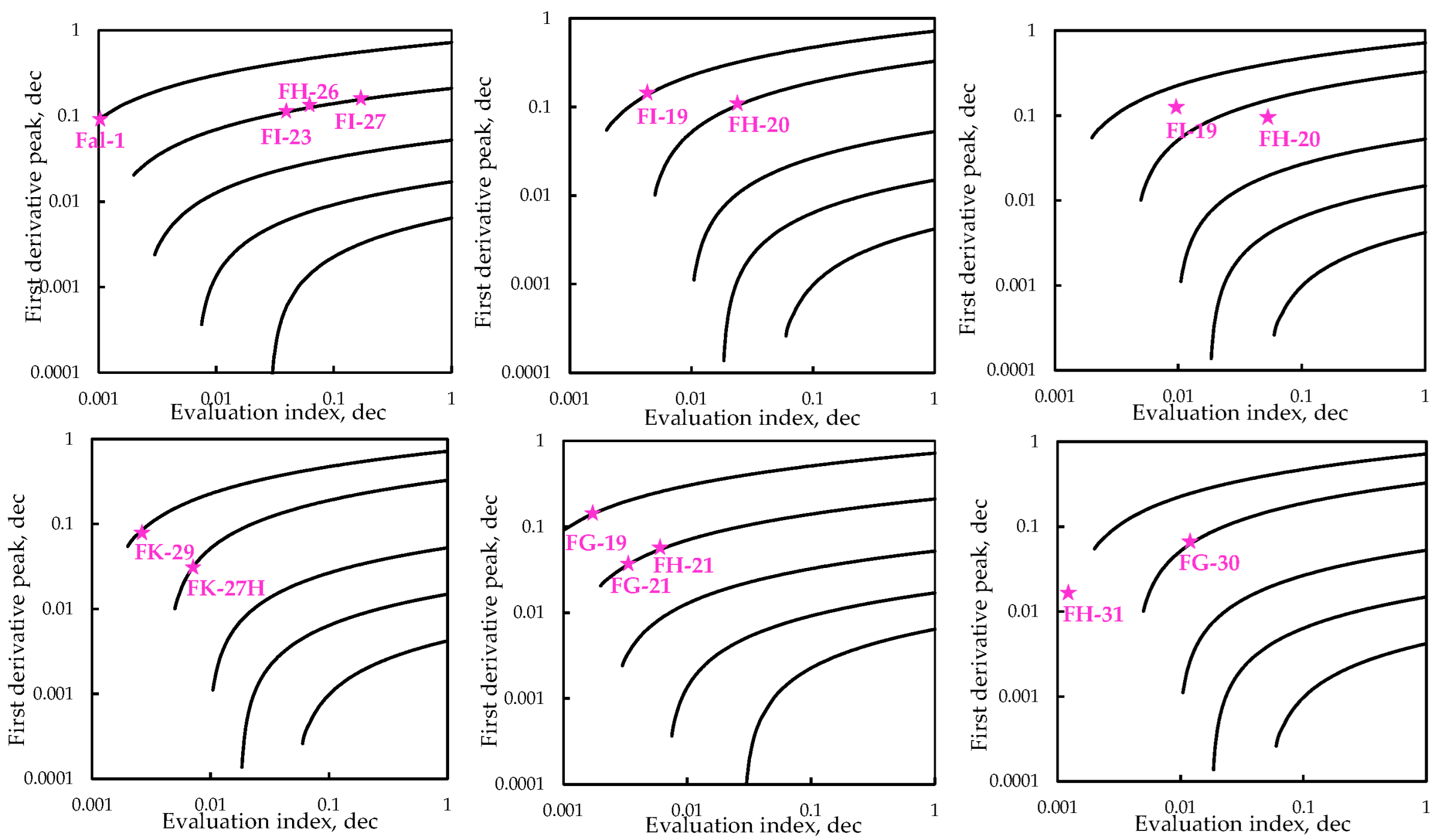
When the DSC is developed in the reservoir, the derivative curve of the water-cut shows double peaks (Figure 1). The dimensionless time and derivative peak corresponding to the first feature point reflect the time and development level of the DSC. Therefore, the first point is selected as the studied object, and the numerical simulation models with different DSCs are constructed according to F_wcr. The β of the first point corresponding to each F_wcr is calculated. Then, the data is regressed. The evaluation formula of DSCs is obtained. According to the formula, the classification chart of DSCs can be drawn. The method for establishing the classification chart of DSCs can be divided into the following seven steps:

Step I—Collect basic data, such as geology, rock, and fluid properties of each layer in the studied area;

Step II—Establish reservoir numerical simulation models with different parameters (α, β, S_wi), and calculate the first peak f′_{w max1} of them;

Step III—Calculate F_wcr according to the α and β set in each DSC model;

Step IV—The f′_{w max1} and F_wcr of each model can be obtained for a certain initial water saturation S_wi. The relationship of f′_{w max1} − F_wcr under the S_wi is obtained through regression data to determine the classification index relationship;

Step V—Establish the relationship between water-cut and water saturation according to the relative permeability curve to determine different water-cut stages;

Step VI—Determine the relationship between F_wcr and f′_{w max1} at different stages according to steps I–III;

Step VII—According to the relationship between F_wcr and f′_{w max1}, the classification chart of DSCs can be drawn.

2.3.2. F_wcr Chart

Based on the oil–water relative permeability and fluid data of each layer in the target reservoir, the water-cut curve with water saturation is produced. At the same time, reservoir numerical simulation models with different permeability, width, and water saturation of DSCs are designed to calculate the water-cut derivative.

(1) Establish the identification index relationship of DSC based on the geological and fluid parameters of layers Y4, Y5, and Y6 in the target reservoir. The average values in the target reservoir parameters are used as the basic parameters of the conceptual model. According to previous studies, the influencing factors of the DSC mainly include permeability of the DSC (K₁), permeability of non-DSCs (K), and initial water saturation (S_wi). Therefore, these parameters are distinguished in each layer. The other parameters are basically consistent. The model parameters are list in

Table 2. Model parameters of layers Y4, Y5, and Y6.

Model Parameters	Values of Y4	Values of Y5	Values of Y6
Model size	30 × 41 × 1	30 × 41 × 1	30 × 41 × 1
K (mD)	1650	2800	3000
w (m)	0.5–4.5	0.5–4.5	0.5–4.5
K1 (mD)	8250–41,250	14,000–70,000	15,000–75,000
Grid size (m)	30 × 10 × 2	30 × 10 × 2	30 × 10 × 2
Swi (dec)	0.244	0.214	0.183
BHP (MPa)	5.0	5.0	5.0
qi (m3/day)	150	150	300

. The curve of water-cut versus water saturation is made from the relative permeability curve. Five groups of water saturation values are selected equally according to the water-cut values, and four numerical models are established, respectively. Four production periods, including low, medium, high, and extra-high production period are simulated. The relationship between the maximum value of the water-cut derivative and the evaluation index is determined. The result of Layer Y4 is shown in Figure 4.

(2) Combined with the relationship between the first derivative peak and evaluation index, the identification chart of DSCs in layers Y4, Y5, and Y6 are established, as shown in Figure 5.

2.3.3. M and N Charts

Based on the oil–water relative permeability and fluid data of each layer in the target reservoir, the water-cut curve with water saturation is produced. At the same time, the reservoir numerical simulation models of DSCs under different α and S_w are designed, and the derivatives of water-cuts are calculated. The relationship between M, N, and α under different S_w values is obtained by regression. According to the relation formula, the charts of M~α and N~α are established, respectively, and the results of Layer Y4 are shown in Figure 6.

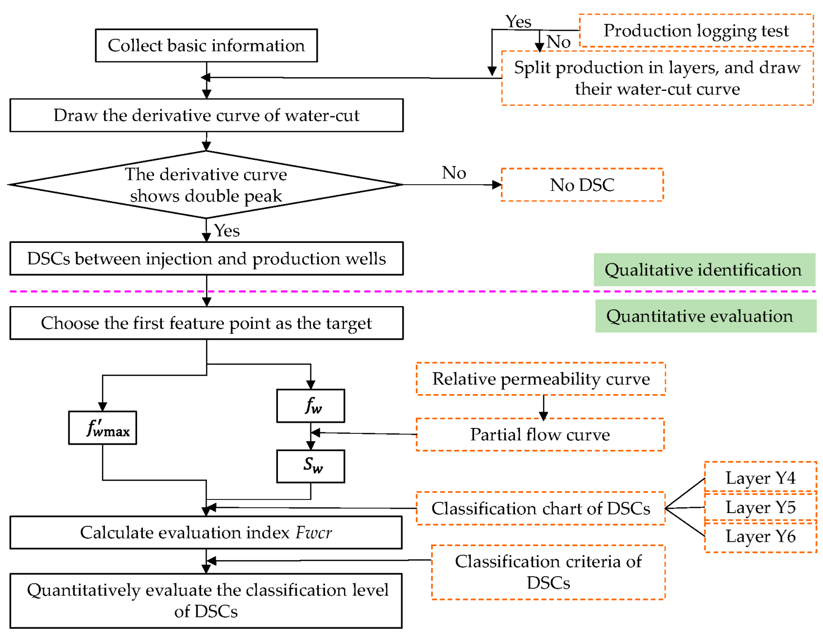
2.4. Evaluation Process of DSCs

The identification method of water-cut derivative is used for the qualitative identification of DSCs, and the static and dynamic data is used for verification. Therefore, the DSC can be identified more accurately. The identification of the DSCs in layered reservoirs is carried out on a plane first and then vertically. The evaluation method of qualitative identification is used first and then quantitative evaluation is employed. The process is shown in Figure 7.

(1)

Qualitative identification of DSCs. Based on the production data of the injection well group, the curve of the water-cut and its derivative with dimensionless time is drawn. If the derivative curve shows double peaks, there is a DSC between the injection and production wells. Otherwise, there is no DSC.

(2)

Identification of DSC among layers. If the DSC exists in the reservoir between injection and production wells, the DSCs among layers can be qualitatively judged and evaluated. It can be carried out in the following two steps:

Step I—Qualitative evaluation of the DSCs among layers. If the injection and production profile data are perfect, the DSCs among layers can be determined directly. If they are not available or incomplete, the splitting coefficient of production in each zone can be calculated according to the splitting method of layered reservoirs. It can be sorted by size. The layer with the largest value develops the DSC.

Step II—Quantitatively evaluate the classification degree of DSCs. On the premise that the reservoir between injection and production well has a DSC and its layer location, the derivative curve of the water-cut can be drawn. The first peak of the water-cut derivative and the water-cut can be obtained. By querying the established F_wcr chart (Figure 5) and classification criteria (Table 1), the evaluation index F_wcr of DSC can be obtained.

3. Application and Discussions

The studied area is located on Melut Basin in South Sudan. The main layers, including Y4, Y5, and Y6, show good petrophysical characteristics (roughly 25% porosity and 1650–3000 mD permeability) and heterogeneous oil (40–300 cp viscosity and 14–20 API) with different aquifer sizes in the layers. There are 13 water injectors in this oilfield. Its production period is about 17 years. Its water-cut is more than 80%. It shows significant difficulties in development because of the heterogeneous formation, oil properties, and natural energy. Some of production wells obviously show the characteristics of a DSC.

Based on the evaluation method of the DSCs in layered reservoirs, the distribution characteristics of the DSCs in the 13 injection groups area are studied. The distribution rules of M and N values corresponding to the first and the second feature points are analyzed (Figure 8 and Figure 9). As shown in the figure, the M and N values can directly reflect the characteristics of the DSC after water flooding.

Taking the production well areas with DSC as the research object, based on the qualitative identification results, the classification chart in each well group is used to evaluate the development degree of DSCs. The evaluation results of some production wells are shown in Figure 10.

According to Figure 10, the F_wcr of the DSCs can be obtained. The development degree of the DSCs can be classified according to the established classification criteria. The evaluation results of some injection groups are shown in

Table 3. Evaluation results of some injection groups.

Injection Group	Production Wells	Layers with DSC	Fwcr	Degree
FI-25	FI-23	Y6	0.0325	Medium
	FH-26	Y6	0.0480	Medium
	FI-27	Y6	0.1928	High
		Y5	0.0589	Medium
	Fal-1	Y6	0.0010	Primary
FI-21	FI-19	Y6	0.0020	Primary
	FH-20	Y6	0.0320	Medium
	FH-23	Y6	0.0568	Medium
	FI-23	Y6	0.0424	Medium
FK-27	FK-27H	Y6	0.0027	Primary
	FK-29	Y6	0.0008	Primary
	FG-19	Y6	0.0011	Primary
FG-20	FH-20	Y6	0.0037	Primary
	FH-21	Y6	0.0081	Primary
FG-31	FG-21	Y6	0.0026	Primary
	FG-30	Y4	0.0203	Medium
	FH-31	Y6	0.0016	Primary

. In the process of oilfield development and production, measures can be taken for injection groups according to the evaluation results. For the area with primary degree of DSCs, the oil recovery can be improved by changing the working schedule of injection-production wells. For medium degree area, the efficiency of water injection and production can be improved by changing the working schedule or the injection-production profile. For high degree area, the contradictions between reservoir layers can be alleviated by adjusting the injection-production profile or the well patterns.

4. Conclusions

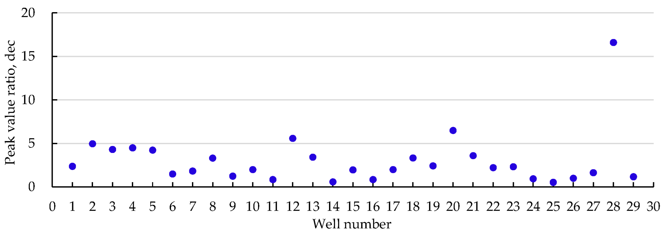
• A method to identify DSCs is established. The derivative curve of the water-cut in the reservoir with the DSC shows double peaks, while the curve without the DSC shows a single peak. After the DSC develops in the reservoir, the derivative curve can be divided into five stages and two feature points. The derivative peak ratio shows obvious regularity;
• A method to evaluate DSCs is established. A new parameter is proposed as the classification index. Combining the characteristic parameters of the derivative curve, the index can be obtained quickly by querying the established F_wcr chart. Furthermore, the development degree of DSC can be evaluated according to the classification criteria.
• The evaluation method of DSCs proposed in this paper is effective in practical applications. The evaluation results show that there are obvious DSCs in some areas. The development degrees are quite different. Corresponding measures are proposed for the area with different development degrees.

References

1. Ding, S.; Jiang, H.; Zhao, Y.; Li, J.; Zhou, D.; Kuang, X. Review on identification of dominant channels in waterflood sandstone reservoirs. Pet. Geol. Eng. 2015, 29, 132–136. [Google Scholar]
2. Zhao, F.; Zhang, G.; Sun, Q.; Xie, T.; Wang, F. Studies on channel plugging in a reservoir by using as a profile control agent in a double-fluid method. Acta Pet. Sin. 1994, 1, 56–65. [Google Scholar]
3. Jiang, H. Early-warning and differentiated adjustment methods for channeling in oil reservoirs at ultra-high water cut stage. J. China Univ. Pet. 2013, 37, 114–119. [Google Scholar]
4. Zeng, L.; Liu, B.; Liu, Y.; Zhang, Y. Study on the influence of dominant channel on water flooding development effect. J. Jianghan Pet. Inst. 2004, 26, 126–127. [Google Scholar]
5. Meng, F.; Sun, T.; Zhu, Y.; Fen, Q. A study on the method to identify large pore paths using conventional well logging data in sandstone reservoirs. Period. Ocean. Univ. China 2007, 37, 463–468. [Google Scholar]
6. Liu, S.; Liang, J. Discussion on the method of identifying invalid injection-production water circulation channel by welltest technology. Welltesting 2004, 13, 27–30. [Google Scholar]
7. Deng, X.; Zhang, X.; Zhu, J.; An, Y. Pattern of preferential reservoir water flow passage and discriminator analysis. Oil Drill. Prod. Technol. 2014, 36, 69–74. [Google Scholar]
8. Wu, S.; Li, Z. The study on identifying macropore path technology. Xinjiang Pet. Sci. Technol. 2010, 20, 27–29. [Google Scholar]
9. Chan, K. Water Control Diagnostic Plots; Society of Petroleum Engineers: Dallas, TX, USA, 1995. [Google Scholar]
10. Yortsos, Y.C.; Choi, Y.; Yang, Z.; Shah, P.C. Analysis and interpretation of water/oil ratio in waterfloods. SPE J. 1999, 4, 413–424. [Google Scholar] [CrossRef]
11. Wang, X.; Xia, Z.; Zhang, H.; Liu, X.; Li, X.; Zhang, L. Study on identification of large orifice with water injection profile logging data. Welltest Technol. 2002, 2, 162–164. [Google Scholar]
12. Shi, L. The application of the micro material inter-well tracing technology in recognizing high capacity channels in oil layer. Pet. Geol. Oilfield Dev. Daqing 2007, 26, 130–132. [Google Scholar]
13. Izgec, B.; Kabir, S. Identification and characterization of high-Conductive layers in waterfloods. SPE Reserv. Eval. Eng. 2011, 14, 113–119. [Google Scholar] [CrossRef]
14. Oftedal, A.; Davies, J.; Kalia, N.; Van Dongen, H. Interwell Communication as a Means to Detect a Thief Zone Using DTS in a Danish Offshore Well; Offshore Technology Conference: Houston, TX, USA, 2013. [Google Scholar]
15. Hao, J. Qualitative identification of prevailing channel by dimensionless pressure index. Spec. Oil Gas Reserv. 2014, 21, 123–125. [Google Scholar]
16. Huang, Y.; Lei, X.; Zhang, Q.; Li, S. Identification technology and application of dominant seepage channel in complex fault block oilfield. Neijiang Technol. 2015, 36, 43–44. [Google Scholar]
17. Ding, S.; Jiang, H.; Wang, L.; Liu, G.; Li, N.; Liang, B. Identification and Characterization of High-Permeability Zones in Waterflooding Reservoirs with an Ensemble of Methodologies; Society of Petroleum Engineers: West Java, Indonesia, 2015. [Google Scholar]
18. Alotaibi, S.; Cinar, Y.; Alshehri, D. Analysis of Water/Oil Ratio in Complex Carbonate Reservoirs under Water-Flood; Society of Petroleum Engineers: Manama, Bahrain, 2019. [Google Scholar]
19. Gu, W. New Method of Water Channeling Identification in Unconsolidated Sandstone Reservoir; Society of Petroleum Engineers: West Java, Indonesia, 2019. [Google Scholar]
20. Lu, C.; Jiang, H.; You, C.; Wang, F.; Xu, F.; Li, J. Determination the levels of thief zones based on machine learning. In Proceedings of the International Petroleum Technology Conference, Virtual, 16 March 2021. [Google Scholar]
21. Ma, R.; Zhao, Z.; Li, Y.; Zou, C.; Hu, D.; Chen, Y.; Zhang, L. A Novel Correction Method for Pressure Transient Analysis Results of Horizontal Wells in Stratified Carbonate Reservoir with High Permeability Zone; Society of Petroleum Engineers: Houston, TX, USA, 2022. [Google Scholar]
22. Fu, L.; Zhao, L.; Chen, S.; Xu, A.; Ni, J.; Li, X. A prediction method for development indexes of waterflooding reservoirs based on modified capacitance–resistance models. Energies 2022, 15, 6768. [Google Scholar] [CrossRef]
23. Kausalysh, N.; Harun, A.R.; Mohd, F.; Rizal, B. Managing Accelerated Water Breakthrough in High Permeability Contrast Waterflood Reservoirs, and Achieving Production Conformance through Injection Redistribution Strategy; Society of Petroleum Engineers: Dubai, UAE, 2022. [Google Scholar]
24. Qi, Q.; Iraj, E. Modeling of Injection-Induced Particle Movement Leading to the Development of Thief Zones; Society of Petroleum Engineers: Houston, TX, USA, 2017. [Google Scholar]
25. Albertoni, A.; Lake, L.W. Inferring inter-well connectivity only from well-rate fluctuations in waterfloods. SPE Reserv. Eval. Eng. 2003, 6, 6–16. [Google Scholar] [CrossRef]
26. Weber, D. The Use of Capacitance-Resistance Models to Optimize Injection Allocation and Well Location in Water Floods. Ph.D. Thesis, University of Texas, Austin, TX, USA, 2009. [Google Scholar]
27. Parekh, B.; Kabir, C.S. A case study of improved understanding of reservoir connectivity in an evolving waterflood with surveillance data. J. Pet. Sci. Eng. 2013, 102, 1–9. [Google Scholar] [CrossRef]
28. Zhang, Z.; Li, H.; Zhang, D. Water flooding performance prediction by multi-layer capacitance-resistive models combined with the ensemble Kalman filter. J. Pet. Sci. Eng. 2015, 127, 1–19. [Google Scholar] [CrossRef]
29. Wang, Q.; Liu, X.; Meng, L.; Jiang, R.; Fan, H. The numerical simulation study of the oil-water seepage behavior dependent on the polymer concentration in polymer flooding. Energies 2020, 13, 5125. [Google Scholar] [CrossRef]
30. Negash, B.M.; Yaw, A.D. Artificial neural network based production forecasting for a hydrocarbon reservoir under water injection. Pet. Explor. Dev. 2020, 47, 357–365. [Google Scholar] [CrossRef]
Figure 1. (a) Curve features of water-cut derivative in the reservoir with DSC and non-DSC. (b) Saturation distribution of injected water in the reservoir with DSC.
Energies 15 08833 g001
Figure 2. (a) Relationship between derivative peak ratio (M) and permeability ratio (α). (b) Relationship between M and width ratio (β). (c) Relationship between M and initial water saturation (Swi).
Energies 15 08833 g002
Figure 3. (a) Relationship between time ratio (N) and α. (b) Relationship between N and β. (c) Relationship between N and Swi.
Energies 15 08833 g003
Figure 4. Relation curves between first derivative peak (f′w max1) and evaluation index (Fwcr) in Layer Y4 with different water saturations.
Energies 15 08833 g004
Figure 5. (a) The evaluation index (Fwcr) chart of DSCs in Layer Y4. (b) The Fwcr chart of DSCs in Layer Y5. (c) The Fwcr chart of DSCs in Layer Y6.
Energies 15 08833 g005
Figure 6. (a) Chart of derivative peak ratio (M)~permeability ratio (α) in Layer Y4. (b) Chart of time ratio (N)~permeability ratio (α) in Layer Y4.
Energies 15 08833 g006
Figure 7. The evaluation process chart of DSCs.
Energies 15 08833 g007
Figure 8. M values in the production well area with DSC.
Energies 15 08833 g008
Figure 9. N values in the production well area with DSC.
Energies 15 08833 g009
Figure 10. Classification chart of DSCs in some areas of production wells.
Energies 15 08833 g010