
Evaluation of Photovoltaic Consumption Potential of Residential Temperature-Control Load Based on ANP-Fuzzy and Research on Optimal Incentive Strategy

Abstract
:1. Introduction
2. ANP-Fuzzy Prediction Model
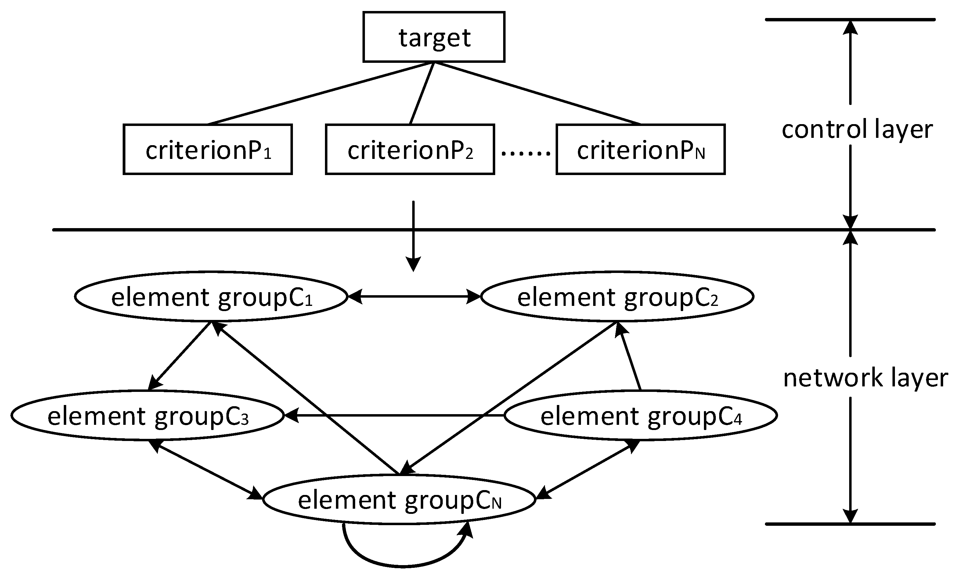
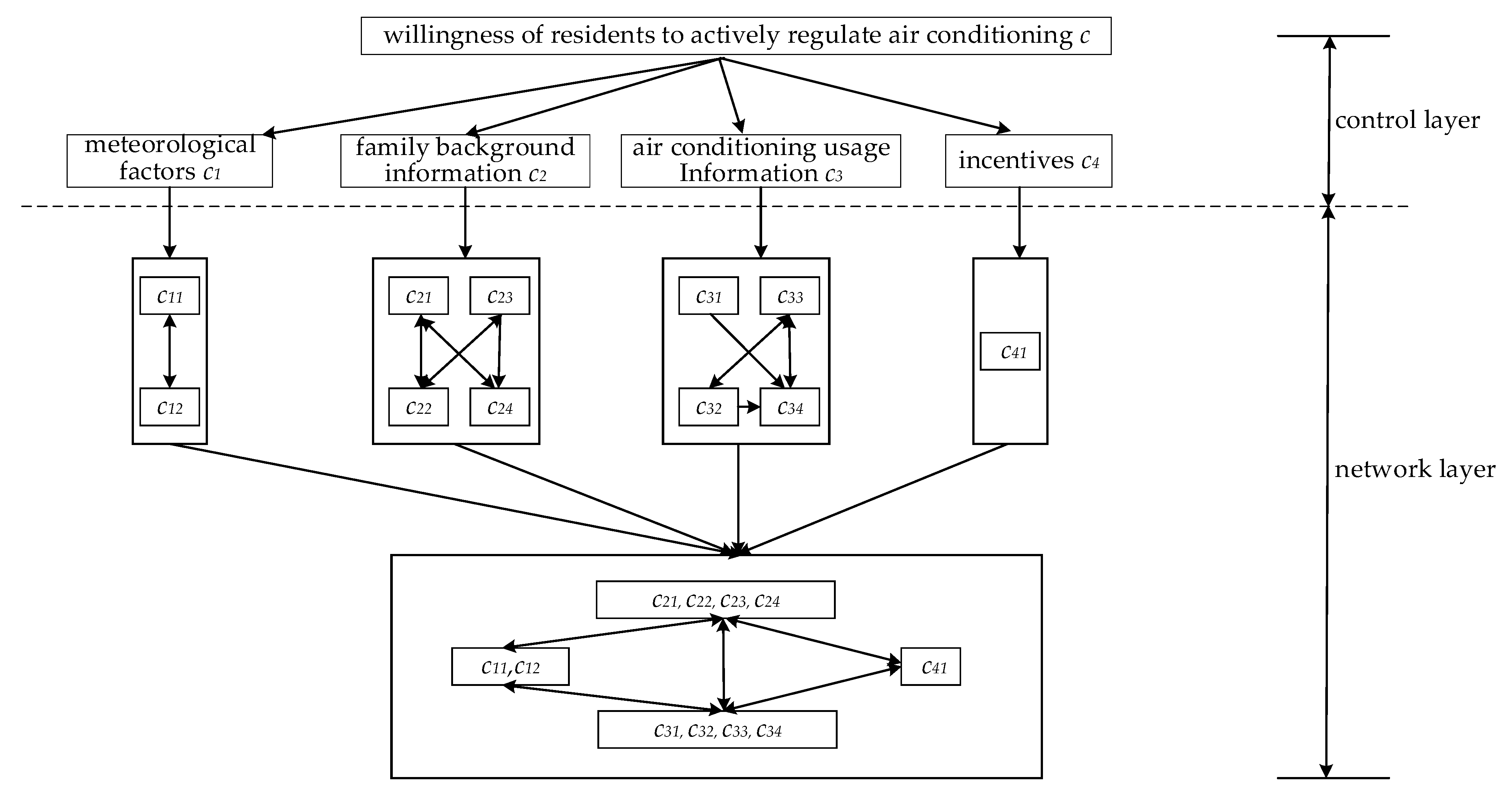
2.1. Establishment of Evaluation Index System Based on ANP
2.2. ANP-Fuzzy Implementation Steps
- Establish the 2-layer ANP network model
- 2.
- Identify element importance and generate comparison judgment matrix
- 3.
- Calculate weight vector of each element group
- 4.
- Generate weighted supermatrix
- 5.
- Perform supermatrix stability processing
- 6.
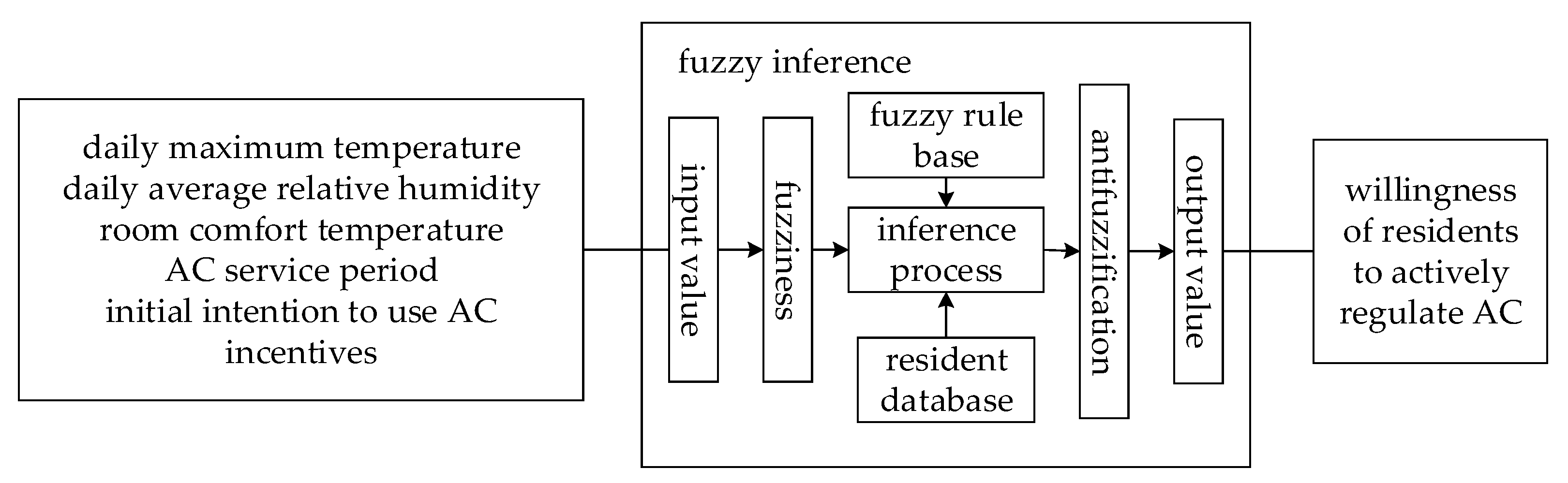
- Establish fuzzy inference model and perform fuzzy processing
- 7.
- Construct membership function
- 8.
- Formulate fuzzy rules
- 9.
- Output prediction results and perform model correction
3. Day-Ahead Dispatch Based on Price-Incentive Load Potential Assessment
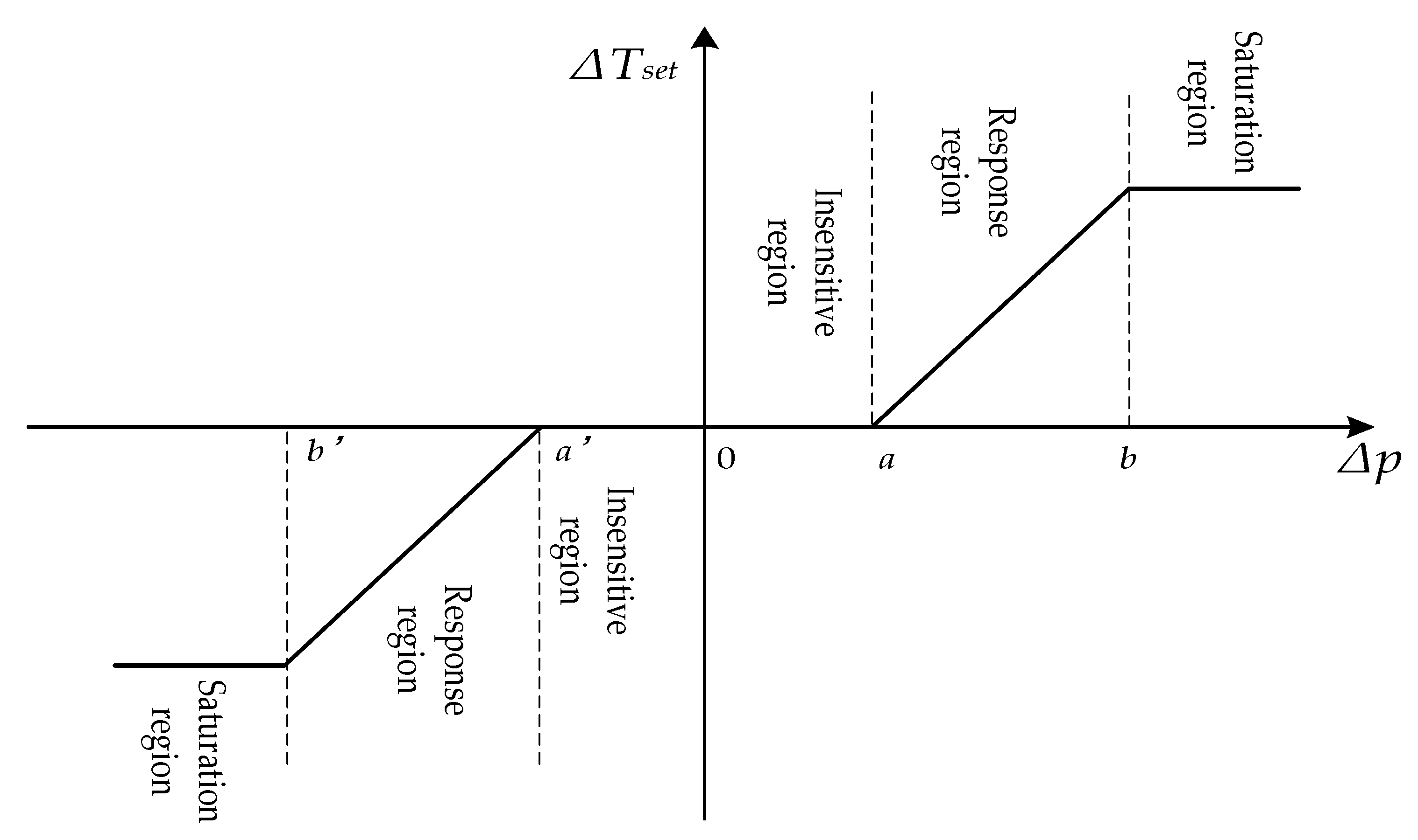
3.1. Price-Based Residential Load Demand Response
3.2. User Comfort Price Compensation Model
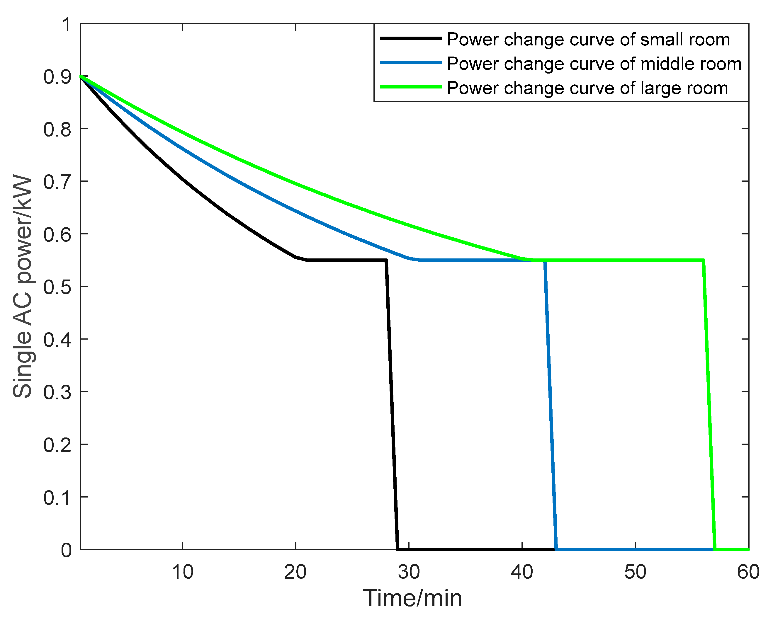
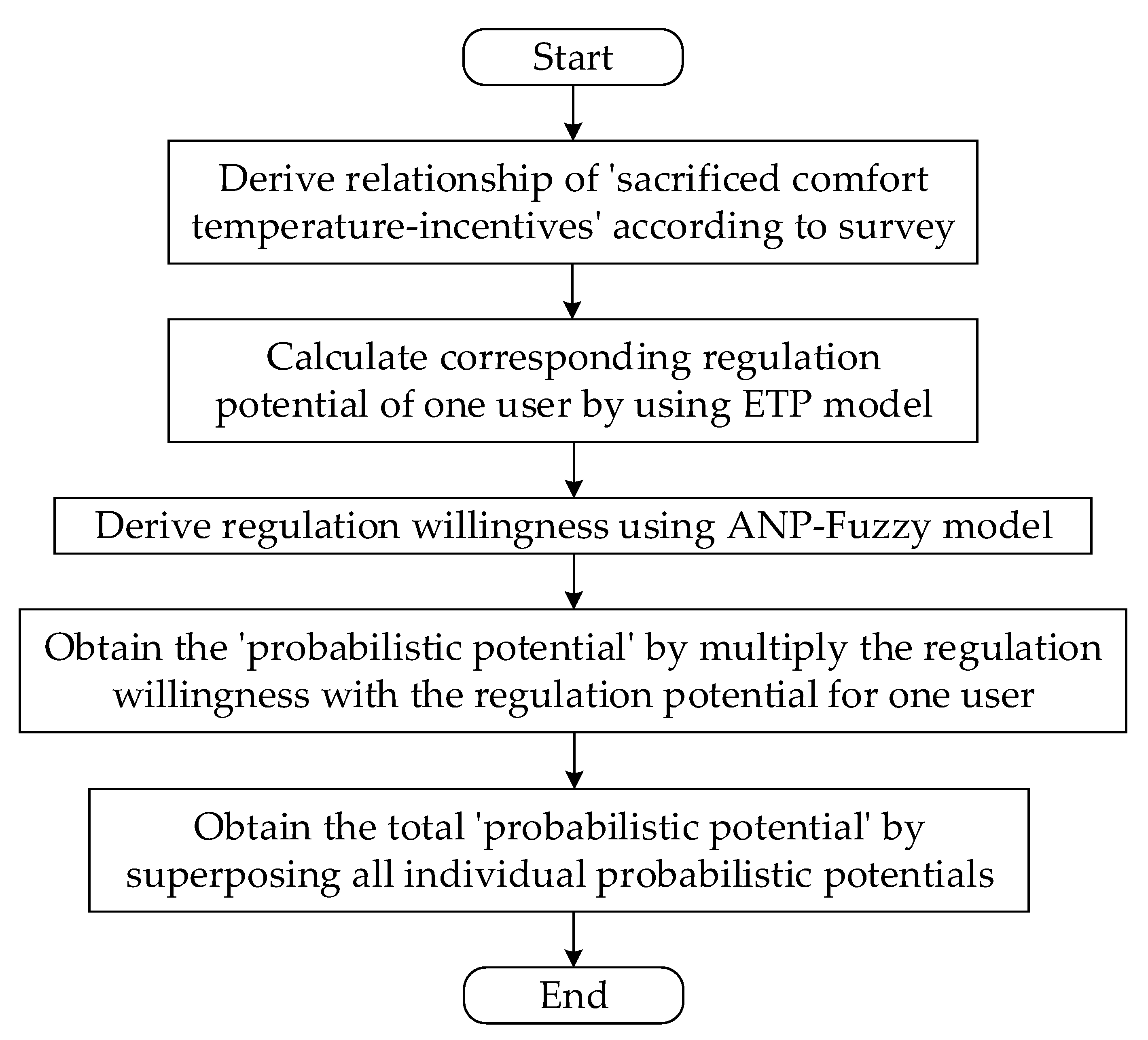
3.3. Prediction of Adjustable Power Potential of Residential AC
3.4. Day Ahead Dispatching Model of Power System
4. Case Analysis
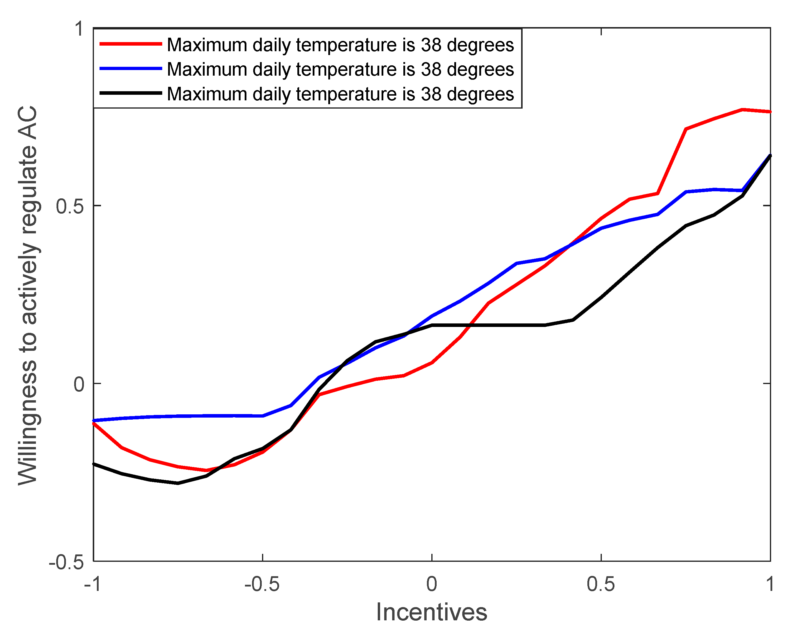
4.1. Using ANP-Fuzzy Model to Predict Residents’ Willingness to Actively Regulate AC
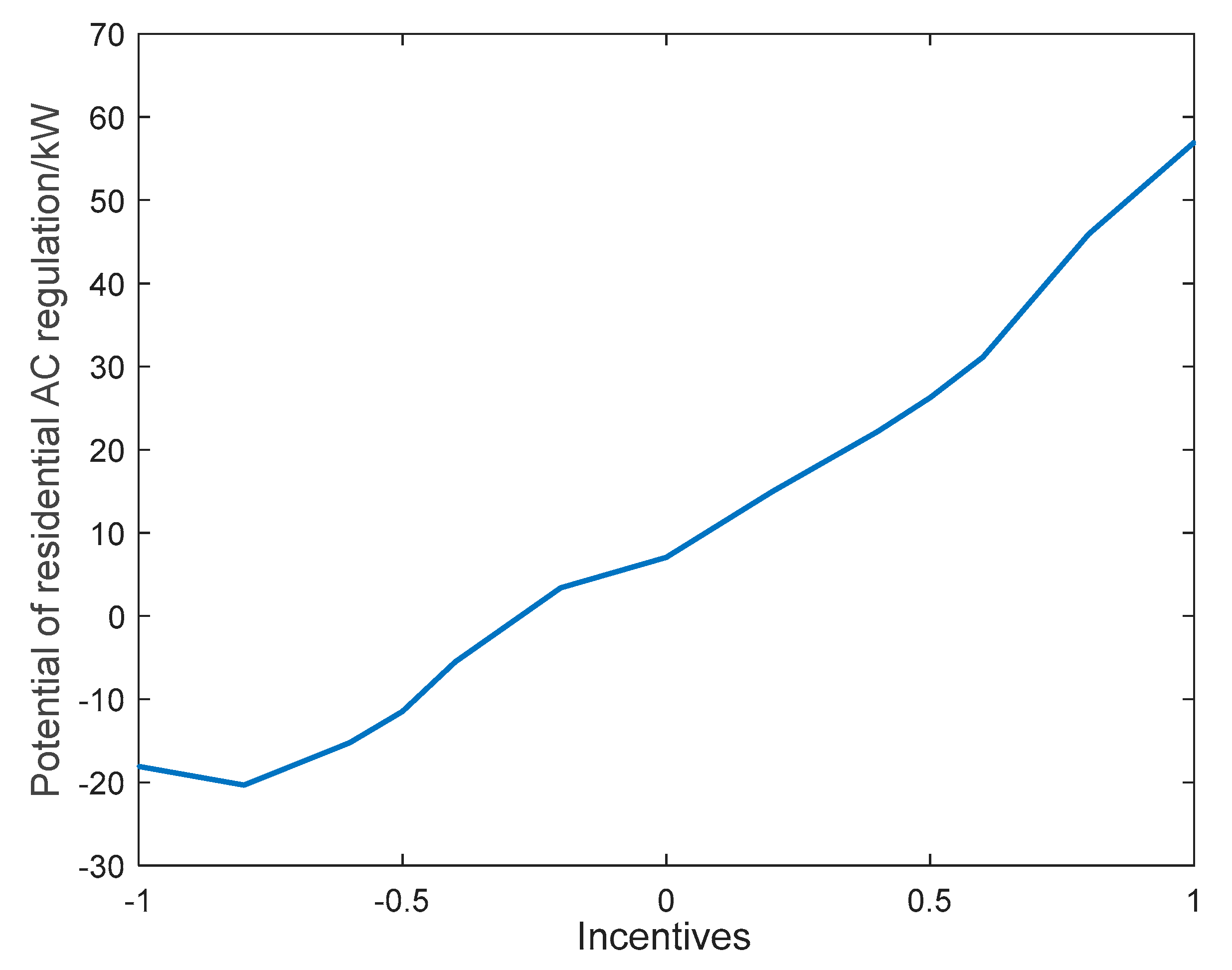
4.2. Prediction of Adjustable Power Potential of Residential ACs
4.3. Day Ahead Dispatching Model of Power System
4.4. Discussion
5. Conclusions
Author Contributions
Funding
Data Availability Statement
Conflicts of Interest
References
- Pathiravasam, C.; Venayagamoorthy, G.K. Distributed Demand Response Management for a Virtually Connected Community with Solar Power. IEEE Access 2022, 10, 8350–8362. [Google Scholar] [CrossRef]
- Xu, Q.; Ding, y.; Yan, Q. Research on Evaluation of Scheduling Potentials and Values on Large Consumers. Proc. CSEE 2017, 37, 6791–6800. [Google Scholar]
- Yang, Y.; Wang, T.; Chen, X. Multi-power level control strategy of an electric heating cluster considering new energy consumption. Power Syst. Prot. Control 2022, 50, 20–30. [Google Scholar]
- Qiu, G.; He, C.; Luo, Z. Economic dispatch of Stackelberg game in distribution network considering new energy consumption and uncertainty of demand response. Electr. Power Autom. Equip. 2021, 41, 66–72. [Google Scholar]
- Wang, J.; Chen, X.; Xie, J.; Xu, S.; Yu, K.; Gan, L. Control Strategies of Large-scale Residential AC Loads Participating in Demand Response Programs. CSEE J. Power Energy Syst. 2022, 8, 880–893. [Google Scholar]
- Montrose, R.S.; Gardner, J.F.; Satici, A.C. Centralized and Decentralized Optimal Control of Variable Speed Heat Pumps. Energies 2021, 14, 4012. [Google Scholar] [CrossRef]
- Xia, S.; Ding, Z.; Du, T.; Zhang, D.; Shahidehpour, M.; Ding, T. Multitime Scale Coordinated Scheduling for the Combined System of Wind Power, Photovoltaic, Thermal Generator, Hydro Pumped Storage, and Batteries. IEEE Trans. Ind. Appl. 2020, 56, 2227–2237. [Google Scholar] [CrossRef]
- Zhang, J.; Jiang, F.; Wu, H. Dual market bidding strategy of load aggregator based on CVaR. Electr. Power Autom. Equip. 2020, 40, 153–158. [Google Scholar]
- Iftikhar, H.; Sarquis, E.; Branco, P.J.C. Why Can Simple Operation and Maintenance (O&M) Practices in Large-Scale Grid-Connected PV Power Plants Play a Key Role in Improving Its Energy Output? Energies 2021, 14, 3798. [Google Scholar]
- Ma, X.; Wang, G.; Zhu, S. Coordinated Day-Ahead Optimal Dispatch Considering Wind Power Consumption and the Benefits of Power Generation Group. Trans. China Electrotech. Soc. 2021, 36, 579–587. [Google Scholar]
- Yang, X.; Fu, G.; Liu, F. Potential Evaluation and Control Strategy of AC Load Aggregation Response Considering Multiple Factors. Power Syst. Technol. 2022, 46, 699–708. [Google Scholar]
- Zhu, Y.; Wang, J.; Cao, X. Direct control strategy of central air-conditioning load and its schedulable potential evaluation. Electr. Power Autom. Equip. 2018, 38, 227–234. [Google Scholar]
- Sun, Y.; Liu, D.; Cui, X. Equal gradient iterative learning incentive strategy for accurate demand response of resident users. Power Syst. Technol. 2019, 43, 3597–3605. [Google Scholar]
- Li, W.; Wang, Q.; Zhang, H. Research on Counter measures to solve the problem of abandoned wind power: Based on the theory of price regulation mechanism and case analysis. Price Theory Pract. 2013, 2, 53–54. [Google Scholar]
- Li, W.; Yang, Q.; Zhang, H. Incentive mechanism research on accommodation of wind power in regional electricity market based on cooperative game. Renew. Energy Resour. 2014, 32, 475–480. [Google Scholar]
- Zhou, J.; Su, X.; Qian, H. Risk Assessment on Offshore Photovoltaic Power Generation Projects in China Using D Numbers and ANP. IEEE Access 2020, 8, 144704–144717. [Google Scholar] [CrossRef]
- Lan, L.T.H.; Tuan, T.M.; Ngan, T.T.; Giang, N.L.; Ngoc, V.T.N.; Van Hai, P. A New Complex Fuzzy Inference System with Fuzzy Knowledge Graph and Extensions in Decision Making. IEEE Access 2020, 8, 164899–164921. [Google Scholar]
- Yang, M.; Wang, Y.; Gao, S.; Zhang, Q.; Li, Z.; Wang, D. A bidding model for virtual power plants to participate in demand response in the new power market environment. In Proceedings of the 2021 International Conference on Power System Technology (POWERCON), Haikou, China, 8–9 December 2021. [Google Scholar]
- Zheng, S. Incentive-Based Integrated Demand Response for Multiple Energy Carriers Considering Behavioral Coupling Effect of Consumers. IEEE Trans. Smart Grid 2020, 11, 3231–3245. [Google Scholar] [CrossRef]
- Jia, Q.; Chen, S.; Yan, Z.; Li, Y. Optimal Incentive Strategy in Cloud-Edge Integrated Demand Response Framework for Residential AC Loads. IEEE Trans. Cloud Comput. 2022, 10, 31–42. [Google Scholar] [CrossRef]
- Huo, M.; Chen, L.; Niu, Z. AC Load Demand Response Strategy for Distributed Photovoltaic Power Accommodation. Power Energy 2021, 42, 313–319. [Google Scholar]
- Yang, Z.; Ding, X.; Lu, X. Inverter air conditioner load modeling and operational control for demand response. Power Syst. Prot. Control 2021, 49, 132–140. [Google Scholar]
- Wu, C.; Shen, H.; Wang, Z. Data-driven Online Identification Method for Parameters of Inverter Air-conditioning Load Model. Autom. Electr. Power Syst. 2022, 46, 120–129. [Google Scholar]


| Target | Factor Set (4 Grade-1 Indicators) | Sub-Element Set (11 Grade-2 Indicators) |
|---|---|---|
| Willingness of residents to actively regulate AC c | meteorological factors c1 | daily maximum temperature c11 |
| average daily relative humidity c12 | ||
| family background information c2 | annual household income c21 | |
| age distribution of family members c22 | ||
| room comfort temperature c23 | ||
| house size c24 | ||
| AC usage information c3 | number of air conditioners c31 | |
| AC installation location c32 | ||
| AC usage time c33 | ||
| initial willingness to use ACs c34 | ||
| incentives c4 | price incentive c41 |
| Room Type | C/((kW·h)/°C−1) | R/(°C·kW−1) |
|---|---|---|
| Small room | 0.147 | 10.6 |
| Medium room | 0.218 | 10.2 |
| Large room | 0.286 | 9.7 |
| Indicators | Local Weight | Global Stability Weight |
|---|---|---|
| daily maximum temperature c11 | 0.5455 | 0.2385 |
| average daily relative humidity c12 | 0.4545 | 0.1987 |
| annual household income c21 | 0.1611 | 0.0392 |
| age distribution of family members c22 | 0.1607 | 0.0391 |
| room comfort temperature c23 | 0.6017 | 0.1466 |
| room size c24 | 0.0765 | 0.0186 |
| number of ACs c31 | 0.0301 | 0.0049 |
| AC installation location c32 | 0.0537 | 0.0089 |
| AC usage time period c33 | 0.4971 | 0.0827 |
| initial willingness to use ACs c34 | 0.4193 | 0.0697 |
| incentive price c41 | 1.0000 | 0.0621 |
| Inputs | Values |
|---|---|
| daily maximum temperature c11 | 28, 34 and 38 °C |
| average daily relative humidity c12 | 65% |
| room comfort temperature c23 | 24 °C |
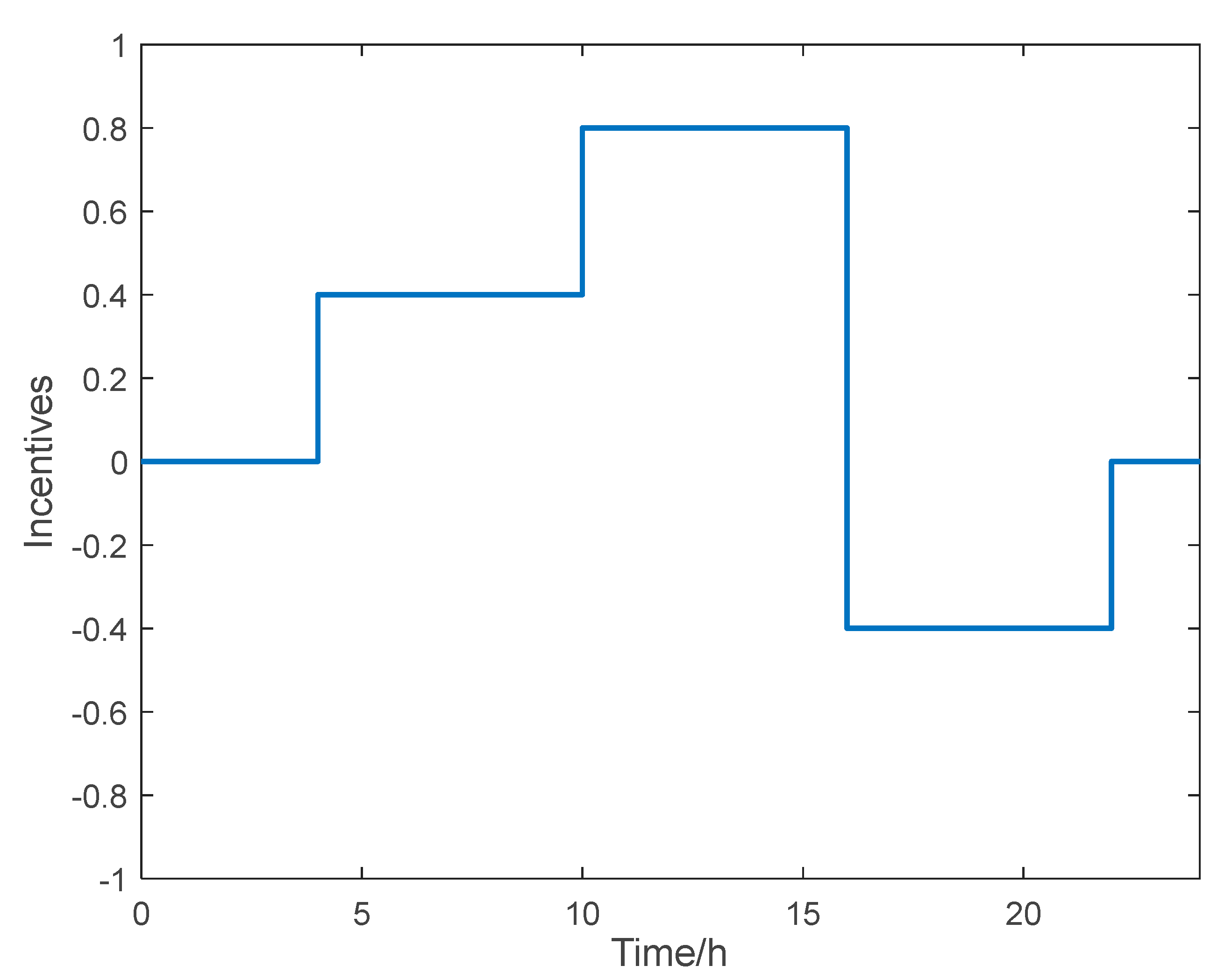
| AC usage time period c33 | 4–10, 10–16, 16–22, 22–4 |
| initial willingness to use ACs c34 | 50% |
| incentive price c41 | −1~1(corresponding to −0.5~0.5 RMB yuan) |
Publisher’s Note: MDPI stays neutral with regard to jurisdictional claims in published maps and institutional affiliations. |
© 2022 by the authors. Licensee MDPI, Basel, Switzerland. This article is an open access article distributed under the terms and conditions of the Creative Commons Attribution (CC BY) license (https://creativecommons.org/licenses/by/4.0/).
Share and Cite
Lu, S.; Li, T.; Yan, X.; Yang, S. Evaluation of Photovoltaic Consumption Potential of Residential Temperature-Control Load Based on ANP-Fuzzy and Research on Optimal Incentive Strategy. Energies 2022, 15, 8640. https://doi.org/10.3390/en15228640
Lu S, Li T, Yan X, Yang S. Evaluation of Photovoltaic Consumption Potential of Residential Temperature-Control Load Based on ANP-Fuzzy and Research on Optimal Incentive Strategy. Energies. 2022; 15(22):8640. https://doi.org/10.3390/en15228640
Chicago/Turabian StyleLu, Siyue, Teng Li, Xuefeng Yan, and Shaobing Yang. 2022. "Evaluation of Photovoltaic Consumption Potential of Residential Temperature-Control Load Based on ANP-Fuzzy and Research on Optimal Incentive Strategy" Energies 15, no. 22: 8640. https://doi.org/10.3390/en15228640
APA StyleLu, S., Li, T., Yan, X., & Yang, S. (2022). Evaluation of Photovoltaic Consumption Potential of Residential Temperature-Control Load Based on ANP-Fuzzy and Research on Optimal Incentive Strategy. Energies, 15(22), 8640. https://doi.org/10.3390/en15228640