Economic Assessment of Demand Response Using Coupled National and Regional Optimisation Models

Abstract

In this work, we investigate the economic viability of demand response (DR) as a balancing option for variable renewable energies, such as wind and solar. Our assessment is based on a highly resolved national energy system model for Germany coupled with a regional DR optimisation model. First, this allows us to determine the spatially resolved flexibility demand, e.g., for avoiding transmission grid congestion. Second, a high number of DR technologies from the residential, commercial and industrial sector, as well as sector coupling, can be considered to cover the regional flexibility demand. Our analysis is based on a scenario for 2035 with a $66\%$ share of renewable energy sources in the power generation. The results show that the largest DR capacity is being installed in the west of Germany, an area with a high density of population and industry. All DR units have an aggregated capacity below 100 MW per transmission grid node. For the economic assessment, we further differentiate between two cases. In the first case with full DR cost consideration, the optimisation selects only large-scale technologies with low specific investment costs. The second case assumes that the required communication components are already installed. Here, we consider only variable costs and disregard the investment costs. As a result, several small-scale DR technologies are used, such as e-mobility. We publish the developed methodology as an open-source model, which allows reuse for other scientific purposes.

1. Introduction

In order to reduce CO${}_2$ emissions and mitigate climate change, governments worldwide set goals for renewable energy development [1,2]. As part of the “Fit for 55” package, aiming at a greenhouse gas emissions reduction of $55\%$ by 2030, the European Commission recently proposed to increase the overall renewables target for 2030 from 32 to $40\%$ [3]. However, an increasing weather-dependent feed-in power by variable renewable energies (VRE), such as wind power and photovoltaics (PV), leads to a higher demand for power system balancing [4]. Such balancing requirements can be provided, e.g., by energy storages [5], dispatchable conventional generators [6], demand response (DR) [7] or electricity grid expansion [8]. Currently, DR plays a minor role [9] but may gain importance in future, as it includes the increasing number of stakeholders actively participating in energy demand and supply at a regional level (e.g., distributed small-scale technologies) [10]. DR can be further distinguished, as follows [11]: Load shedding is associated with loads being reduced that cannot be compensated for at another time [12]. Load shifting applies to loads being shifted from one time point to another, e.g., from a period with a low VRE feed-in tariff to a period with a high VRE feed-in tariff [13]. As only load shifting can contribute to avoid VRE curtailment in times where the feed-in power exceeds demand or grid capacity, we disregard load shedding in this work.

Amongst others, there are two main categories of studies in the literature considering the economic assessment of DR. The first type of studies assess DR from an energy system’s perspective taking, e.g., a whole country or even multiple countries into account. Kies et al. [14] investigated the potential of DR to balance a fully renewable European power system, using a power-flow model with one node per country. The analysis yielded that DR reduced the need for backup energy by up to one third and the optimal mix of wind energy and DR substantially increased the economic performance of PV. Misconel et al. [10] determined the potential role of DR in Europe and its impact on the optimal combination of flexibility options in a decentralised vs. centralised $100\%$ renewable scenario framework. The model results showed a higher reduction of total system costs and CO${}_2$ emissions per activated DR unit in the decentralised scenario compared to the centralised scenario. Kirkerud et al. [15] examined the economic potential of DR in the northern European region and analysed the power market impacts. The results showed that space heating and water heating provided the highest shares of loads shifted. DR contributed to peak shaving of up to $18.6\%$ of total peak load. Gils [16] assessed the economic DR potential in Germany using a power-flow model with six nodes, each representing one region of the country. In the case study with a VRE share of $70\%$, DR substituted more than 5 GW of power plant capacity and reduced power supply costs by several hundreds of millions of euros.

The second type of studies investigate DR based on specific demonstration projects. According to Gangale et al. [17], more than 300 research projects have been carried out in Europe that include DR demonstration. As part of the enera project [18], a resistive heating unit was installed in a paper factory. The facility could increase its load in times of high wind generation and convert excess feed-in power to process heat, providing a load increase potential of 4.6 MWh. The economic viability was hampered by the high share of taxes, levies and grid charges at the power prices. During the NEW 4.0 project [19], dynamic electricity tariffs were offered to 1000 private households in the city of Norderstedt in Germany. Incentivised by price reductions of more than $50\%$, demand was shifted to times with high VRE feed-in tariff. On average, an amount of 22 kWh was shifted per customer and month, which corresponded to approximately $10\%$ of the monthly electricity demand. In the project London low carbon [20], the DR potential of electric vehicle charging facilities was investigated. Based on measurement data from 70 residential charging facilities in London, the authors found that by controlled charging, a peak load reduction of $24\%$ could be achieved.

In summary, the first mentioned type of studies that investigated DR from a system’s perspective have in common that due to a higher generalisation the technological detail is lower. Particularly in studies with energy-system optimisation models, as e.g., [14,16], the computation time is a limiting factor. Thus, a trade-off needs to be made between the spatial detail of the modelling, e.g., the number of power grid nodes, the temporal detail, e.g., the number of time steps, and the technological detail, e.g., the number of considered technologies or the number of optimisation variables modelling the behaviour of the technologies. The economic assessment carried out in these kinds of studies is mostly based on a macroeconomic perspective.

In comparison, the second mentioned type of studies that investigate DR based on demonstration projects focus on a delimited geographic region, e.g., a city, or even just one industrial plant. In most cases, there is no extensive optimisation problem to be solved in these studies, instead more technological details are considered. The economic assessment in the latter kind of studies is typically carried out from the perspective of the operator of the DR technologies.

To our knowledge the present work is the first that closes the gap between both kind of studies, which is an important contribution for the following reasons. Generalised national energy system models (first type of studies) require feedback from regional demonstration projects (second type of studies). For example, DR can be found to be beneficial from a simplified macroeconomic assessment [14,16], but may not be economically viable from an operator’s perspective, e.g., in a specific industrial facility [18]. The other way around, a holistic economic assessment of a DR process at a specific location requires input data from national energy system models. For example, time series of the flexibility demand of the total power system are needed as well as information about how much competing DR units are present in the system.

The combination of both approaches is achieved in this work as follows. We include a simplified DR representation in the national energy system model eTraGo (electric transmission grid optimisation) (For more information visit: https://etrago.readthedocs.io/en/latest/index.html, accessed on 27 September 2022) [21] for Germany and couple it with a more detailed, regional DR optimisation. Both are implemented in the newly developed model region4FLEX (region for flexibility) (For more information visit: https://wiki.openmod-initiative.org/wiki/Region4FLEX, accessed on 27 September 2022) [22]. In this manner, the macroeconomic optimisation in eTraGo is combined with an economic assessment from the operator’s perspective in the region4FLEX model using the net present value method [23].

The second novel aspect of the present study is the power grid resolution of the applied energy system model. Frysztacki et al. [24] showed that a higher network resolution revealed more critical bottlenecks in the transmission system. For this reason, a high network resolution also seems a prerequisite for the economic assessment of DR as a measure for avoiding power grid overloading and VRE curtailment. While other DR studies based on energy system models have a comparable low spatial resolution, e.g., six regions (nodes) for Germany [16] or one node per country in Europe [14], we apply an energy system model with 1000 nodes for Germany.

The third novel aspect of the present study is that the impact of technological modelling detail on the economic viability of DR is investigated. In addition to the 19 considered DR technologies from the residential, commercial, industrial, power-to-heat, e-mobility and power-to-gas sector, we further analyse the effect of introducing heat pump size classes.

In particular, this paper examines the following research questions:

• Where are DR units allocated in a high-resolution German power grid model and when are they dispatched?
• What is the average break-even revenue for DR from a generalised system’s perspective and a more detailed regional perspective?
• Which technologies are most economically viable?
• What are the influences on the economic viability of demand response?

The remaining sections of this paper are structured as follows. Section 2 describes the applied methodology and the used input data. Section 3 presents the results for the allocation and dispatch of the DR units, the economic assessment, a sensitivity analysis and a critical appraisal. Section 4 summarises the main conclusions of the study and provides an outlook.

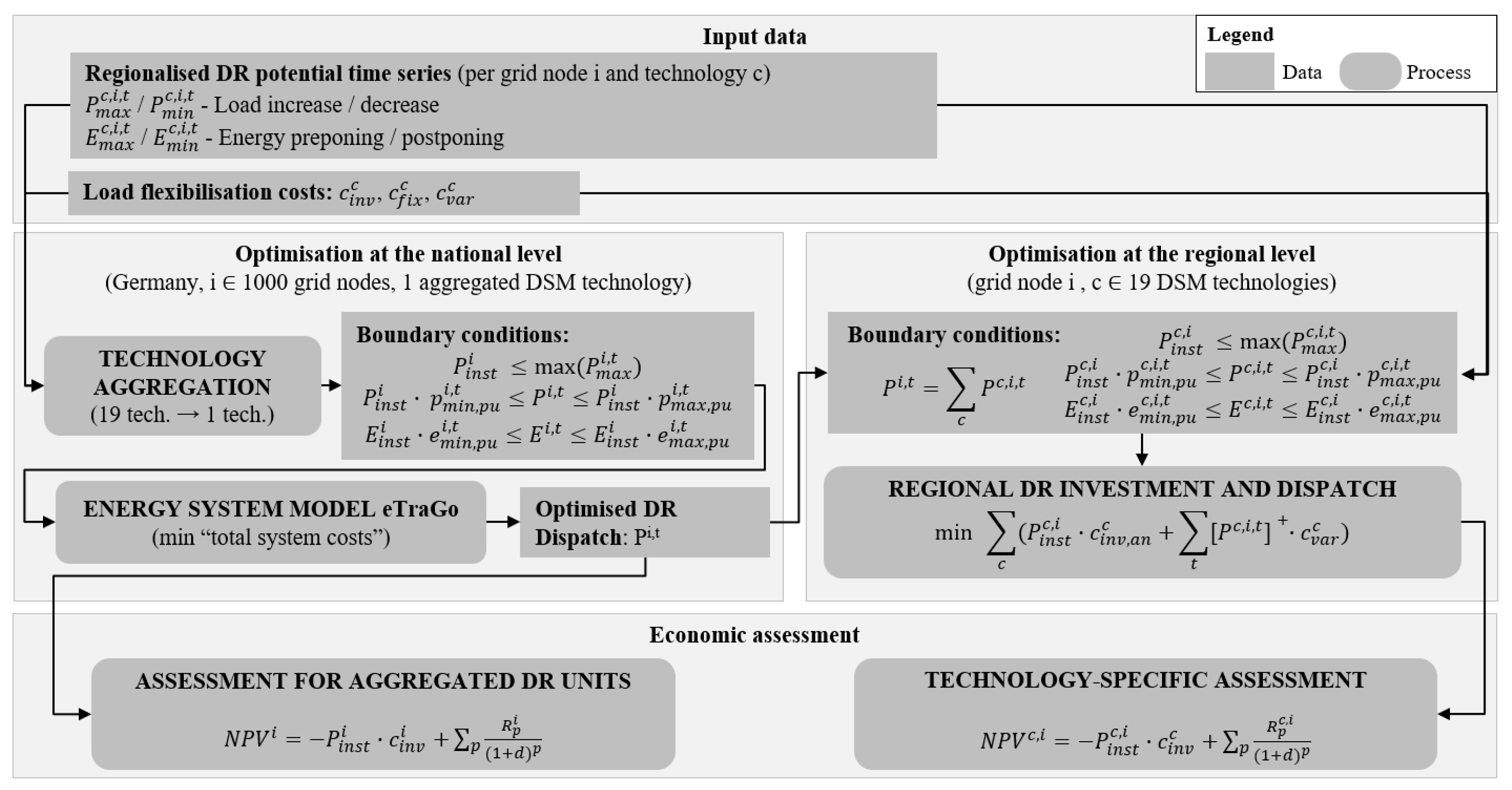
2. Methods and Input Data

The used input data and applied methodology in this work are summarised in Figure 1. The main input data were the regionalised DR potential time series and the load flexibilisation costs, which are further described in Section 2.1. We first used these input data for implementing DR in the optimisation model at the national level (eTraGo), using one aggregated DR unit per transmission grid node (Section 2.2). This allowed us to solve the model with a high spatial resolution of 1000 grid nodes. Among others, the results of the optimisation at the national level were the installed DR capacities per grid node and the time series of the DR dispatch. These data were further used in the more detailed regional optimisation. Here, all 19 DR technologies from the DR potential input data were considered. As described in detail in Section 2.3, the sum of the dispatch of the individual DR technologies was matched with the aggregated dispatch results from the eTraGo model. Finally, the economic assessment for each technology was carried out, using the net present value method (Section 2.4). The overall procedure was implemented in Python in the open-source model region4FLEX (For the source code of the region4FLEX model refer to the Supplementary Material of this article at: https://doi.org/10.5281/zenodo.6424640, accessed on 27 September 2022) that was newly developed as part of this work.

2.1. Demand Response Potential and Costs

The regionalised DR potential time series were determined in a previous work of the authors [25] and were published as an open dataset (The regionalised DR potential data are available at: https://doi.org/10.5281/zenodo.3988920, accessed on 27 September 2022). There were 19 technologies considered that were suitable for DR, as shown in

Table 1. Input parameters for modelling the DR process, investment costs, fixed costs and variable costs [25].

Sector	Technology, c	$\mathbf{\Delta }{\mathit{t}}^{\mathit{c}}$ (h)	${\mathit{s}}_{\mathbf{dec}}^{\mathit{c}}$ (-)	${\mathit{s}}_{\mathbf{inc}}^{\mathit{c}}$ (-)	${\mathit{c}}_{\mathbf{inv}}^{\mathit{c}}$ (EUR/MW)	${\mathit{c}}_{\mathbf{fix}}^{\mathit{c}}$ (EUR/MW/a)	${\mathit{c}}_{\mathbf{var}}^{\mathit{c}}$ (EUR/MWh)
Residential	Washing, drying	6	0.0025	0.025	220,000	42,000	50
	Cooling, freezing	2	0	1	220,000	42,000	50
CTS	Cooling, ventilation, AC	1	0	1	10,000	300	5
Industry	Air separation	4	0.4	0.95	200	100	150
	Cement	4	0	0.95	1500	19,100	200
	Pulp	2	0	0.95	2300	2000	250
	Paper	3	0	0.95	2300	2000	200
	Recycled paper	3	0	0.95	2300	2000	100
	Cooling	2	0.5	0.9	5000	150	20
	Ventilation	1	0.5	1	10,000	300	5
PtH	Process heat (ind)	3	0.2	0.95	3500	3600	100
	Heat pumps (res)	3	0	0.75	62,000	12,000	10
	Resistive sh. (res)	12	0	0.75	39,200	7000	10
	Resistive dhw. (res)	12	0	0.17	155,000	29,500	10
	PtH in district heating	12	0	0.95	200	100	10
	Heat pumps (cts)	3	0	0.75	20,000	600	10
PtG	Power-to-methane	24	0	0.95	200	100	150
	Power-to-hydrogen	24	0	0.95	200	100	150
E-mobility	E-mobility	5	0	0.25	84,000	16,000	10

. For each node i of the 1000 nodes of the applied power grid model for Germany (see Section 2.2) and each technology c, there were time series given to define the DR potential (Compared to the original DR potential data given in [25], there were minor modifications made in the spatial and temporal resolution, to make the data fit to the eTraGo energy system model applied in this work. These modifications are described in Appendix A).

For each hour of the year, t, $P_{max}^{c,i,t}$ represents the maximum load increase and $P_{min}^{c,i,t}$ represents the maximum load decrease (defined as a negative value). $E_{max}^{c,i,t}$ represents the maximum amount of energy that can be moved to an earlier point in time, t, within a maximum time frame of management $\Delta t$ and $E_{min}^{c,i,t}$ the maximum amount of energy that can be postponed. The main equations and input parameters that were used in [25] to compute the DR potential time series can be summarised, as follows.

The scheduled load $L^{c,i,t}$ is the load time series for a given application c, without any DR modifications. It was calculated in [25] based on energy demand data, weighting factors derived from population and employment statistics, locations of industrial facilities, as well as periodic and temperature-dependent load profiles. The realised load $R^{c,i,t}$ represents the time series after the DR process of the scheduled load $L^{c,i,t}$. Thus, as the load increases or decreases, respectively, the DR dispatch can be defined as:

$$P^{c,i,t}=R^{c,i,t}-L^{c,i,t},$$

(1)

In other words, $P^{c,i,t}$ represents the charging rate of the storage-equivalent DR operation. For $P^{c,i,t}>0$, the storage is charged and for $P^{c,i,t}<0$, it is discharged. Using the charging rate, the preponed or postponed energy is computed via:

$$E^{c,i,t}=\sum _{k=0}^t{P}^{c,i,k}·\tau ,$$

(2)

where $\tau =1\mathrm{h}$ is the discrete time step length of the numerical model.

In other words, $E^{c,i,t}$ represents the filling level of the storage-equivalent DR operation.

Next, storage-equivalent buffers are defined, which represent the DR potentials. As illustrated in Figure 2, $P_{max}^{c,i,t}$ stands for the maximum load increase at a time point t.

It is calculated based on the maximum capacity of a technology ${\Lambda }^{c,i}$, i.e., the capacity of the technology that is installed and suitable for DR [25], the share up to which the load can be increased, $s_{inc}^c$, and the scheduled load, $L^{c,i,t}$:

$$P_{max}^{c,i,t}={\Lambda }^{c,i}·s_{inc}^c-L^{c,i,t}.$$

(3)

The maximum load decrease, $P_{min}^{c,i,t}$, is defined as a negative value and computed via:

$$P_{min}^{c,i,t}=-(L^{c,i,t}-{\Lambda }^{c,i}·s_{dec}^c).$$

(4)

As illustrated in Figure 3, $E_{max}^{c,i,t}$ depicts the maximum amount of energy that can be moved to an earlier point in time, t. Assuming that the total upcoming load within the time frame of management $\Delta t$ that can be preponed, $E_{max}^{c,i,t}$, is calculated as follows:

$$E_{max}^{c,i,t}=\sum _{k=t+1}^{t+\Delta t}{L}^{c,i,k}·\tau .$$

(5)

$E_{min}^{c,i,t}$ depicts the maximum amount of energy that can be postponed to a time point t and is defined as a negative value. Assuming that the total previous load within the time frame of management $\Delta t$ can be postponed, $E_{min}^{c,i,t}$ is computed via:

$$E_{min}^{c,i,t}=-\sum _{k=t+1-\Delta t}^t{L}^{c,i,k}·\tau .$$

(6)

Furthermore, in [25], each technology was assigned with specific investment costs $c_{inv}^c$, annual fixed costs $c_{fix}^c$ and variable costs $c_{var}^c$ (see Table 1). The initial investment needs to be made to equip the loads with information and communication technology (ICT) components for making them controllable [26]. The annual fixed costs arise from maintenance works and the electricity consumption of the ICT components [26]. The variable costs are caused by compensations for losses in production outputs and comfort [16]. The investment costs for ICT equipment are predicted to drop by $29\%$ from 2020 to 2030 [27]. We assumed a continuing linear cost degradation until 2035, which yielded a $44\%$ cost decrease from 2020 to 2035.

As the optimisation in the eTraGo model is executed on a one-year basis, the investment costs, $c_{inv,an}^c$, were annualised using the present value of an annuity factor (PVA) [28]. For simplification, we also included the fixed costs in the annualised investment costs:

$$\begin{array}{cc}\hfill & c_{inv,an}^c=c_{inv}^c/PVA+c_{fix}^c,\hfill \end{array}$$

(7)

$$\begin{array}{cc}\hfill & PVA=\frac{1}{d}-\frac{1}{d·{(1+d)}^p}.\hfill \end{array}$$

(8)

where p is the number of periods that are considered. In this case, p represented the lifetime of the ICT components to make the loads controllable and was set to 15 years [27]. The discount rate d, or return that could be earned in alternative investments, was assumed to be $5\%$, which was also used in the eTraGo model [21].

To limit the increase of the computation time, the 19 DR technologies, c, were considered in the optimisation at the national level as one aggregated DR technology. For the same reason, the DR potential time series were aggregated before the optimisation and the cost parameters were averaged:

$$\begin{array}{cc}\hfill P_{max}^{i,t}& =\sum _c{P}_{max}^{c,i,t},\hfill \end{array}$$

(9)

$$\begin{array}{cc}\hfill P_{min}^{i,t}& =\sum _c{P}_{min}^{c,i,t},\hfill \end{array}$$

(10)

$$\begin{array}{cc}\hfill E_{max}^{i,t}& =\sum _c{E}_{max}^{c,i,t},\hfill \end{array}$$

(11)

$$\begin{array}{cc}\hfill E_{min}^{i,t}& =\sum _c{E}_{min}^{c,i,t},\hfill \end{array}$$

(12)

$$\begin{array}{cc}\hfill c_{inv,an}^i& =\sum _c(\sum _t{P}_{max}^{c,i,t}/8760)\ast c_{inv,an}^c/19,\hfill \end{array}$$

(13)

$$\begin{array}{cc}\hfill c_{var}^i& =\sum _c(\sum _t{P}_{max}^{c,i,t}/8760)\ast c_{var}^c/19.\hfill \end{array}$$

(14)

The DR potential time series $P_{max}^{c,i,t}$, $P_{min}^{c,i,t}$, $E_{max}^{c,i,t}$ and $E_{min}^{c,i,t}$, as well as the respective aggregated time series, were further used as boundary conditions for the optimisation of the DR dispatch, as described in Section 2.2 and Section 2.3.

2.2. Optimisation at the National Level

In this section, we describe the methodology for the optimisation of the DR investment and dispatch at the national level, using the eTraGo energy system model for Germany. As part of this work, we integrated DR into the objective function (Section 2.2.1) and the boundary conditions (Section 2.2.2) of the eTraGo model, based on a storage-equivalent formulation.

2.2.1. DR Integration into the Objective Function of the eTraGo Energy System Model

The open energy system model eTraGo aims at the economic optimisation of the grid and storage expansion in the German transmission grid [29]. The underlying high-spatial-resolution power grid model was derived from OpenStreetMap data, comprising the 380, 220 and 110 kV voltage levels and consisting of 3702 nodes. Each grid node was associated with a power plant and demand data [30]. The corresponding time series of demand and power supply by renewable energy sources were based on the weather year 2011. We applied the eTraGo scenario NEP 2035, which depicts the German power system in 2035 with a $66\%$ share of renewable energy sources in the generation portfolio, based on the German network development plan [31]. eTraGo uses the open-source tool Python for Power System Analysis (PyPSA) [32] to carry out the linear optimal power flow (LOPF). In the LOPF, the generation dispatch is optimised to meet the demand, considering grid constraints. Furthermore, the optimisation contains investment decisions [29].

The objective function of the LOPF is given in Equation (15) with i grid nodes, g generators, s storage units and t hours of the year [29].

$$\begin{array}{cc}\hfill \underset{\begin{array}{c}{P}_{inst,stor}^{i,s},P_{inst,DR}^i\\ P_{gen}^{i,g,t},P_{stor}^{i,s,t},P_{DR}^{i,t}\end{array}}{min}& [\sum _{i,g,t}{c}_{var,gen}^g·P_{gen}^{i,g,t}\hfill \\ \hfill & +\sum _{i,s}{c}_{inv,an,stor}^s·P_{inst,stor}^{i,s}+\sum _{i,s,t}{c}_{var,stor}^s·{\left[P_{stor}^{i,s,t}\right]}^{+}\hfill \\ \hfill & +\sum _i{c}_{inv,an,DR}^i·P_{inst,DR}^i+\sum _{i,t}{c}_{var,DR}^i·{\left[P_{DR}^{i,t}\right]}^{+}]\hfill \end{array}$$

(15)

The optimisation variables are the dispatch of generators, $P_{gen}^{i,g,t}$, the storage investment, $P_{inst,stor}^{i,s}$, and the positive part of the dispatch of storage units, ${\left[P_{stor}^{i,s,t}\right]}^{+}$. The variable costs of the generators are denoted by $c_{var,gen}^g$ and those of the storage units by $c_{var,stor}^s$. The variable $c_{inv,an,stor}^s$ represents the annualised specific investment costs of the storage investment. In this work, we further added the optimisation variables, installed capacity of DR per grid node, $P_{inst,DR}^i$, and the positive part of the dispatch of the DR units, ${\left[P_{DR}^{i,t}\right]}^{+}$, together with the investment and variable cost parameters, as described in the previous section. Note that we only added the index DR for demand response in Equation (15) to differentiate from storage and generation. In all other equations in this study, we omitted the DR index for simplification.

The high spatial resolution of the eTraGo model leads to an increased computational effort [29]. Thus, the k-means clustering algorithm [33] was applied based on the implementation in [34]. In the present work, the spatial resolution was reduced to 1000 nodes. This was still significantly higher than in prior applications of the eTraGo model, e.g., 500 nodes in [29], where DR was still not considered. In the temporal dimension, 8760 time steps for each hour of the year were considered in this work. However, not all time steps were included in one optimisation, rather, each week of the year was optimised separately. The resulting installed capacities of the DR units were averaged over all weeks.

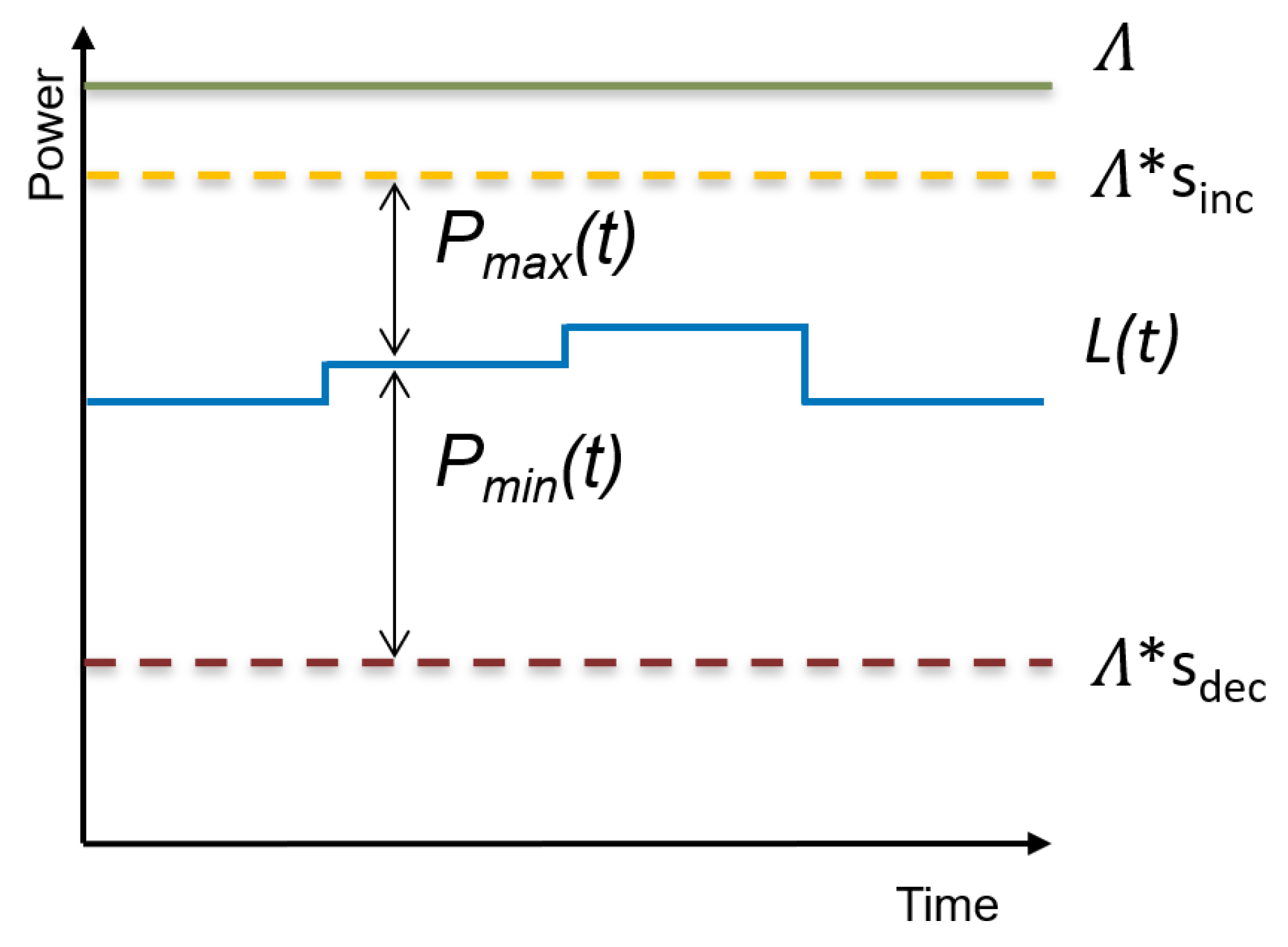
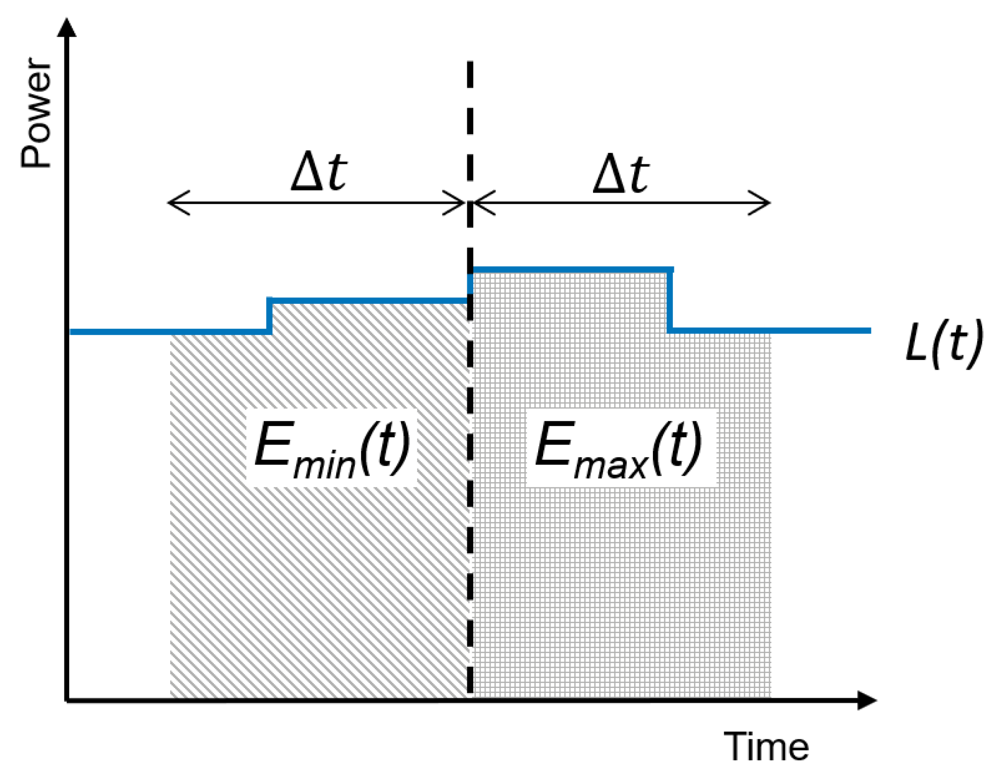
2.2.2. Boundary Conditions for the DR Implementation

The aggregated DR potential time series per grid node, $P_{max}^{i,t}$, $P_{min}^{i,t}$, $E_{max}^{i,t}$ and $E_{min}^{i,t}$ (Section 2.1), served as boundary conditions for the optimisation. First, the time series were normalised to per-unit values, using the maximum values of the $P_{max}^{i,t}$ and $E_{max}^{i,t}$ time series:

$$\begin{array}{c}\hfill p_{min,pu}^{i,t}=P_{min}^{i,t}/\underset{0\le t\le 8760}{max}{P}_{max}^{i,t}\forall i,t\end{array}$$

(16)

$$\begin{array}{c}\hfill p_{max,pu}^{i,t}=P_{max}^{i,t}/\underset{0\le t\le 8760}{max}{P}_{max}^{i,t}\forall i,t\end{array}$$

(17)

$$\begin{array}{c}\hfill e_{min,pu}^{i,t}=E_{min}^{i,t}/\underset{0\le t\le 8760}{max}{E}_{max}^{i,t}\forall i,t\end{array}$$

(18)

$$\begin{array}{c}\hfill e_{max,pu}^{i,t}=E_{max}^{i,t}/\underset{0\le t\le 8760}{max}{E}_{max}^{i,t}\forall i,t\end{array}$$

(19)

The boundary conditions were then defined as follows:

$$\begin{array}{cc}\hfill P_{inst}^i& \le \underset{0\le t\le 8760}{max}{P}_{max}^{i,t}\forall i,\hfill \end{array}$$

(20)

$$\begin{array}{cc}\hfill P_{inst}^i·p_{min,pu}^{i,t}& \le P^{i,t}\le P_{inst}^i·p_{max,pu}^{i,t}\forall i,t,\hfill \end{array}$$

(21)

$$\begin{array}{cc}\hfill E_{inst}^i·e_{min,pu}^{i,t}& \le E^{i,t}\le E_{inst}^i·e_{max,pu}^{i,t}\forall i,t.\hfill \end{array}$$

(22)

$E_{inst}^i$ was not an optimisation variable, but depended on $P_{inst}^i$ via:

$$\begin{array}{c}\hfill P_{inst}^i/\underset{0\le t\le 8760}{max}{P}_{max}^{i,t}=E_{inst}^i/\underset{0\le t\le 8760}{max}{E}_{max}^{i,t}\forall i.\end{array}$$

(23)

The optimised $P^{i,t}$ time series for each grid node were used as input data for the optimisation at the regional level, which is described in the next section.

2.3. Optimisation at the Regional Level

In the optimisation at the regional level, the DR expansion and dispatch was optimised per grid node. This was implemented as part of this work in a one-node model, separate from eTraGo, but also based on PyPSA [32]. As the computational times were lower in this step, no aggregation was needed, and all 19 DR technologies were considered. In this case, the DR potential times series per grid node for each individual technology, $P_{max}^{c,i,t}$, $P_{min}^{c,i,t}$, $E_{max}^{c,i,t}$ and $E_{min}^{c,i,t}$ were used as boundary conditions for the optimisation. First, the time series were normalised to per-unit values, using the maximum values of the $P_{max}^{c,i,t}$ and $E_{max}^{c,i,t}$ time series:

$$\begin{array}{c}\hfill p_{min,pu}^{c,i,t}=P_{min}^{c,i,t}/\underset{0\le t\le 8760}{max}{P}_{max}^{c,i,t}\forall c,i,t\end{array}$$

(24)

$$\begin{array}{c}\hfill p_{max,pu}^{c,i,t}=P_{max}^{c,i,t}/\underset{0\le t\le 8760}{max}{P}_{max}^{c,i,t}\forall c,i,t\end{array}$$

(25)

$$\begin{array}{c}\hfill e_{min,pu}^{c,i,t}=E_{min}^{c,i,t}/\underset{0\le t\le 8760}{max}{E}_{max}^{c,i,t}\forall c,i,t\end{array}$$

(26)

$$\begin{array}{c}\hfill e_{max,pu}^{c,i,t}=E_{max}^{c,i,t}/\underset{0\le t\le 8760}{max}{E}_{max}^{c,i,t}\forall c,i,t\end{array}$$

(27)

The boundary conditions were then defined as follows:

$$\begin{array}{cc}\hfill P_{inst}^{c,i}& \le \underset{0\le t\le 8760}{max}{P}_{max}^{c,i,t}\forall c,i,\hfill \end{array}$$

(28)

$$\begin{array}{cc}\hfill P_{inst}^{c,i}·p_{min,pu}^{c,i,t}& \le P^{c,i,t}\le P_{inst}^{c,i}·p_{max,pu}^{c,i,t}\forall c,i,t,\hfill \end{array}$$

(29)

$$\begin{array}{cc}\hfill E_{inst}^{c,i}·e_{min,pu}^{c,i,t}& \le E^{c,i,t}\le E_{inst}^{c,i}·e_{max,pu}^{c,i,t}\forall c,i,t.\hfill \end{array}$$

(30)

$E_{inst}^{c,i}$ was not an optimisation variable, but depended on $P_{inst}^{c,i}$ via:

$$\begin{array}{c}\hfill P_{inst}^{c,i}/\underset{0\le t\le 8760}{max}{P}_{max}^{c,i,t}=E_{inst}^{c,i}/\underset{0\le t\le 8760}{max}{E}_{max}^{c,i,t}\forall c,i.\end{array}$$

(31)

Further, the sum of the DR dispatch of all technologies needed to match the aggregated DR dispatch time series at each grid node that resulted from the optimisation at the national level:

$$\begin{array}{c}\hfill P^{i,t}=\sum _c{P}^{c,i,t}\forall c,i,t.\end{array}$$

(32)

The target of the optimisation at the regional level was to minimise the costs of the DR installation and operation at each grid node, considering investment and variable costs:

$$\underset{\begin{array}{c}{P}_{inst}^{c,i},P^{c,i,t}\end{array}}{min}\left[\sum _c(P_{inst}^{c,i}·c_{inv,an}^c+\sum _t{\left[P^{c,i,t}\right]}^{+}·c_{var}^c)\right].$$

(33)

2.4. Economic Assessment

The economic assessment was carried out, both for the aggregated DR units that were considered in the optimisation at the national level and for the individual DR technologies that were considered in the optimisation at the regional level. For the economic assessment of the aggregated DR units, the installed DR capacities $P_{inst}^i$ and DR dispatch time series $P^{i,t}$ for each grid node, as well as the cost parameters, were used as input data. The net present value (NPV) [23] was calculated for the aggregated DR units at each grid node:

$$\begin{array}{cc}\hfill & NP{V}^i=-P_{inst}^i·c_{inv}^i+\sum _{p=1}^{15}{R}_p^i/{(1+d)}^p,\hfill \end{array}$$

(34)

$$\begin{array}{cc}\hfill & R_p^i=-c_{fix}^i+\sum _t{\left[P^{i,t}\right]}^{+}·(r-c_{var}^i).\hfill \end{array}$$

(35)

$R_p^i$ was the net cash inflow minus outflows for one year and was made up by the fixed costs, the variable costs and the revenue r for applying DR (see explanation below). For the technology-specific economic assessment based on the optimisation at the regional level, the NPV was calculated similarly, but the input data for the respective technologies, c, were used:

$$\begin{array}{cc}\hfill & NP{V}^{c,i}=-P_{inst}^{c,i}·c_{inv}^c+\sum _{p=1}^{15}{R}_p^{c,i}/{(1+d)}^p,\hfill \end{array}$$

(36)

$$\begin{array}{cc}\hfill & R_p^{c,i}=-c_{fix}^c+\sum _t{\left[P^{c,i,t}\right]}^{+}·(r-c_{var}^c).\hfill \end{array}$$

(37)

For a better comparison, the specific net present values were calculated by dividing by the installed capacities:

$$\begin{array}{cc}\hfill & np{v}^i=NP{V}^i/P_{inst}^i,\hfill \end{array}$$

(38)

$$\begin{array}{cc}\hfill & np{v}^{c,i}=NP{V}^{c,i}/P_{inst}^{c,i}.\hfill \end{array}$$

(39)

In Germany, there are different options to generate revenue by applying DR [35], arbitrage in electricity markets [36], contracts with the grid operator or participation in auctions with the target to avoid grid congestion, provide operating reserve and provide balancing energy for the balancing group. However, due to several obstacles and low margins in the different markets, DR has rarely been used in Germany up to now [37]. Several studies [37] have recommended changing the circumstances for DR, e.g., the regulatory framework, to improve the economic viability and to allow the utilisation of the potential of DR for renewable energy integration. Against this backdrop, we did not use a fixed value for the possible revenue of DR, r, but conducted a case study for values between 15 EUR/MWh and 25 EUR/MWh.

As described in Section 2.1, the DR investment costs are mainly caused by the ICT components for making the loads controllable, e.g., a smart meter gateway [26]. However, such ICT components may not only be used for DR, but may also lead to other benefits, for example an increased energy efficiency due to a higher consumer awareness of the real-time energy demand [38]. In Germany, since 2020, grid operators are obliged to equip electricity consumers of specific demand categories with a smart meter [39]. For these reasons, it is questionable to what extent the above-mentioned ICT investment costs can be assigned exclusively to the application of DR. Thus, we considered two cases in this work: (1) full investment costs consideration for DR, as introduced in Section 2.1 and (2) zero investment cost for DR (only variable costs are considered).

3. Results and Discussion

In this section, we describe the results of the DR investment and dispatch optimisation at the national level (Section 3.1), as well as at the regional level (Section 3.2). The economic assessment is presented in Section 3.3. In Section 3.4, the sensitivity of the results on different input parameters is analysed.

3.1. Optimisation at the National Level

For the optimisation at the national level, we first considered the temporal dimension by analysing the dispatch of the aggregated DR units. Second, we considered the spatial dimension by analysing the allocation of aggregated DR units within the German power grid.

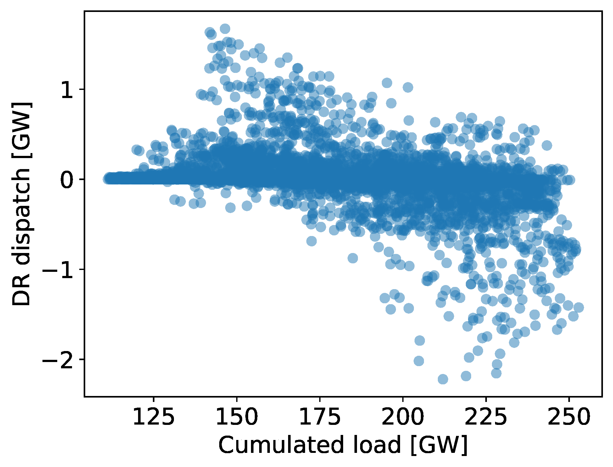
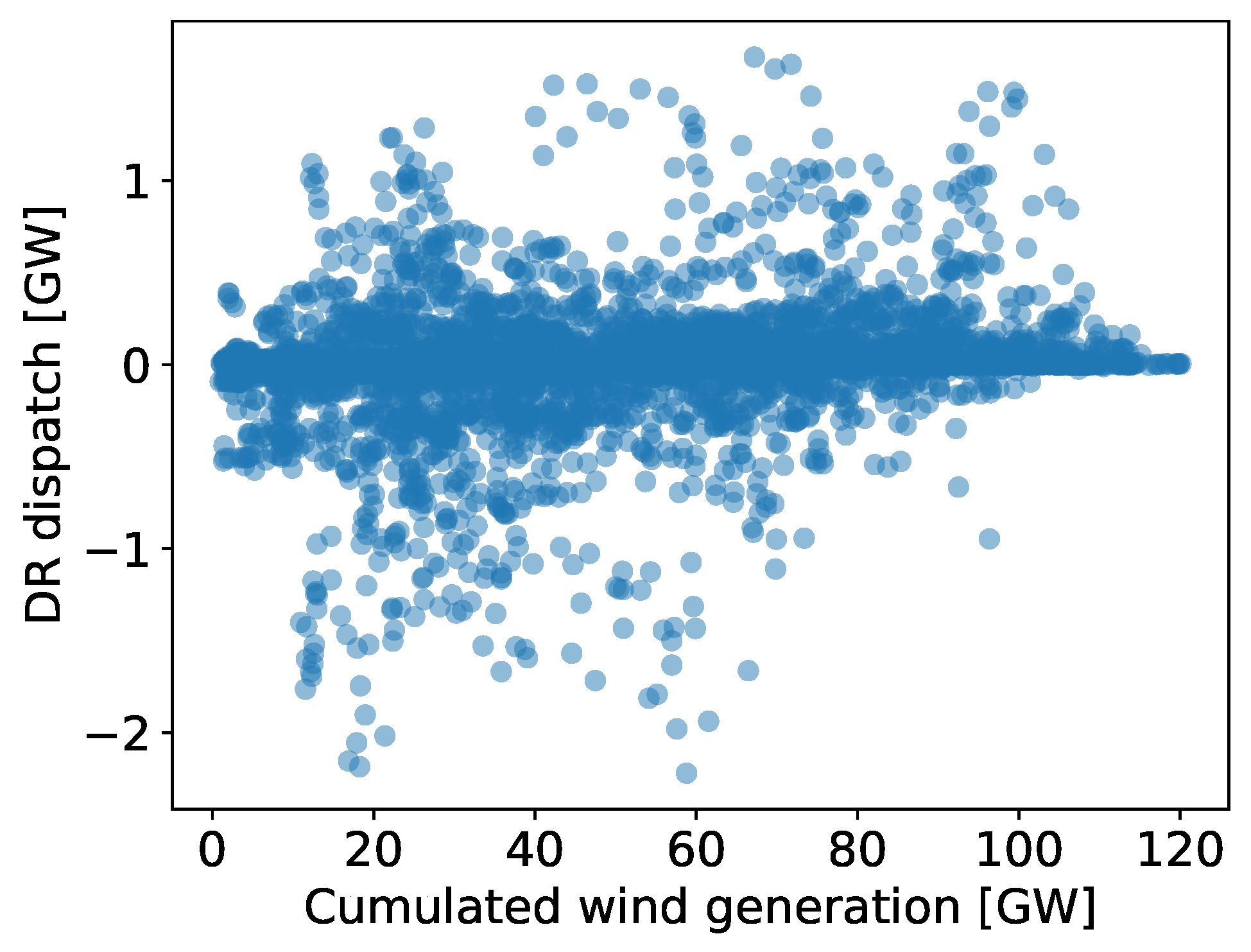
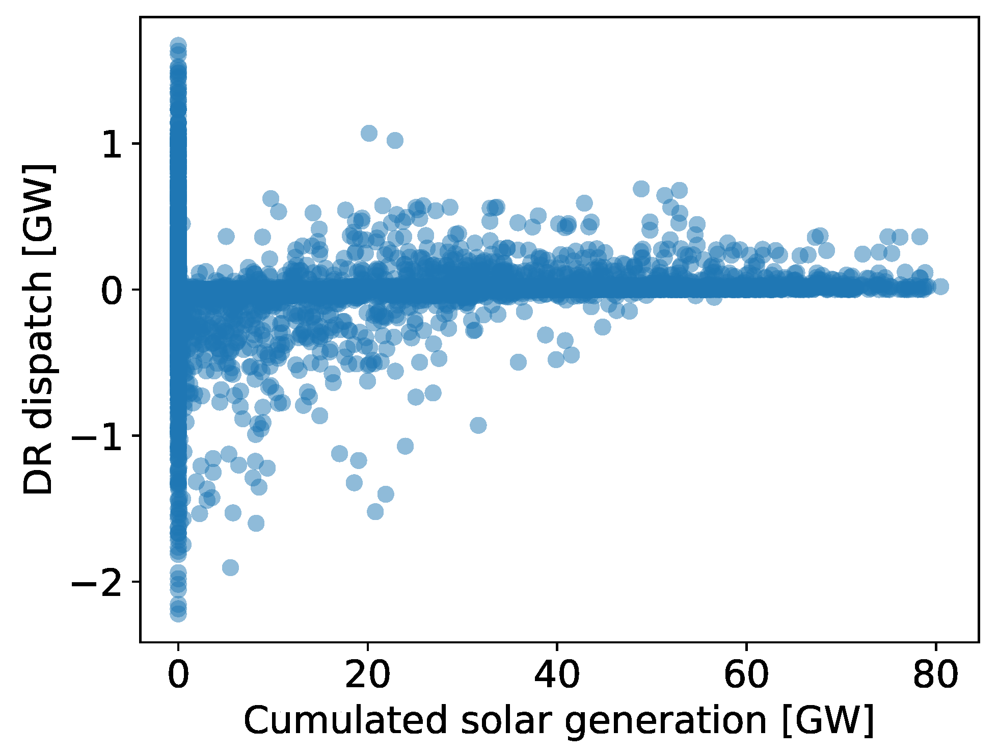
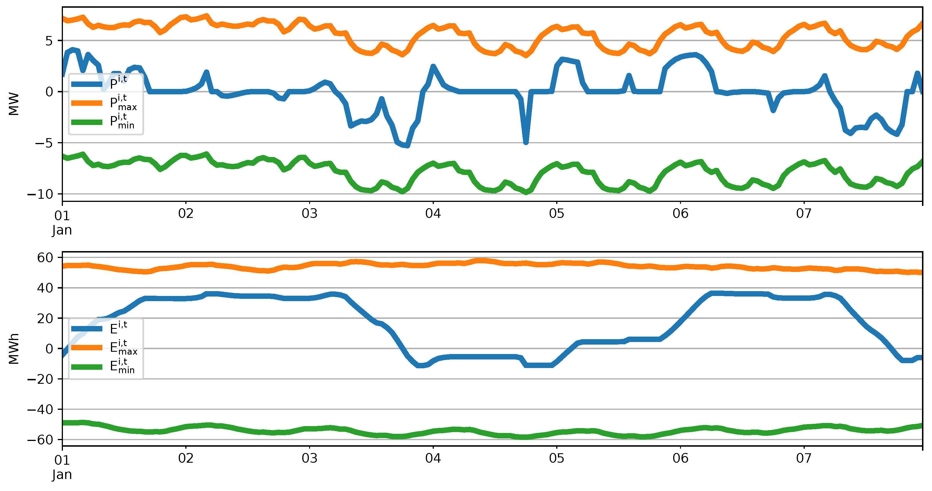
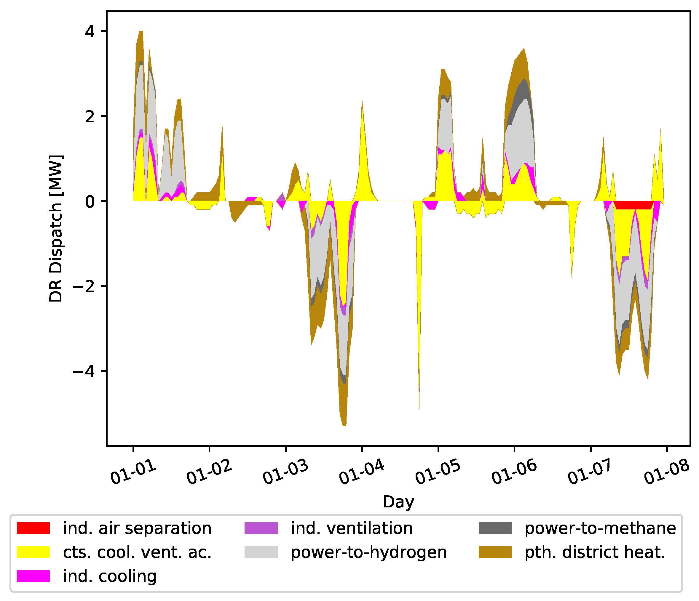
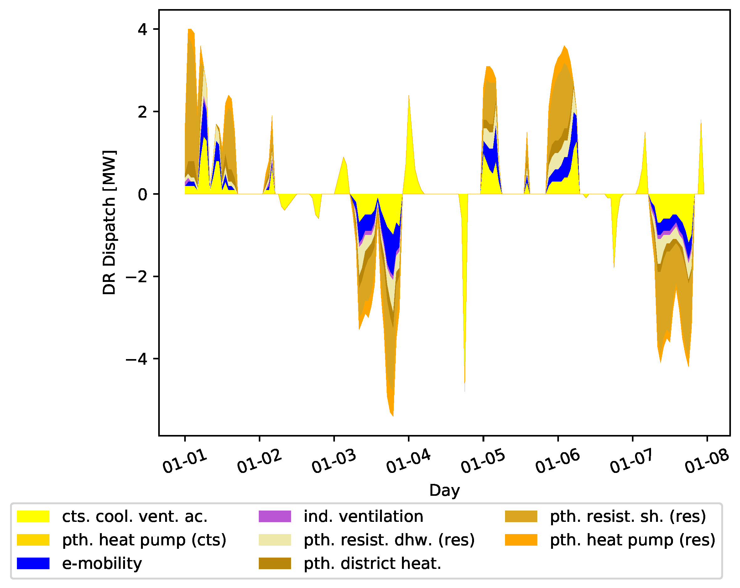
3.1.1. DR Dispatch Analysis

To determine the main drivers of the DR dispatch, we analysed the correlations with wind generation, solar generation and the cumulated load at each time step t of the year. The strongest correlation was present between the DR dispatch and the total system load, with a Pearson correlation coefficient of $R=-0.31$. The correlation was negative because the storage-equivalent DR units were charged at a low system load and discharged (negative value) at a high system load, as shown in Figure 4. Wind and solar generation both showed a lower correlation with the DR dispatch, with a value of $R=0.14$ for wind and $R=0.05$ for solar generation, as shown in Figure 5 and Figure 6. Both values were positive because the storage equivalent DR units were charged at times of high solar and wind generation and discharged (negative values) at times of low generation.

Figure 7 (top row) shows the optimised DR dispatch, $P^{i,t}$, for the first week of the year for a transmission grid node near the city of Dortmund in the west of Germany, as an example.

Furthermore, the figure illustrates that the DR dispatch stayed within the boundary conditions set by the maximum load increase $P_{max}^{i,t}$ and load decrease $P_{min}^{i,t}$ (Equation (21)). During the first day of the week there were multiple load increases of up to 4 MW, which led to an increase of the filling level of the storage-equivalent DR operation $E^{i,t}$, as shown in Figure 7 (bottom row). During the second day, there were no significant load increases and decreases and $E^{i,t}$ stayed approximately constant. At the third day, there was a load decrease of up to $-5$ MW, leading to a reduction of the filling level.

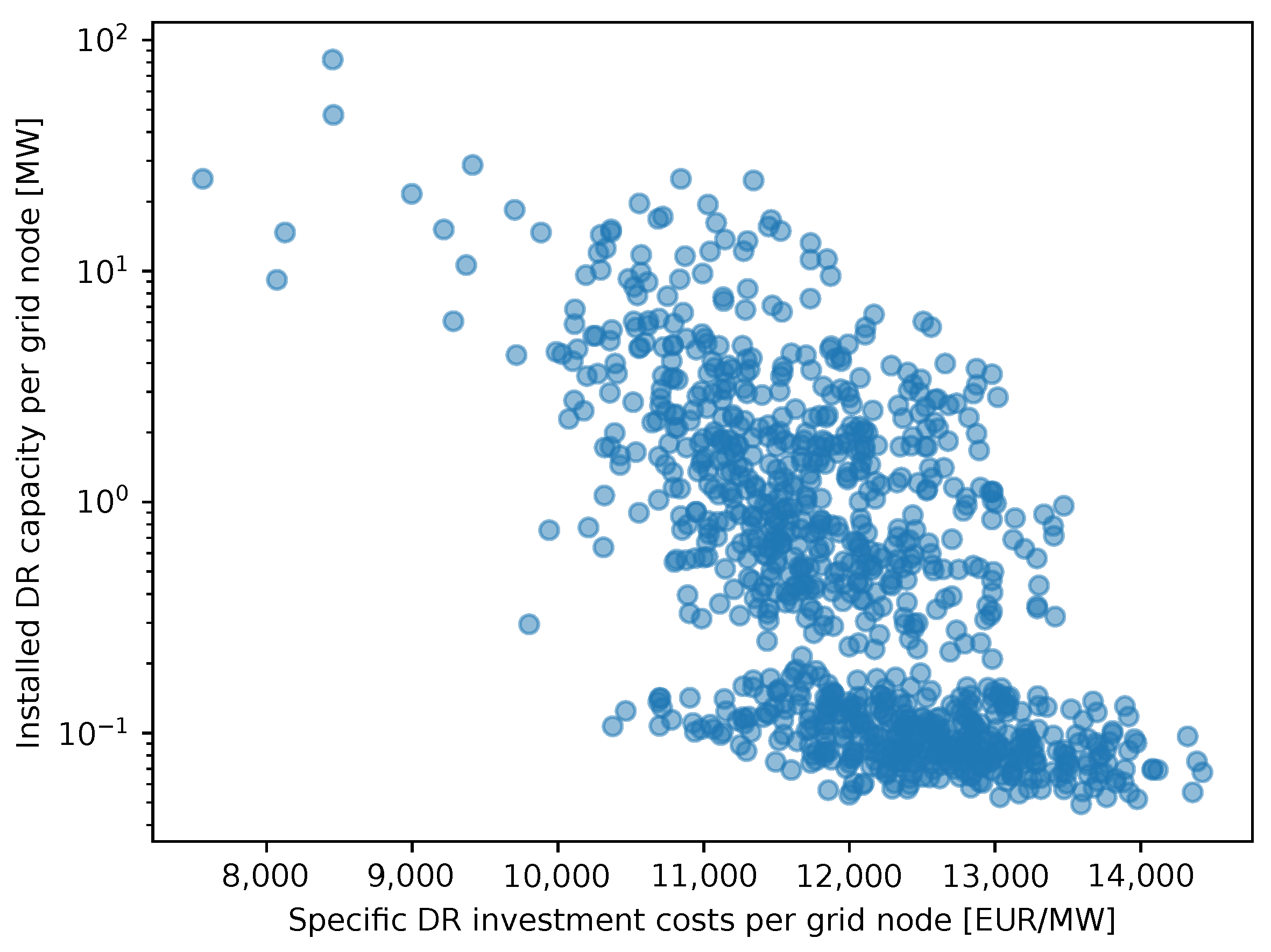
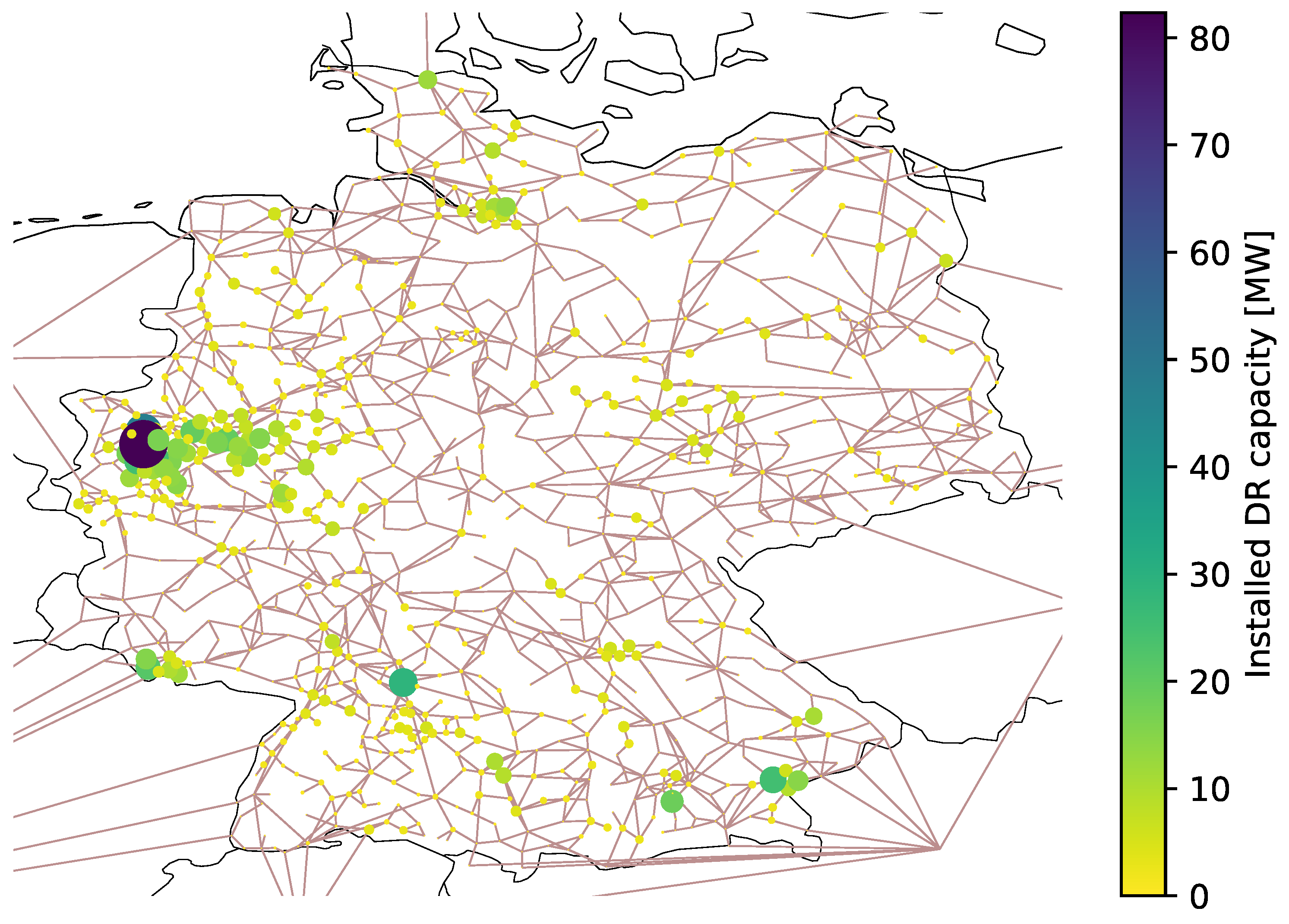
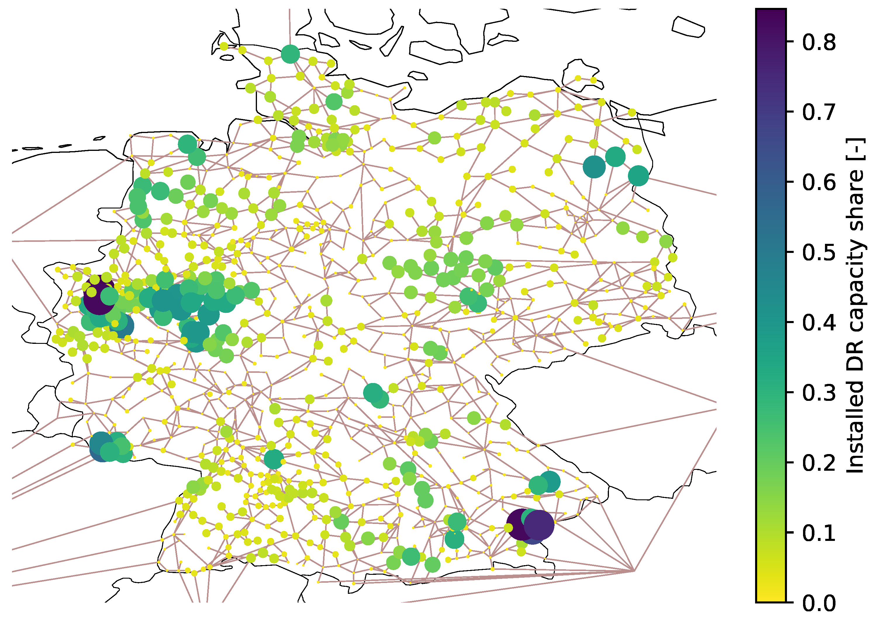
3.1.2. DR Allocation Analysis

To analyse the allocation of the DR units, we determined the Pearson correlation coefficient, R, for the DR expansion per transmission grid node with the average DR investment costs per grid node, the average loading of the lines connected to the grid node and the average cumulated load per grid node. The highest correlation was present for the DR investment costs per grid node with a value of $R=-0.47$ (see Figure 8), followed by the correlation with the average load per grid node with $R=0.31$ and the correlation with the average line loading with the lowest value of $R=0.04$ (not illustrated in a dedicated figure).

Figure 9 shows the spatial allocation of the aggregated DR units in Germany, as optimised by eTraGo. In the west of Germany, there was one large unit of 82 MW installed, as well as several medium-sized units in the range of 10–50 MW. Furthermore, there were 15 medium sized DR units spread across Germany and approximately 200 with a size below 10 MW. One reason for the high expansion of DR units in the west of Germany was that there was also the most DR potential available in that region due to the high population density and the existing heavy industry [25].

Figure 10 shows the share of the installed DR capacity in the total DR potential per grid node.

In addition, the relative DR capacity expansion in the west of Germany was high with more than $40\%$ at multiple grid nodes. However, in the rest of Germany as well, there was a significant number of grid nodes with a high relative DR expansion of up to $80\%$.

There was also a noticeable high DR expansion in several border regions to neighbouring countries. While there were 380 kV power lines located in most other border crossings, there were 220 kV power lines with a lower capacity present in those border regions with a high DR expansion (220 kV power lines at border crossings: Ensdorf–Saint Avold, Neuenhagen–Vierraden, Pleinting–St. Peter). Such a lower line capacity can lead to a higher line loading. Additionally, the neighbouring countries were abstracted by one node each in the model, which may also have increased the loading of specific lines at border crossing lines. As a consequence, the optimiser may have installed DR units in such locations to avoid line overloading.

3.2. Optimisation at the Regional Level

In the optimisation at the regional level, we investigated which of the considered DR technologies were installed and how they were dispatched. We used the transmission grid node near the city of Dortmund as the same example that was already considered in Section 3.1.1, because a high number of DR technologies were installed there, as a result of the optimisation.

In Figure 11, the case that considered investment costs is depicted, yielding that only large scale technologies were applied that had low specific investment costs (≤10 TEUR/MW) for enabling DR: air separation, cooling, ventilation and AC processes in commercial, trade and services (CTS-AC), industrial ventilation, industrial cooling, power-to-hydrogen, power-to-methane and power-to-heat in district heating.

Out of these technologies, CTS-AC had the lowest variable costs and was thus used nearly each time DR was applied. However, at most time steps, the capacity of CTS-AC was not sufficient to cover the required load increase or decrease as determined by the optimisation at the national level. Thus, the DR of power-to-hydrogen and power-to-heat in district heating was also significantly used. Air separation, industrial ventilation, industrial cooling and power-to-methane played a minor role due to the limited available potential in the area surrounding the regarded grid node [25].

Figure 12 shows the case without DR investment costs. Beneath CTS-AC and industrial ventilation, several small-scale DR technologies were used in this case due to the low variable costs. Residential power-to-heat contributed the largest part, followed by e-mobility.

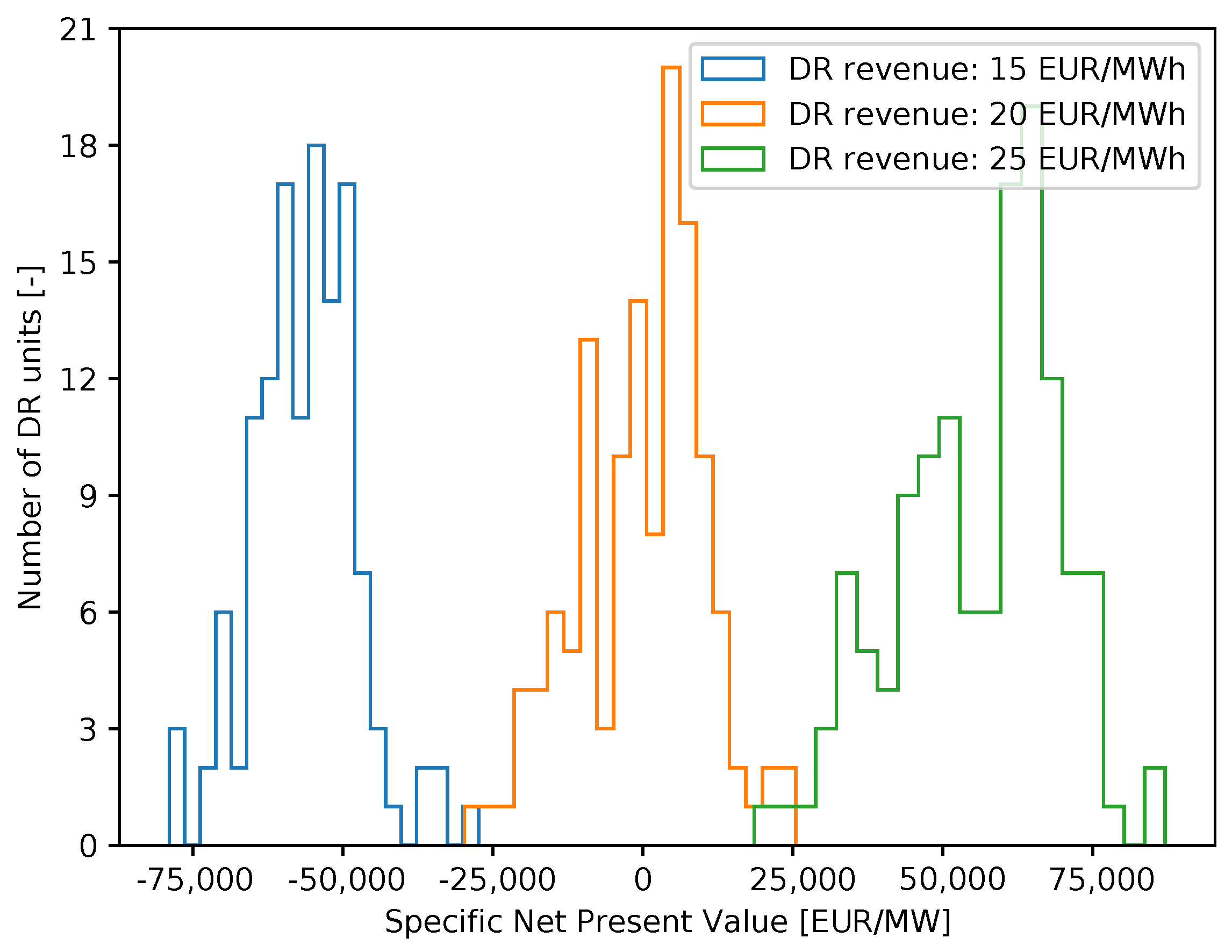
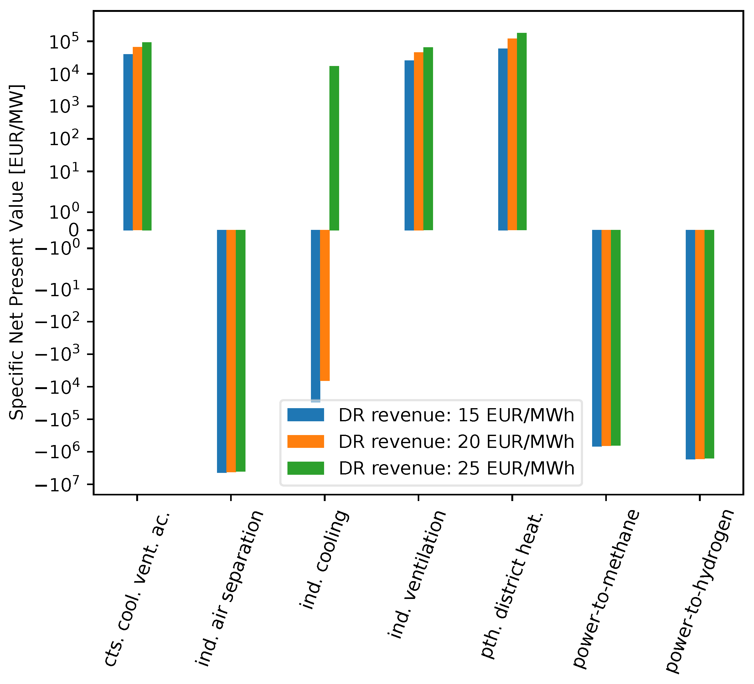
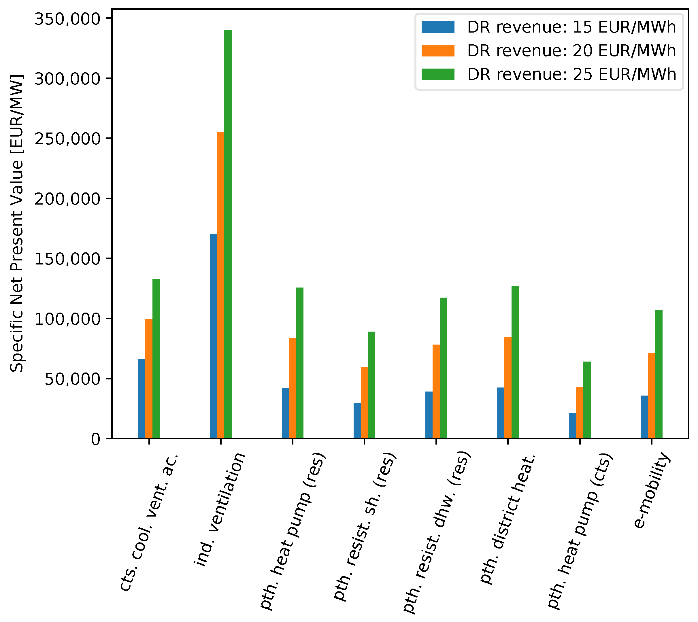
3.3. Economic Assessment

In this section, we describe the results of the economic assessment for the aggregated DR units that were used in the optimisation at the national level and for the individual DR technologies that were considered in the optimisation at the regional level.

Figure 13 illustrates the frequency distribution of the specific NPVs per aggregated DR unit per grid node, considering three different DR revenue scenarios.

For clarity, only the aggregated DR units with an installed capacity larger than $0.1$ MW were taken into account. While for the DR revenue of 15 EUR/MWh, the specific NPVs were negative for all considered units, for the DR revenue of 25 EUR/MWh all specific NPVs were positive and ranged between 18 TEUR/MW and 85 TEUR/MW. For the DR revenue of 20 EUR/MWh, about the half of the DR units had negative NPVs and the other half had positive NPVs.

The resulting specific NPV values for the different technologies for the example of a grid node near the city of Dortmund are shown in Figure 14 and Figure 15 for different revenue scenarios.

For the case that considered investment costs, PtH in district heating had the highest specific NPV, with 180 TEUR/MW for the revenue scenario with 25 EUR/MWh, followed by CTS-AC, with 90 TEUR/MW, and industrial ventilation, with 65 TEUR/MW. For industrial cooling, the NPV switched from negative to positive between the revenue scenarios of 20 EUR/MWh and 25 EUR/MWh. Air separation, power-to-methane and power-to-hydrogen all had negative NPVs, as their variable costs were higher than the assumed revenue for all revenue scenarios. Thus, these technologies were chosen by the optimisation at the regional level to cover the dispatch of the aggregated DR unit set by the optimisation at the national level at their respective grid node. For possible operators though, it would not be economically viable to apply these technologies for DR. However, as discussed in Section 3.5, further research is required to derive more reliable parameters for the variable costs of DR by power-to-gas plants.

In the case without investment cost consideration (Figure 15), there were no technologies with a negative NPV. The industrial ventilation technology had the highest specific NPV with 340 TEUR/MW for the revenue scenario with 25 EUR/MWh. The reason for this is that it had low variable costs of 5 EUR/MWh and a low available load increase potential, $P_{max}=0.52$ MW, being fully used multiple times, which led to a high specific NPV. The other utilised technologies all had specific NPV values between 50 and 150 TEUR/MW, because they all had variable costs of 5 or 10 EUR/MWh.

3.4. Sensitivity Analysis

In this section different influences on the results are analysed: the spatial and temporal energy system model resolution, the technological detail of the model (for the example of heat pump size classes) and the applied weather year, as well as uncertainties in the open-source power grid model and cost parameters.

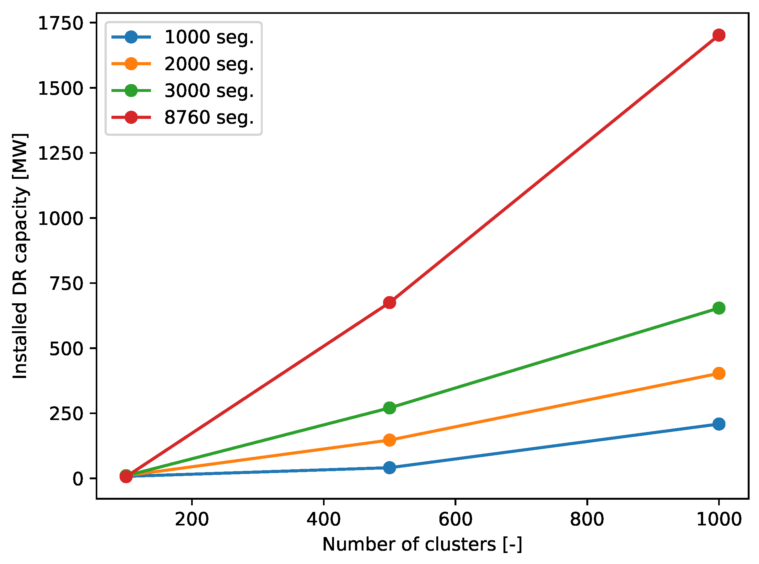
3.4.1. Influence of Spatial and Temporal Energy System Model Resolution

In this work, a comparably high spatial resolution of 1000 nodes for the German power grid model was applied. Thus, in this section, we analyse the influence on the installed DR capacity of using a lower spatial resolution of 500 and 100 grid nodes. The k-means algorithm was applied to reduce the number of nodes in the power grid model, as introduced in Section 2.2.1. Furthermore, we investigated the influence of using a lower temporal resolution of 5000, 2000 and 1000 time steps. For that, we used the segmentation clustering algorithm [40], which clustered adjacent hours to one hour (called segments), based on the implementation in [41].

As shown in Figure 16, for the case with 100 grid node clusters, there was nearly no installed DR capacity, no matter which number of time segments were used.

For the case with 500 grid node clusters, the installed DR capacity for Germany as a whole rose from 40 MW for 1000 time segments to 680 MW for 8760 time segments. For the case with 1000 grid node clusters, the installed DR capacity ranged between 210 MW for 1000 time segments and 1700 MW for 8760 time segments. It can thus be concluded that both a higher temporal and spatial resolution of the energy system model led to a higher DR expansion. This is consistent with the results of Frysztacki et al. [24], who showed that a higher grid resolution revealed more bottlenecks in the power flow.

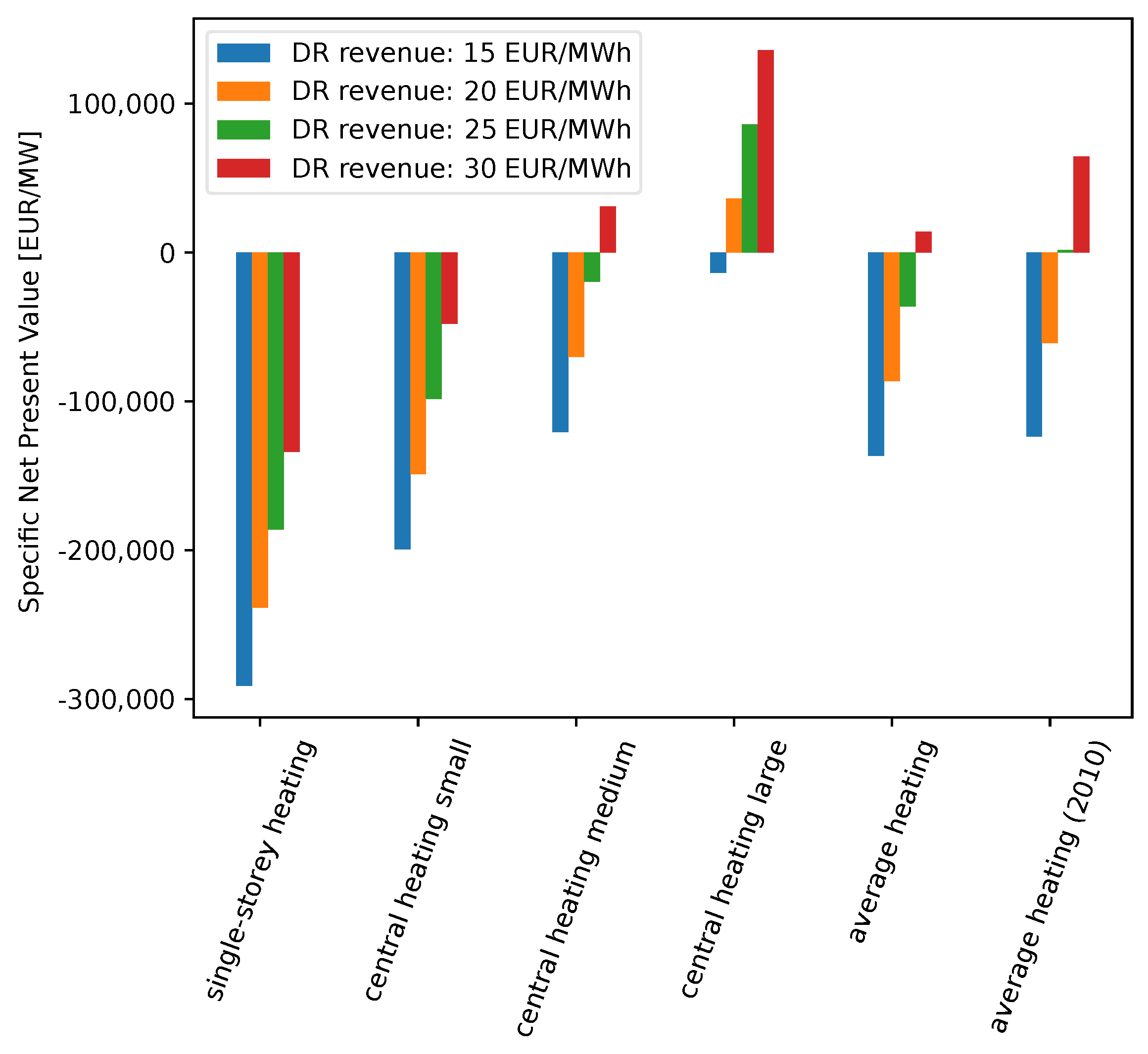
3.4.2. Influence of Heat Pump Size Classes and the Weather Year

In order to assess the influence of the technological detail of the model on the results for the NPV, we further differentiated between different heat pump size classes, as an example. In a prior work [42], we defined more than 700 residential building categories and assigned a heat demand value to each category. As shown in

Table 2. Investment costs for the flexibilisation of different heat pump size classes [25].

Heat Pump Size	${\mathit{P}}_{\mathbf{el}}$ (kW)	${\mathit{c}}_{\mathbf{inv}}$ (EUR/MW)
Single-storey heating	2.7	115,000
Central heating small	3.7	84,000
Central heating medium	5.5	57,000
Central heating large	14.2	22,000

, the buildings were grouped according to their heating types, single-storey heating and central heating. For the central heating technology, we distinguished between small-, medium- and large-size central heating systems. To determine the installed electric capacity, $P_{el}$, the heating capacity, ${\dot{Q}}_{inst}$, was divided by the annual average coefficient of performance of the electric heating, $<COP>$. We determined the regionalised DR potential time series and the specific investment costs for the different heat pump size classes in [25].

The influence of the heat pump size classes on the specific NPV is shown in Figure 17. For demonstration, we used a transmission grid node in the city of Hamburg in Northern Germany as an example, because heat pumps were used for DR in the optimisation at the regional level at this grid node to a large extent.

Due to the high specific investment costs for DR enablement, the single-storey heating, as well as the small central heating category had negative NPV values for all considered revenue scenarios. The medium central heating category had a positive specific NPV, with 31 TEUR/MW, only for the revenue scenario with 30 EUR/MWh. The large central heating category reached positive NPVs for the revenue scenarios with 20, 25 as well as 30 EUR/MWh, and the maximum specific NPV was 136 TEUR/MW. In comparison, the aggregated average heating had significantly higher specific NPVs than the single-storey heating, as well as the small central heating, and lower specific NPVs than the medium and large central heating. This yielded that it made a difference for the modelling results to take the heating size classes into account.

Furthermore, we investigated the influence of the weather year on the specific NPV. Therefore, the optimisation was repeated for the year 2010, which had a 1.7 °C lower average temperature than the year 2011 [43]. This yielded a higher heat demand, higher DR potential and higher specific NPVs. As shown in Figure 17, the specific NPV for the average heating category and, e.g., the DR revenue scenario with 30 EUR/MWh, was 51 TEUR/MW higher for 2010 than for 2011. Thus, for a reliable economic assessment of DR by heat pumps, multiple weather years should be taken into account.

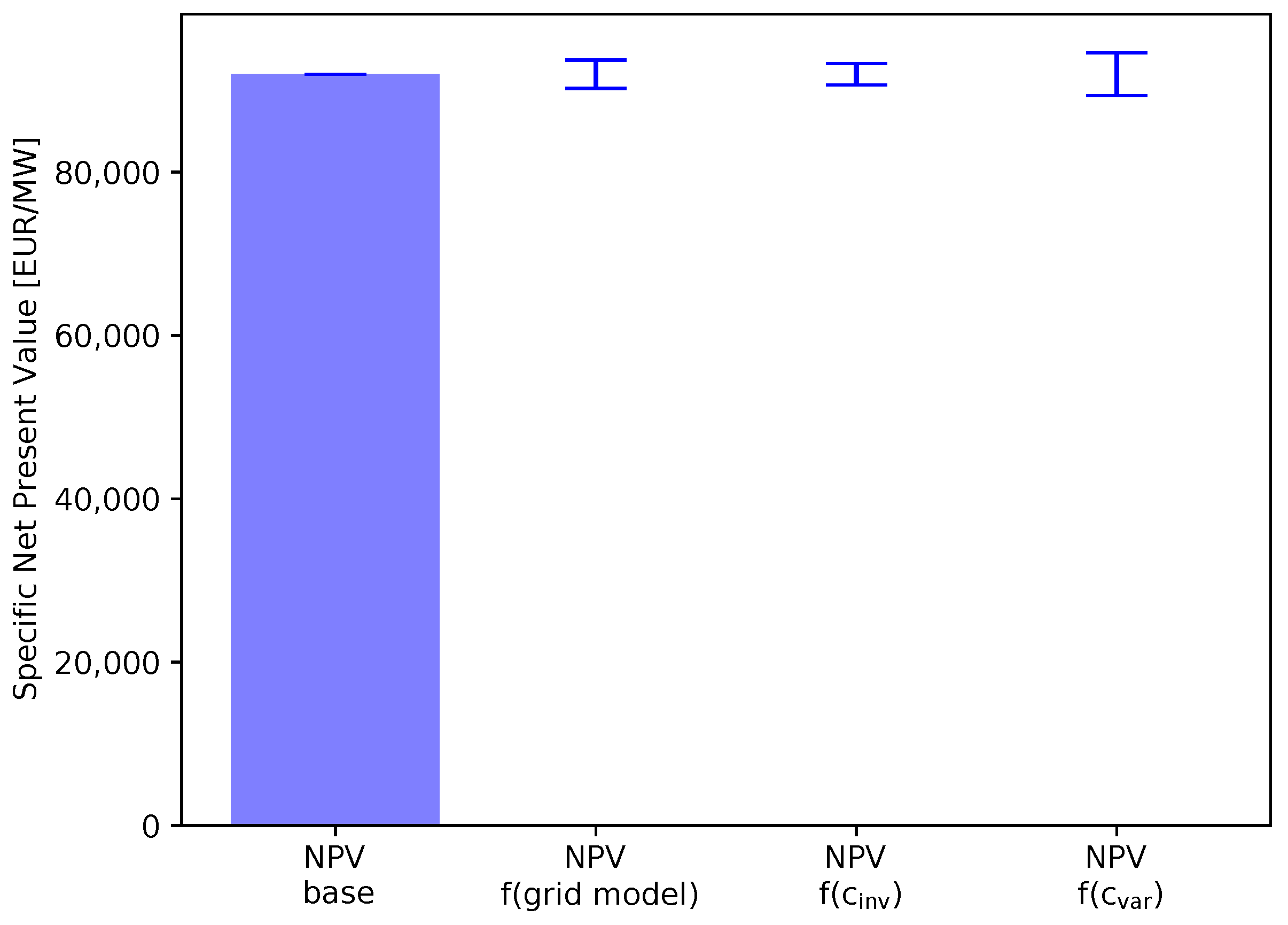
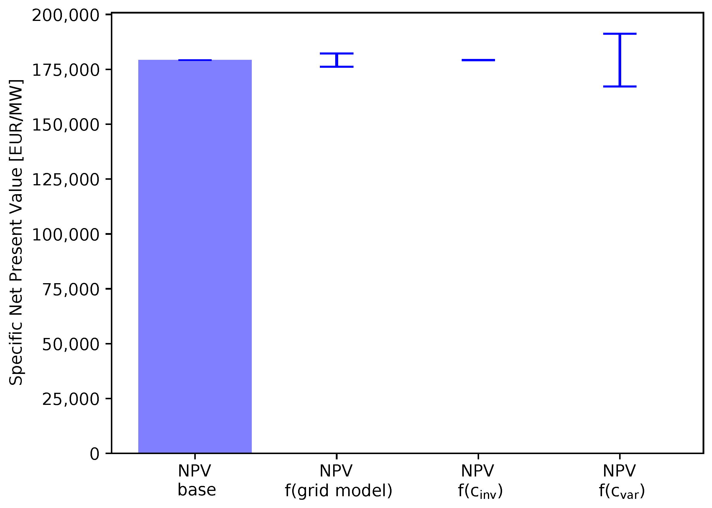
3.4.3. Influence of Uncertainties in the Open-Source Power Grid Model and Cost Parameters

The sensitivity of the specific NPV to uncertainties in the open-source power grid model, the DR investment costs and the DR variable costs are shown in Figure 18, for the example of the CTS-AC technology at a grid node close to the city of Dortmund, which was already used in Section 3.2.

In a previous work [44], we compared the power flow results of the open-source model eTraGo, which was used in this work, with a reference model of a grid operator, yielding errors of $\pm 1.7\%$. We assumed that this error led to a deviation of the DR utilisation of the same magnitude and repeated the economic assessment with a $\pm 1.7\%$ modified DR utilisation. This led to a $\pm 1.9\%$ change in the specific NPV.

According to [26], the uncertainty for the DR investment costs and variable costs can both be estimated at $\pm 10\%$. Repeating the economic assessment with the modified investment costs led to a $\pm 1.4\%$ change in the specific NPV. Modifying the variable costs by $\pm 10\%$ led to a $\pm 3\%$ change in the specific NPV (see Figure 18). The NPV was more sensitive to the variable costs, as the generated margins depended on the small difference between the variable costs and the DR revenue, which was overproportionally changed by a modification of the variable cost.

In Figure 19, the same modifications in the input parameters as described in the last paragraph were applied for the economic assessment of the PtH in district heating technology. While the influence of the grid model stayed approximately equal, the modification of the investment costs resulted in a negligible small change of the specific NPV, and the modification of the variable costs resulted in a significantly higher change of the specific NPV, with $\pm 6.7\%$. The reason for this was that the PtH in district heating technology had notably lower investment costs and higher variable costs than the CTS-AC technology, yielding a higher influence of the variable cost.

3.5. Critical Appraisal

In this section, we compare the results of the present work to literature values and comment on possible future improvements of the applied methodology and data. The result for the installed DR capacity added up to $1.7$ GW for Germany as a whole (see Section 3.4.1). In comparison, Steurer [26] obtained a higher installed DR capacity value of 8 GW for Germany. One reason for this difference can be that in [26], a scenario with $80\%$ share of renewable energies in the German power generation for 2050 was considered. This led to a higher flexibility demand as in the 2035 scenario with a $66\%$ renewable energy share in the present study. However, the resulting DR capacity yielded in this study should be assessed as a conservative value.

Our analysis yielded that the break-even point was reached at a DR revenue between 20–25 EUR/MWh in most cases, when considering aggregated DR units per grid node (Section 3.3). Moreover, the results for the optimisation at the regional level showed that there were several DR technologies that reached the break-even point at a revenue of 20–25 EUR/MWh. In Germany, there are low voltage grid operators that reduce network charges for controllable loads. On average, the reduction amounts to 37 EUR/MWh [45]. These controllable loads are mostly night storage heaters and are rather used for smoothing the load to adjust it to conventional power plant dispatch, than for avoiding VRE curtailment [45]. However, it can be summarised that the yielded break-even revenue range of 20–25 EUR/MWh is close to the average network charge reduction of 37 EUR/MWh and seems a plausible value.

The economic viability of DR strongly depends on the assumed investment and variable cost parameters, which are partly associated with high uncertainties. The PtG technology for example is not widely used yet and no variable costs for DR with PtG could be identified. Thus, the variable costs were adopted from the air separation technology [25]. In order to obtain a more reliable economic assessment, further research on DR cost parameters is required.

4. Conclusions and Outlook

In this work, we assessed the economic viability of demand response using a high spatially and temporally resolved energy system model for Germany, coupled with a regional DR optimisation model considering 19 DR technologies.

Our analysis yielded a high sensitivity of the power grid resolution on the installed DR capacity, which indicated power grid bottlenecks to drive the DR expansion. However, the DR units were not only installed close to locations of high renewable energy capacity that may cause line overloading. Instead, there was a rather equal distribution over all of Germany, with most DR units having an aggregated capacity of below 50 MW per grid node. The highest capacity was present in regions of low DR investment costs, e.g., due to industrial concentration.

On average, the break-even point for the DR units was reached at a DR revenue of 20–25 EUR/MWh. This range was of similar magnitude as the reduction in network charges that several low-voltage grid operators grant for controllable loads. In a scenario with full DR cost consideration, only large-scale technologies with low specific investment costs were applied. Air-conditioning processes in the commercial, trade and services sector were most utilised due to their low variable costs. Power-to-heat in district heating reached the highest net present value with 180 TEUR/MW during a period of 15 years and a revenue scenario of 25 EUR/MWh. In a scenario without investment costs considered, several small-scale technologies were used due to low variable costs. Residential power-to-heat was utilised most, followed by e-mobility. The net present values ranged from 50 to 340 TEUR/MW. The influence of the technological detail of the model was analysed for the example of DR with heat pumps. Taking different heat pump size classes into account led to differences in the net present value of more than 100 TEUR/MW compared to the simplified average heating category.

The economic viability of DR also depends on the applied input parameters for the economic assessment. Further studies are required to derive more precise parameters, e.g., for the investment and variable costs of DR.

References

1. Li, L.; Lin, J.; Wu, N.; Xie, S.; Meng, C.; Zheng, Y.; Wang, X.; Zhao, Y. Review and outlook on the international renewable energy development. Energy Built Environ. 2020, 3, 139–157. [Google Scholar] [CrossRef]
2. Shahzad, F.; Fareed, Z. Examining the relationship between fiscal decentralization, renewable energy intensity, and carbon footprints in Canada by using the newly constructed bootstrap Fourier Granger causality test in quantile. Environ. Sci. Pollut. Res. 2022, 1–10. [Google Scholar] [CrossRef] [PubMed]
3. European Commission. Amendment to the Renewable Energy Directive to Implement the Ambition of the New 2030 Climate Target; European Commission: Brusseles, Belgium, 2021; Available online: https://ec.europa.eu/info/sites/default/files/amendment-renewable-energy-directive-2030-climate-target-with-annexes_en.pdf (accessed on 27 September 2022).
4. Luz, T.; Moura, P. 100 Percent Renewable energy planning with complementarity and flexibility based on a multi-objective assessment. Appl. Energy 2019, 255, 113819. [Google Scholar] [CrossRef]
5. Christian, D.; Anna, G. Integration of Renewable Energy by Distributed Energy Storages. In Advances in Energy Storage: Latest Developments from R&D to the Market; Wiley: Hoboken, NJ, USA, 2022; pp. 839–850. [Google Scholar]
6. Shafiekhani, M.; Ahmadi, A.; Homaee, O.; Shafie-khah, M.; Catalão, J.P. Optimal bidding strategy of a renewable-based virtual power plant including wind and solar units and dispatchable loads. Energy 2022, 239, 122379. [Google Scholar] [CrossRef]
7. Cai, Q.; Xu, Q.; Qing, J.; Shi, G.; Liang, Q.M. Promoting wind and photovoltaics renewable energy integration through demand response: Dynamic pricing mechanism design and economic analysis for smart residential communities. Energy 2022, 261, 125293. [Google Scholar] [CrossRef]
8. Zöphel, C.; Schreiber, S.; Müller, T.; Möst, D. Which flexibility options facilitate the integration of intermittent renewable energy sources in electricity systems? Curr. Sustain. Energy Rep. 2018, 5, 37–44. [Google Scholar] [CrossRef]
9. Valdes, J.; González, A.B.P.; Camargo, L.R.; Fenández, M.V.; Macia, Y.M.; Dorner, W. Industry, flexibility, and demand response: Applying German energy transition lessons in Chile. Energy Res. Soc. Sci. 2019, 54, 12–25. [Google Scholar] [CrossRef]
10. Misconel, S.; Zöphel, C.; Möst, D. Assessing the value of demand response in a decarbonized energy system—A large-scale model application. Appl. Energy 2021, 299, 117326. [Google Scholar] [CrossRef]
11. Gils, H.C. Balancing of Intermittent Renewable Power Generation by Demand Response and Thermal Energy Storage. Ph.D. Thesis, University of Stuttgart, Stuttgart, Germany, 2015. [Google Scholar]
12. Paulus, M.; Borggrefe, F. The potential of demand-side management in energy-intensive industries for electricity markets in Germany. Appl. Energy 2011, 88, 432–441. [Google Scholar] [CrossRef]
13. Mueller, T.; Moest, D. Demand Response Potential: Available when Needed? Energy Policy 2018, 115, 181–198. [Google Scholar] [CrossRef]
14. Kies, A.; Schyska, B.U.; Von Bremen, L. The demand side management potential to balance a highly renewable European power system. Energies 2016, 9, 955. [Google Scholar] [CrossRef] [Green Version]
15. Kirkerud, J.; Nagel, N.O.; Bolkesjø, T. The role of demand response in the future renewable northern European energy system. Energy 2021, 235, 121336. [Google Scholar] [CrossRef]
16. Gils, H.C. Economic potential for future demand response in Germany–Modeling approach and case study. Appl. Energy 2016, 162, 401–415. [Google Scholar] [CrossRef] [Green Version]
17. Gangale, F.; Vasiljevska, J.; Covrig, C.F.; Mengolini, A.; Fulli, G. Smart Grid Projects Outlook 2017: Facts, Figures and Trends in Europe; Joint Research Centre of the European Commission: Petten, The Netherlands, 2017. [Google Scholar] [CrossRef]
18. Filusch, T.; Heilmann, A.; Lange, M.; Linnemann, J.; Erfurth, J.; Klug, S. Industrielle Lasten: Auf Dem Weg in die CO2-Neutrale Produktion. Enera Projektkompendium. 2021. Available online: https://projekt-enera.de/wp-content/uploads/enera-projektkompendium.pdf (accessed on 27 September 2022).
19. Meyer, T. Dynamische Stromtarife für Privathaushalte. NEW 4.0 Norddeutsche Energiewende. 2020. Available online: https://new4-0.erneuerbare-energien-hamburg.de/de/new-40-blog/details/new-4-0-abschlussbroschuere-veroeffentlichung-zum-start-der-sinteg-abschlusskonferenz-2020.html?file=files/new40/upload/downloads/2020/New%204.0-Abschlussbroschuere.pdf (accessed on 27 September 2022).
20. Zhang, K.; Zhou, S. Data-driven analysis of electric vehicle charging behavior and its potential for demand side management. In IOP Conference Series: Earth and Environmental Science, Proceedings of the 2018 International Conference on Advanced Technologies in Energy, Environmental and Electrical Engineering (AT3E 2018), Qingdao, China, 26–28 October 2018; IOP Publishing: Bristol, UK, 2019; Volume 223, p. 012034. [Google Scholar]
21. Müller, U.P.; Schachler, B.; Scharf, M.; Bunke, W.D.; Günther, S.; Bartels, J.; Pleßmann, G. Integrated techno-economic power system planning of transmission and distribution grids. Energies 2019, 12, 2091. [Google Scholar] [CrossRef] [Green Version]
22. Heitkoetter, W. region4FLEX. 2021. Available online: https://wiki.openmod-initiative.org/wiki/Region4FLEX (accessed on 27 September 2022).
23. Remer, D.S.; Nieto, A.P. A compendium and comparison of 25 project evaluation techniques. Part 1: Net present value and rate of return methods. Int. J. Prod. Econ. 1995, 42, 79–96. [Google Scholar] [CrossRef]
24. Frysztacki, M.M.; Hörsch, J.; Hagenmeyer, V.; Brown, T. The strong effect of network resolution on electricity system models with high shares of wind and solar. Appl. Energy 2021, 291, 116726. [Google Scholar] [CrossRef]
25. Heitkoetter, W.; Schyska, B.U.; Schmidt, D.; Medjroubi, W.; Vogt, T.; Agert, C. Assessment of the regionalised demand response potential in Germany using an open source tool and dataset. Adv. Appl. Energy 2020, 1, 100001. [Google Scholar] [CrossRef]
26. Steurer, M. Analyse von Demand Side Integration im Hinblick auf Eine Effiziente und Umweltfreundliche Energieversorgung. Ph.D. Thesis, Universität Stuttgart, Institut für Energiewirtschaft und Rationelle Energieanwendung, Stuttgart, Germany, 2017. [Google Scholar]
27. Pellinger, C.; Schmid, T.; Regett, A.; Gruber, A.; Conrad, J.; Wachinger, K.; Fischhaber, S. Merit Order der Energiespeicherung im Jahr 2030-Hauptbericht; Forschungsstelle für Energiewirtschaft eV (FfE): München, Germany, 2016. [Google Scholar]
28. Crosson, S.V.; Needles, B.E. Managerial Accounting; Houghton Mifflin Co.: Boston, MA, USA, 2008. [Google Scholar]
29. Wienholt, L.; Müller, U.P.; Bartels, J. Optimal Sizing and Spatial Allocation of Storage Units in a High-Resolution Power System Model. Energies 2018, 11, 3365. [Google Scholar] [CrossRef] [Green Version]
30. Hülk, L.; Wienholt, L.; Cußmann, I.; Müller, U.P.; Matke, C.; Kötter, E. Allocation of annual electricity consumption and power generation capacities across multiple voltage levels in a high spatial resolution. Int. J. Sustain. Energy Plan. Manag. 2017, 13, 79–92. [Google Scholar]
31. 50 Hertz Transmission GmbH; Amprion GmbH; TenneT TSO GmbH; TransnetBW GmbH (TSOs). Netzentwicklungsplan Strom 2025, Version 2015. Erster Entwurf der Übertragungsnetzbetreiber. 2015. Available online: https://www.netzentwicklungsplan.de/sites/default/files/paragraphs-files/NEP_2025_1_Entwurf_Teil1_0.pdf(accessed on 27 September 2022).
32. Brown, T.; Hörsch, J.; Schlachtberger, D. PyPSA: Python for Power System Analysis. J. Open Res. Softw. 2018, 6. [Google Scholar] [CrossRef]
33. Hartigan, J.A.; Wong, M.A. Algorithm AS 136: A k-means clustering algorithm. J. R. Stat. Soc. Ser. Appl. Stat. 1979, 28, 100–108. [Google Scholar] [CrossRef]
34. Hörsch, J.; Brown, T. The role of spatial scale in joint optimisations of generation and transmission for European highly renewable scenarios. In Proceedings of the 2017 14th International Conference on the European Energy Market (EEM), Dresden, Germany, 6–9 June 2017; IEEE: Piscataway, NJ, USA, 2017; pp. 1–7. [Google Scholar]
35. Deutsche Energieagentur (DENA). Handbuch Lastmanagement, 2012. Available online: https://www.dena.de/newsroom/publikationsdetailansicht/pub/handbuch-lastmanagement/ (accessed on 27 September 2022).
36. Shahidehpour, M.; Yamin, H.; Li, Z. Arbitrage in Electricity Markets. In Market Operations in Electric Power Systems; John Wiley and Sons, Ltd.: Hoboken, NJ, USA, 2002; Chapter 5; pp. 161–189. [Google Scholar] [CrossRef]
37. Deutsche Energieagentur (DENA). Marktentwicklung Lastmanagement in Deutschland. 2015. Available online: https://www.dena.de/newsroom/meldungen/lastmanagement-dena-empfiehlt-massnahmen-zur-marktentwicklung/ (accessed on 27 September 2022).
38. Darby, S. Smart metering: What potential for householder engagement? Build. Res. Inf. 2010, 38, 442–457. [Google Scholar] [CrossRef]
39. German Federal Office for Information Security. Allgemeinverfügung zur Feststellung der technischen Möglichkeit zum Einbau intelligenter Messsysteme. 2020. Available online: https://www.bsi.bund.de/SharedDocs/Downloads/DE/BSI/SmartMeter/Marktanalysen/Allgemeinverfuegung_Feststellung_Einbau_01_2020.pdf?__blob=publicationFile&v=4 (accessed on 27 September 2022).
40. Pineda, S.; Morales, J.M. Chronological time-period clustering for optimal capacity expansion planning with storage. IEEE Trans. Power Syst. 2018, 33, 7162–7170. [Google Scholar] [CrossRef]
41. Viole, I. Temporal Complexity Reduction for Modeling the Sector Coupling of Gas and Electricity; Beuth University of Applied Sciences: Berlin, Germany, 2020. [Google Scholar]
42. Heitkoetter, W.; Medjroubi, W.; Vogt, T.; Agert, C. Regionalised heat demand and power-to-heat capacities in Germany—An open dataset for assessing renewable energy integration. Appl. Energy 2020, 259, 114161. [Google Scholar] [CrossRef] [Green Version]
43. German Meteorological Service. CDC—Climate Data Centre. 2018. Available online: https://cdc.dwd.de/portal/ (accessed on 27 September 2022).
44. Peters, D.; Heitkoetter, W.; Völker, R.; Möller, A.; Gross, T.; Petters, B.; Schuldt, F.; von Maydell, K. Validation of an open source high voltage grid model for AC load flow calculations in a delimited region. IET Gener. Transm. Distrib. 2020, 14, 5870–5876. [Google Scholar] [CrossRef]
45. Federal Network Agency. Monitoringbericht 2020. 2021. Available online: https://www.bundesnetzagentur.de/DE/Sachgebiete/ElektrizitaetundGas/Unternehmen_Institutionen/DatenaustauschundMonitoring/Monitoring/Monitoring_Berichte_node.html (accessed on 27 September 2022).
Figure 1. Overview of the used input data and the methodology applied in this work (implemented in the region4FLEX model).
Energies 15 08577 g001
Figure 2. Schematic illustration of the load increase and decrease buffers, P m a x and P m i n [25].
Energies 15 08577 g002
Figure 3. Schematic illustration of the energy preponing and postponing buffers, E m a x and E m i n [25].
Energies 15 08577 g003
Figure 4. Correlation of the DR dispatch and the cumulated system load (each point represents one hour of the year).
Energies 15 08577 g004
Figure 5. Correlation of the DR dispatch and the cumulated wind generation (each point represents one hour of the year).
Energies 15 08577 g005
Figure 6. Correlation of the DR dispatch and the cumulated solar generation (each point represents one hour of the year).
Energies 15 08577 g006
Figure 7. Time series for the optimised DR dispatch, P i , t , the maximum load increase, P m a x i , t , and load decrease, P m i n i , t (top row) and the time series for the resulting filling level of the storage-equivalent DR operation, E i , t , the maximum energy preponing, E m a x i , t , and energy postponing, E m i n i , t (bottom row), both for the example of a transmission grid node near the city of Dortmund in the first week of the year.
Energies 15 08577 g007
Figure 8. Correlation of the DR expansion and the average investment cost of the aggregated DR units per grid node (one dot per grid node).
Energies 15 08577 g008
Figure 9. Spatial distribution of the installed DR capacity per grid node.
Energies 15 08577 g009
Figure 10. Spatial distribution of the share of the installed DR capacity in the total DR potential per grid node.
Energies 15 08577 g010
Figure 11. Dispatch of DR technologies at a grid node close to the city of Dortmund in the first week of the year for the case that considered investment costs.
Energies 15 08577 g011
Figure 12. Dispatch of DR technologies at a grid node close to the city of Dortmund in the first week of the year for the case without investment costs considered.
Energies 15 08577 g012
Figure 13. Frequency distribution of the specific net present values of the aggregated DR units per grid node.
Energies 15 08577 g013
Figure 14. Specific net present values for the DR technologies at a grid node close to the city of Dortmund for the case with investment costs considered.
Energies 15 08577 g014
Figure 15. Specific net present values for the DR technologies at a grid node close to the city of Dortmund for the case without investment costs consideration.
Energies 15 08577 g015
Figure 16. Influence of the number of grid node clusters and the number of time segments on the installed DR capacity. For the case of 8760 segments (full temporal resolution), the optimisation was carried out on a weekly basis, see Section 2.2.1.
Energies 15 08577 g016
Figure 17. Influence of heat pump size classes and the weather year on the specific net present value for an exemplary grid node in the city of Hamburg.
Energies 15 08577 g017
Figure 18. Influence of uncertainties in the open-source power grid model, the DR investment costs and the DR variable costs on the specific net present value for the example of the CTS-AC technology at a grid node close to the city of Dortmund. Annotation: base = result for the reference case; f() = results for using modified input parameters based on the considered uncertainties.
Energies 15 08577 g018
Figure 19. Influence of uncertainties in the open-source power grid model, the DR investment costs and the DR variable costs on the specific net present value for the example of the PtH in district heating technology at a grid node close to the city of Dortmund. Annotation: base = result for the reference case; f() = results for using modified input parameters based on the considered uncertainties.
Energies 15 08577 g019