Review

Overview of Consensus Protocol and Its Application to Microgrid Control

1
Graduate Program in Electrical Engineering, Federal University of Minas Gerais, Belo Horizonte 31270-901, Brazil
2
Department of Electric Power Engineering, Norwegian University of Science and Technology, 7491 Trondheim, Norway
3
Instituto de Ciências Tecnológicas (ICT), Universidade Federal de Itajubá (UNIFEI), Itabira 35903-087, Brazil
4
Department of Industrial Engineering, University of Trento, 38122 Trento, Italy
*
Authors to whom correspondence should be addressed.
Energies 2022, 15(22), 8536; https://doi.org/10.3390/en15228536
Submission received: 16 September 2022 / Revised: 2 November 2022 / Accepted: 8 November 2022 / Published: 15 November 2022

Abstract

:
Different control strategies for microgrid applications have been developed in the last decade. In order to enhance flexibility, scalability and reliability, special attention has been given to control organisations based on distributed communication infrastructures. Among these strategies, the implementation of consensus protocol stands out to cooperatively steer multi-agent systems (i.e., distributed generators), which is justified by its benefits, such as plug and play capability and enhanced resilience against communication failures. However, as the consensus protocol has a long trajectory of development in different areas of knowledge including multidisciplinary subjects, it may be a challenge to collect all the relevant information for its application in an emerging field. Therefore, the main goal of this paper is to provide the fundamentals of multi-agent systems and consensus protocol to the electrical engineering community, and an overview of its application to control systems for microgrids. The fundamentals of consensus protocol herein cover the concepts, formulations, steady-state and stability analysis for leaderless and leader-following consensus problems, in both continuous- and discrete-time. The overview of the applications summarises the main contributions achieved with this technique in the literature concerning microgrids, as well as the associated challenges and trends.

1. Introduction

Electric power systems have been operating for more than a century in a centralised manner. However, they have recently been undergoing a decentralisation process motivated by the insertion of small generation units [1]. These small generation units are called distributed generators (DGs), and they are normally based on renewables and located close to the loads [2]. In addition, they are considered instrumental for meeting the growth of the energy demand, besides the capability to offer interesting ancillary services [3], performing in a reliable, flexible, efficient and sustainable manners [4,5]. The insertion of the DGs at the distribution level is indeed changing the grid characteristics and introducing new requirements for secure operation (e.g., voltage level control [6]). This has been intensively studied in the last two decades [7]. This is partly attributed to the lack of a grid infrastructure previously prepared to accommodate such modernisation. Moreover, a coordinated interconnection and interoperability with the other existing system components becomes necessary, creating the need for the evolution of the electric systems [5]. In this context, the so-called microgrid (MG) structure has (re-)appeared as one of the most promising solutions for integrating distributed generation—as well as energy storage and controllable loads—forming autonomous grids, able to operate connected to and islanded from the rest of the utility [8].
To achieve such a goal, an appropriate control system must be developed to regulate the power exchange within the system in both operating modes, keeping satisfactory standards of power quality and exploiting the MGs resources in an efficient way [9]. Therefore, efforts have been concentrated towards control systems with high resilience, efficiency, scalability and also economical feasibility. As a result of these efforts, many control strategies [9,10,11,12,13,14,15] have emerged in the last two decades involving various control configurations. These control strategies have several discernible features, which are usually related to the control objectives (e.g., economically optimal, better power quality, higher resiliency), the elements (e.g., different types of power converters), the controlled quantities (e.g., current, power, voltage, frequency), the available measurements at each unit (e.g., only local or communication-based), and the overall system objectives at different time-scales (e.g., primary, secondary and tertiary control) [11]. Thus, the overall MG control strategy can be seen as a recollection of all the above features, enabling different performances, with desirable features and associated challenges.
One of the main features usually used to classify MG control systems is related to the communication network (NT) [15] requirements for their operation, which can be (i) centralised (e.g., [16]), (ii) decentralised (e.g., [17], or (iii) distributed as shown in Figure 1 (e.g., [18]). The fully centralised control system requires bidirectional communication links connecting each DG to a centralised controller, which receives data from the system and broadcasts commands to manage the distributed units as a whole.
By contrast, the fully decentralised control system does not use any communication infrastructure and hence each unit’s control action is based exclusively on its local measurements. Finally, distributed control systems also require communication links, yet they are necessary only among neighbour units (Figure 1). This configuration provides some benefits similar to centralised structures, such as the possibility to achieve global objectives, but using peer-to-peer communication, improving the scalability of the system.
For the continuous growth of MGs, the scalability of their controls represents a critical feature for stable and secure operation. However, it may be hampered by the reliance on a fully centralised communication NT. This inherent drawback of centralised control structures has motivated the development of fully decentralised control systems. However, while the latter are intrinsically more scalable and reliable in comparison with the centralised ones, some features cannot be ensured in a satisfactory manner, such as issues related to the MG global objectives, often required to keep its operation economically viable and in accordance with the standards dictated by the system operator. Thus, control systems based on a distributed communication NT appear as an interesting compromise, which justifies the increasing research in this direction in the recent years.
Figure 2 shows the rising trend in the literature on distributed control of MGs, where a sample of about 400 journal publications from the last decade is considered (data base: Scopus) and classified according to the communication NT of interest. As observed, there is a migration movement from fully centralised to either decentralised or distributed communication NTs over the last decade (more than 50%), justified by the aforementioned benefits.
In turn, among the publications focused on distributed communication in Figure 2, 30% are to some extent interested in the application of the consensus protocol technique. This growing interest is explained by the benefits provided by this technique, such as its flexibility and considerable development and maturity in other fields.
Due to the characteristics and applicability of the consensus algorithm, there is a vast amount of literature covering the most different practical disciplines, as well as theoretical analyses focused on its mathematical analysis CITAR. Among these practical disciplines, there are MGs, which have demonstrated a rich field of applications for the consensus protocol. However, the diversity of research in the most different areas where the consensus is applied can make the task of collecting the fundamental concepts about this technique difficult, which in turn is necessary for its successful application and constant development of MGs. Thus, the main objective of this paper is to provide a review of the basics of consensus protocol for the electrical engineering community, covering the necessary background, basic formulation, and stability analysis, as a start guide for new applications, besides an overview of the use of this technique in the field of control system of MGs, especially leaderless consensus (e.g., [19]) and leader-following consensus problems (e.g., [20]), highlighting the main features, subjects of interest, challenges and trends pointed out in the related literature.
As Figure 3 summarises, the consensus protocol may be applied in different systems with lower or higher complexity.
The related system might present, for example, linear or nonlinear behaviour, composed by agents with first- or higher-order dynamics. Besides that, the consensus formulation depends on the system topology, i.e., how the agents interact with each others, and is normally represented by different type of graphs/topologies. These topologies are either fixed or variable, and communication delays might or might not be considered. The consensus problems have to be formulated according to the objectives of the multi-agent system. The achievement of this agreement among agents is either based on their initial states (leaderless consensus) or based on a specific and desired value (leader-following consensus) [21], developed either in continuous- or discrete-time.
For the purpose of this review, in order to allow a detailed discussion, a formulation for a linear system with first-order dynamics is addressed, covering undirected and directed graphs, with fixed topology and without communication delays, as highlighted in Figure 3 by the dark blue blocks. Once the basics are consolidated, applications of consensus protocols to more complex systems can be found in [21,22,23,24,25,26,27,28,29,30,31,32], grouped by subjects as indicated in the white blocks in Figure 3.
Finally, this paper is organised as follows: the first section introduces the topics; Section 2 presents the main concepts of multi-agent systems; and Section 3 discusses the consensus protocols. A general discussion about specific applications of consensus protocol in control systems for MGs is presented in Section 4; and Section 5 presents conclusions.

2. Algebraic Analysis of Multi-Agent Systems

Let us consider the two examples shown in Figure 4, which represents a group of four engineers, trying to define a specific quantity. In the first case, they have only their own initial opinion and in the second case they have a reference value. Each engineer communicates with its neighbours, but not with all of them. Considering the problem, one could answer the following questions: ’How could the group be modelled for algebraic analysis? How could this group reach the same value for the related quantity?’
In the example of Figure 4, each individual represents an agent [33,34,35,36], working in a multi-agent system [34] in a cooperative manner [37], using communication links to achieve consensus on a common goal [25,38,39]. To study the interactions in this kind of system and formulate them properly, the so-called graph theory [40,41] is typically applied for modelling. This answers the first question.

2.1. Graph Theory

The algebraic graph theory was used for modelling the information flow of multi-agent systems by Fax and Murray in [42], combining the graph theory with control theory in the study of stability of vehicle formation, and by Jadbabaie [43], who reshaped the work of Vicsek [44]. It is a vast theory that covers many concepts, of which only the most pertinent to MG application are addressed herein, mainly based on [40,41,45,46,47].
The graph  G in Figure 5 represents a set of objects involving connections with their neighbours [40]. It is mathematically described as G = ( N G , E G ) , in which N G is a set of n vertices, also called nodes, and E G is a set of m edges. Thus, n is the order of the graph G . A vertex is an individual element N i of the graph, which represents the object of study, for i N * , belonging to the finite nonempty set N G = N i , N j , N n . An edge is the interconnection between two vertices e i j = ( N i , N j ) , which is an element of the set E G , for i and j N * .
If e i j is an edge, e i j = ( N i , N j ) E G , then the vertices N i and N j are called adjacent vertices. Both adjacent vertices are also neighbour vertices; thus, N i is a neighbour of N j . A directed edge is the one oriented from the tail or parent node  N i to the head or child node  N j , represented by an arrow. When this flow is bidirectional, then the graph is undirected. An undirected graph is also considered as a particular directed graph. In a directed graph, also called digraph, the graph is connected through directed edges. In a balanced digraph, the total edges entering in a node is equal to the total edges leaving this node for all i N * , otherwise, they are called unbalanced graphs.
A directed tree is a digraph in which there is a root node, without a tail or parent node, from which there is a directed path to any other vertices in the graph, without cycles. Note in Figure 6 that the root node sends information as a leader of the system. All other vertices are called followers. A graph is called strongly connected (SCG) when there is a directed path from each node to any other node; otherwise, the graph is called a not strongly connected digraph.
In MG applications, the system may result in different graph topologies, depending on the communication NT adopted for the control system. In addition, the NT topology may change over time due to communication failures.

Matrix Notation

In a multi-agent formulation based on the algebraic graph theory, there are some important matrices that are defined below according to [40]. They are exemplified by the group of engineers, whose communication links are modelled by three different graph topologies in Figure 7: undirected, directed balanced and directed unbalanced graphs. To detail the matrices, the undirected graph in Figure 7a is the one considered, in the following.
  • Adjacency matrix
    The adjacency matrix A N n × n attributes a real and positive number a i j if there is an edge between nodes i and j (1 for simple graphs without weights) and zero otherwise. For directed graphs, a i j = 1 means that i receives information from j, according to (1)
    A = a i j n × n , a i j = 0 if i = j or e j i E G , > 0 if i receives information from j .
  • Degree matrix
    The degree matrix D N n × n , also called in-degree matrix in the literature, is a diagonal matrix shown in (2), which is related to the adjacency matrix A
    D = d ii n × n , d ii = j = 1 n a ij .
  • Laplacian matrix
    The Laplacian matrix L R n × n is based on the adjacency and degree matrices of a graph G , as in (3)
    L = l ij n × n = D A , l ij = a ij if i j , = j = 1 n a ij if i = j .
  • Perron matrix
    The Perron matrix P R n × n related to the graph G [48] is described by the expression (4), where I R n × n is the identity matrix and ϵ > 0 is a small value that is discussed in detail in the stability analysis for consensus in discrete-time presented in Section 3.3.
    P = I ϵ L .
    All Laplacian matrices related to the communication topologies of the example given in Figure 7, as well as the related Perron matrices considering ϵ = 0.4 , are computed in (5)–(7)
    Undirected (und):
    L = 2 1 0 1 1 2 1 0 0 1 2 1 1 0 1 2 , P = 0.2 0.4 0 0.4 0.4 0.2 0.4 0 0 0.4 0.2 0.4 0.4 0 0.4 0.2 .
    Directed and balanced (dir/bal):
    L = 1 0 0 1 1 1 0 0 0 1 1 0 0 0 1 1 , P = 0.6 0 0 0.4 0.4 0.6 0 0 0 0.4 0.6 0 0 0 0.4 0.6 .
    Directed and unbalanced (dir/unb):
    L = 2 1 0 1 1 1 0 0 0 1 1 0 0 0 1 1 , P = 0.2 0.4 0 0.4 0.4 0.6 0 0 0 0.4 0.6 0 0 0 0.4 0.6 .

2.2. Properties of Laplacian and Perron Matrices

Both Laplacian and Perron matrices present important features for the stability analysis. For some features, it is also necessary to recall some concepts from the matrix theory, such as: eigenvalues and eigenvectors, algebraic multiplicity, singular matrix, matrix sign definiteness, irreducible, non-negative, primitive and stochastic matrices. For the sake of space, these concepts are not reviewed herein but are available in [49,50,51,52,53,54].

2.2.1. Properties of the Laplacian Matrix

The Laplacian is a special matrix from the algebraic graph theory in which the main features discussed in the following three topics are summarised in Table 1.
  • Note in (5)–(7) that the sum of each row in L is always zero. This means that 0 is a trivial eigenvalue ( λ 1 = 0 ) of the related Laplacian matrix, and it is associated with the right eigenvector 1 R n [39], as in (8)
    L 1 = 0 , 1 = 1 , 1 , , 1 .
  • The Laplacian matrices also have a left eigenvector γ R n associated with the trivial eigenvalue λ 1 = 0 , as described in (9)
    γ L = 0 , γ = γ 1 , γ 2 , , γ n .
    The Laplacian matrices regarding the undirected graph and directed balanced graph in (5) and (6) show that the sum of elements in each column is also zero. This means that, for these cases, the left eigenvector related to the trivial eigenvalue is γ = 1 [39], as in (10)
    1 L = 0 .
  • Another important property of the Laplacian matrix regarding stability of the system is its sign definiteness. That condition may be verified by evaluating the relation in (11) [50]
    x L x ,
    where L is called positive semi-definite if x L x 0 or negative semi-definite if x L x 0 . Recall that a generic square matrix is the sum of its symmetrical and its skew parts. If the Laplacian in (11) is not symmetric, the relation may also be analysed considering just its associated symmetrical part [55]. Note that just the Laplacian matrix regarding the undirected graph of Figure 7a, L und , is symmetric. Its sign definiteness is verified in (12)
    x L und x = [ x 1 x 2 x 3 x 4 ] 2 1 0 1 1 2 1 0 0 1 2 1 1 0 1 2 x 1 x 2 x 3 x 4 .
    For the sake of generality, the relation above is the same as
    x L und x = i = 1 n x i j N G und n ( x i x j ) .
    Developing (13) according to [56], a quadratic relation between the states is discovered: in (14)
    x L und x = 1 2 i = 1 n j N G und n ( x i x j ) 2 0 x ,
    which means that a Laplacian matrix regarding undirected graphs is always positive semi-definite.
In general, the Laplacian matrices regarding directed and balanced graphs, as exemplified herein by L dir / bal , are not symmetric. However, if it is analysed by its symmetrical part, as discussed in the third topic of Section 2.2.1, the result obtained in (15) is exactly the same Laplacian of the undirected graph multiplied by a factor of 1 / 2 .
x L dir / bal x = x 1 2 ( L dir / bal + L dir / bal ) x ,
This means that, due to the proof in (12), the Laplacian matrices related to directed balanced graphs are also positive semi-definite. However, if the relation in (16) is detailed, the same does not hold for directed unbalanced graphs
x L dir / unb x = x 1 2 ( L dir / unb + L dir / unb ) x .
For directed unbalanced graphs, this property has to be verified case by case, by applying different procedures or verifying directly if the real part of the Laplacian eigenvalues is greater than or equal to zero. One alternative is also discussed in ([57], Theorem 4.31), which states that an irreducible and singular matrix is always positive semi-definite. This is satisfied in (7) for the unbalanced graph in the example in Figure 7c. Therefore, it is concluded that L dir / unb herein (7) is also positive semi-definite.

2.2.2. Perron Matrix

The Perron matrix also presents peculiar features which are discussed below and summarised in Table 2:
  • Observe from the examples given in Figure 7 that, for all topologies, any nodes in the graphs are reachable from any other node through a directed path, satisfying the condition for strong connectivity, implying that the related Perron matrices are irreducible [39].
  • Note in (4) that the evaluation of the Perron matrix entries depends directly on the value chosen for ϵ , which until now is only bounded to be greater than zero. The range of ϵ for which the Perron matrix is non-negative is important for the analysis of consensus problems in discrete-time, analysed in Section 3.3.
  • As in the previous property, to verify if the Perron matrix is primitive, it is also necessary to know the value chosen for ϵ .
  • Observe that the row sums of P are always one in the examples of Figure 7. Analogously to the analysis of the Laplacian, 1 is a trivial eigenvalue of the related Perron matrix, λ 1 = 1 , associated with the right eigenvector 1 R n , as in (17) [39]. Due to this property, P is also called row stochastic matrix.
    P 1 = 1 .

3. Consensus Protocol

3.1. Historical Context

According to [25], between the 1960s and 1970s, several authors have investigated methods capable of describing how a group of individuals could reach consensus on a particular goal. DeGroot [58] is considered one of the pioneers in the study of the consensus problem in the field of statistics, proposing a cooperative work considering multi-agent systems through the information exchanged among the individuals [39,59]. In subsequent years, this technique has received the attention of other researchers, due to the possibility of its application in different areas of knowledge, such as a distributed computing technique developed by Tsitsiklis [60], the work of Vicsek [44], dedicated to investigating the ordering of particles in a controlled manner without the need of centralised control; Jadbabaie [43], which gives contributions to the work of [44], based on the graph theory and considering that the neighbours of the system may change over time; and Olfati-Saber and Murray [21], who present an approach to the application of the consensus problem in either fixed or variable topology systems, with or without communication delays, for different configurations of the information flow. According to [61], this was the first work to use the term consensus protocol.
Since the consensus protocol was formulated and applied for the first time, many variations have been developed in the field of robotics, autonomous vehicles, urban congestion, page ranking, flocking theory, or even approximation dynamics in aerospace problems (rendezvous). Just more recently, these studies have been directed to electrical systems, especially to smart grids, in power sharing applications among DGs, virtual synchronous generators, load shedding and in the power dispatch [59]. The topics highlighted in Figure 3 and specified in Section 1 are presented in detail in the following sections, covering strongly connected graphs (undirected, directed balanced and directed unbalanced).

3.2. Formulation of the Consensus Protocol—An Overview

Before analysing in detail the consensus protocols in terms of steady-state and stability, the usual formulation in literature is presented in this section for undirected graphs, answering the second question in Section 2, i.e., ‘how could a group reach a common value?’. Herein, two different methods for this cooperation work are presented: (i) the consensus based on the initial states of the agents, which is here called leaderless consensus problem, also known in the literature as average-consensus problem for specific graphs, or unconstrained consensus problem, represented by Figure 4a; and (ii) the consensus according to a desired value, previously defined, called here the leader-following consensus problem, also called in the literature constrained consensus problem, represented by Figure 4b. Both formulations and further mathematical proofs are handled in both continuous- and discrete-time.

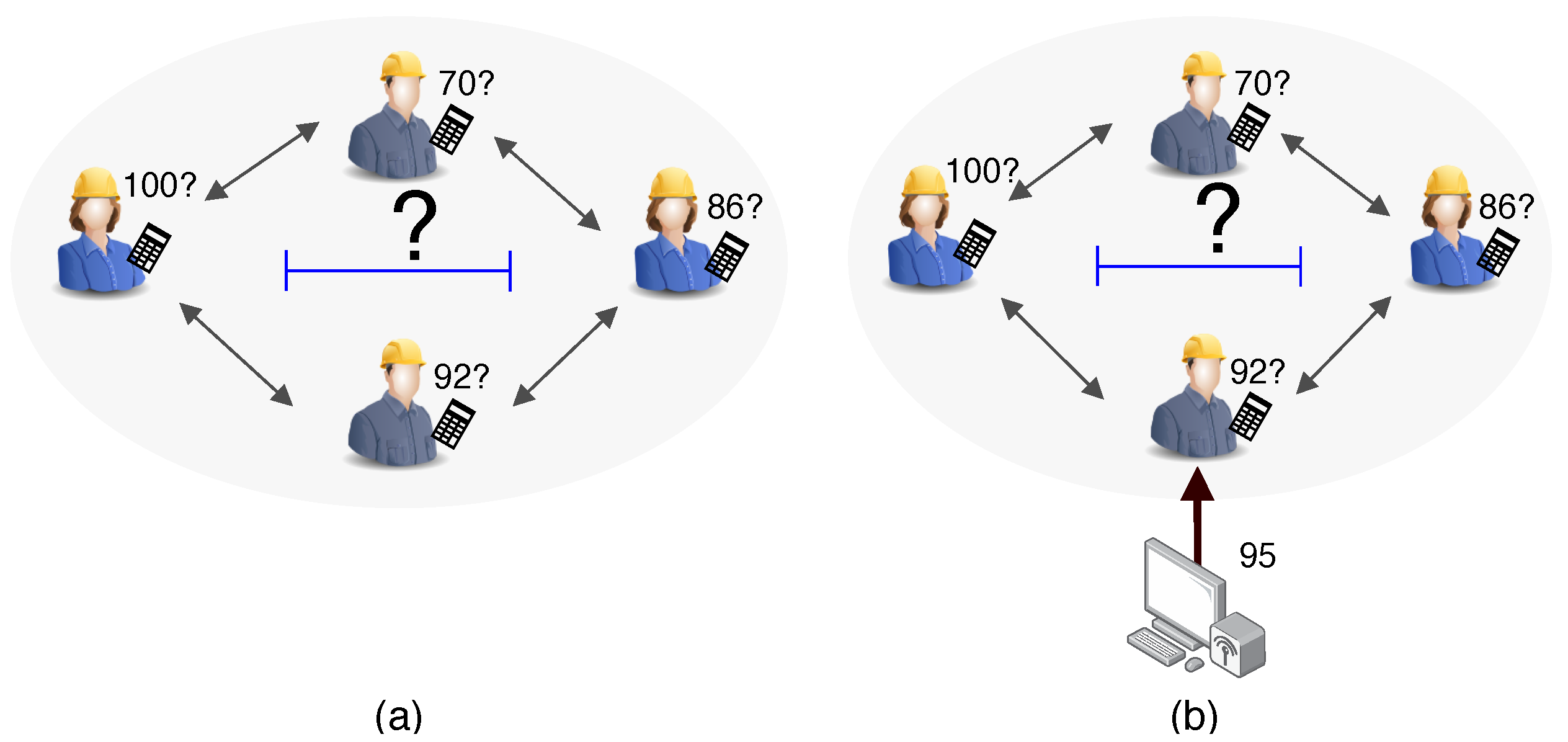
3.2.1. Leaderless Consensus Problem in Continuous-Time

According to DeGroot in 1974, a consensus is achieved in a system just when all elements have converged to the same value [58]. Thus, an agent N i is in consensus with agent N j only if x i ( t ) = x j ( t ) . In other words, the system has a consensus if the following condition is valid for all i and j N * and i j according to (18) [21]
lim t x i ( t ) x j ( t ) = 0 .
The agent’s states x have to be modelled to properly describe the agent’s dynamics [62]. As previously discussed, depending on the system studied the agent’s states may assume a first-, second- or a higher-order to model theirs dynamics [25]. Considering that the state’s dynamic is a linear system described by a first-order integrator model, as assumed in this paper, the control input of the node u i ( t ) , i, is related to its local state at a certain time as
x ˙ i = u i ( t ) , for i N * .
To achieve consensus, a simple protocol may be applied in the system modelled by the graph theory, considering instantaneous information exchanged among neighbours (without communication delay) and fixed topology, according to
u i ( t ) = j = 1 n a i j x i ( t ) x j ( t ) ,
where n is the total number of agents in the system represented by the nodes N i and N j in the graph, a i j is an element in the adjacency matrix A , which models the information flow among vertices. The local states of the agents i and j are represented by x i and x j respectively, for i and j N * . Note that (19) is rewritten in (20)
u i ( t ) = ( j = 1 n a i j x i ( t ) j = 1 n a i j x j ( t ) ) .
In matrix notation, the relation above is the same as shown in (21):
u ( t ) = ( D A ) x ( t ) = L x ( t ) ,
where L is the Laplacian matrix defined in (3) and x R n is the vector related to the states of the agents x ( t ) = [ x i ( t ) , x j ( t ) , x n ( t ) ] .
According to [39], the stability of the system is achieved when the states are described as x ( t ) = [ α , , α ] , for α R , where all nodes are in consensus.
Considering a system modelled by an undirected graph, in which the sum of all states of the agents i does not vary over time, that is, i = 1 n x i ( t ) = 0 , thus the consensus is achieved by the average value of all initial states, as in (22). It is also called the average-consensus problem [39]. In this case, the consensus is asymptotically reached for any initial state
α = i = 1 n x i ( 0 ) n .
If the graph is directed and unbalanced, the consensus may be also achieved, but the average is not guaranteed [39].
Although (22) seems simple to solve, in large and complex systems, the achievement of consensus might become not trivial [39]. A condition for the convergence of the protocols equated in (19) and (21) is presented in Theorem 1.
Theorem 1.
In a multi-agent system, the consensus is achieved if the related graph G is strongly connected. Besides that, the related Laplacian matrix L has null eigenvalue, while the real part of the other eigenvalues is always positive [63].

3.2.2. Leader-Following Consensus Problem in Continuous-Time

The leaderless consensus problem leads to the system convergence to a value related to the agent’s initial states. However, in some practical applications, it is also interesting to make the group of agents converge to a specific and desired value, as an established set point. In this case, the convergence does not depend on the initial states, but on the value introduced into the system as an external signal [63]. Still considering the graph theory, this convergence is possible applying the aforementioned concept of leader-following multi-agent systems (Section 2.1), in which a leader agent, represented by the root node of the graph, establishes a global goal to be reached by all agents in the systems (i.e., the followers), as modelled in Figure 8 and formulated in (23)
u i ( t ) = j = 1 n a i j x j ( t ) x i ( t ) + b i x ref ( t ) x i ( t ) ,
where b i G B represents the nodes that receive the information directly from the leader node, and x ref is the external signal reference to be tracked by the system:
b i = 1 if i G B , = 0 if i G B .
In matrix notation, (23) is rewritten as
u ( t ) = L x ( t ) + B ( x ref ( t ) x ( t ) ) ,
where B = diag ( b i i ) R n × n is a diagonal matrix with entries b i [ 0 , 1 ] according to (24), and x ref R n is the vector with the desired value to be achieved in the system. Considering the example represented by the graph in Figure 8, in which the agent N 4 receives the information directly from the leader, the matrix B is given in (26). The consensus in this case is reached according to Theorem 2:
B = 0 0 0 0 0 0 0 0 0 0 0 0 0 0 0 1 .
Theorem 2.
In a multi-agent system with a leader node, the convergence to the value x ref is reached if the graph is strongly connected including the root node, the leader, independently of the initial states of the followers [64].

3.2.3. Leaderless Consensus Problem in Discrete-Time

Considering the consensus protocol equated in (19) for continuous-time, it may also be defined for discrete-time as [39,65]
x i ( k + 1 ) = x i ( k ) + ϵ j = 1 n a i j ( x j ( k ) x i ( k ) ) ,
which is rewritten in matrix notation as
x ( k + 1 ) = P x ( k ) .
such that k stands for the current iteration. According to [39], the condition expressed in (29) is necessary for the convergence, based on Theorem 3
0 < ϵ < 1 / Δ D ,
where Δ D is the maximum degree of the related Laplacian, Δ D = m a x ( D ) .
Theorem 3.
Considering a system modelled by the undirected graph G , the system reaches a consensus with the application of the protocol in (27) or (28), if the condition described in (29) is considered, independently on the initial states involved [39].

3.2.4. Leader-Following Consensus Problem in Discrete Time

The consensus protocol in discrete-time might also be applied to the system of Figure 8, which represents the leader-following system, as given in (30)
x i ( k + 1 ) = x i ( k ) + ϵ ( j = 1 n a i j ( x j ( k ) x i ( k ) ) + + b i ( x ref ( k ) x i ( k ) ) ) ,
or in matrix notation as
x ( k + 1 ) = P x ( k ) + ϵ B ( x ref ( k ) x ( k ) ) ,
where
0 < ϵ < 1 / Δ D + B ,
for Δ D + B = m a x ( D + B ) .
The convergence is achieved if Theorem 4 is satisfied.
Theorem 4.
In a multi-agent system with a leader node in discrete-time, the convergence to the value x ref is reached if the graph is strongly connected including the root node, i.e., the leader [63], as long as the condition described in (32) is considered, independently on the initial states involved.

3.3. Mathematical Proof

In this section, the steady-state and stability analysis are developed and discussed in detail for the consensus problems presented in Section 3.2, extending also to the directed graphs.

3.3.1. Review for the Analysis in Continuous-Time

To proceed with the stability analysis for the continuous-time formulation, the evaluation is carried out in the sense of Lyapunov theory [66], i.e., the analysis is based on finding the scalar function that verifies the conditions according to Theorems 4.1 and 4.2 in [67].
Consider that V ( x ) is the Lyapunov function candidate and x is the equilibrium point of interest. There are basically three conditions to be verified: the (i) first condition is that V ( x ) has to be continuously differentiable; (ii) the second condition is that V ( x ) = 0 , V ( x ) > 0 in D \ { x } , where D is a regional domain in state space containing the equilibrium and, finally, (iii) the third condition is V ˙ ( x ) 0 D \ { x } .
The stability analysis considers the point x ˜ = x x . The Lyapunov function candidate V ( x ˜ ) chosen for the stability analysis is given in (33) and the related gradient in (34)
V ( x ˜ ) = 1 2 x ˜ x ˜ ,
V ( x ˜ ) = x ˜ .
It is observed that the first and second conditions of Lyapunov theory are satisfied by the chosen function. Thus, in the following subsections, the stability analysis is focused on the verification of the third condition as follows:
V ˙ = V ( x ˜ ) x ˜ ˙ 0 .
To generalise the consensus problem formulations for the different graphs, this condition is analysed based on the Laplacian properties previously discussed in Section 2.2.1.

3.3.2. Leaderless Consensus Problem in Continuous-Time

  • Steady-State Analysis: to analyse the steady-state, the focus is on the equilibrium point x ˙ = 0
    x ˙ = L x .
    Due to the first property of the Laplacian ( L 1 = 0 ) presented in (8), which holds for the three graph topologies covered herein, there is just a specific value of α in which the equilibrium is achieved [39], as expressed in (36) and (37)
    0 = L x = L α 1 ,
    x = ( α , α , , α ) .
    To define the value of α achieved in the convergence, let us consider the second Laplacian property discussed in Table 1
    X ˙ = γ L x = 0 ,
    which means that γ x is an invariant quantity [39], in which the sum of the states at any time t has to be the same. Thus, as the initial states ( t = 0 ) are known, the equilibrium x = ( α 1 ) is found:
    γ x = γ ( α 1 ) = α γ 1 = γ x ( 0 ) , α = γ x ( 0 ) γ 1 .
    Considering γ 1 = i = 1 n γ i ,
    α = γ x ( 0 ) i = 1 n γ i = i = 1 n γ i x i i = 1 n γ i .
    As summarised in Table 1, for undirected and direct balanced graphs, γ is an unitary vector since the sum of the columns elements of L is also 0. It leads to i = 1 n γ i = i = 1 n 1 i = n [39] and then
    α = 1 x ( 0 ) n = i = 1 n x i ( 0 ) n ,
    which is the average of the agents’ initial states, as presented in (22).
    Note that, as expected, α dir / unb is not the average as the other cases, but a kind of weighted average value related to the left eigenvector, associated with the trivial eigenvalue.
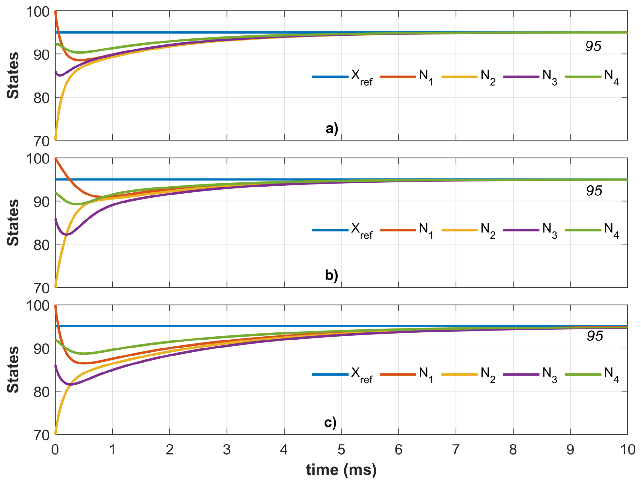
  • Stability Analysis: omitting t for the sake of simplicity, the consensus problem in (21) is rewritten in terms of x ˜ in (41)
    x ˜ ˙ = L x ˜ .
    Replacing x ˜ ˙ in (35) by (41) and V ( x ˜ ) by (34), it results in
    V ˙ = V ( x ˜ ) ( L x ˜ ) 0 = x ˜ L x ˜ 0 .
    Since (42) is quadratic and multiplied by negative sign, it complies with the third condition of the Lyapunov analysis if and only if L is positive semi-definite, as shown in Table 1. Under this condition, it is ensured that the real part of eigenvalues in L are non-positive for all x ˜ , as desired. Due to the third property of Table 1, the stability is directly guaranteed for undirected and directed balanced graphs. However, for directed unbalanced graphs, this property has to be checked case by case, since it is not possible to generalise the positive semi-definiteness without knowing the system. As previously checked for the examples considered in Figure 7, all Laplacian matrices are positive semi-definite. Hence, according to Lyapunov theory, the three different topologies may be considered globally asymptotically stable.

3.3.3. Leader-Following Consensus Problem in Continuous-Time

  • Steady-State Analysis: let us consider now (43)
    L x + B x = B x ref .
    From the second Laplacian property ( γ L x = 0 ), (43) is multiplied by the Laplacian left eigenvector:
    γ L x + γ B x = γ B x ref , 0 + γ B x = γ B x ref .
    For the sake of simplicity, let us consider that there is just one agent receiving the information directly from the leader, as in the example given in Figure 8. This means that just one term in the diagonal of the matrix B is equal to one and the other elements are equal to zero, as in (26). Then, for undirected and directed graphs,
    B x = B x ref .
    Replacing then (44) in (43),
    L x + B x ref = B x ref , L x = 0 ,
    which, due to the first Laplacian property ( L 1 = 0 ), leads to the same analysis as in (36) and (37). It shows that, to ensure (45), all states have to achieve the same value. If the agent associated with b i i = 1 is equal to the value dictated by the leader node, all agents therefore have achieved the same value
    x = x ref .
  • Stability Analysis: analogously to the analysis performed in Section 3.3.2, (25) is rewritten as per (46)
    x ˙ = L x + B ( x ref x ) .
    Considering the point of interest as x ˙ = 0 ,
    0 = L x + B ( x ref x ) .
    For the stability analysis, consider the operating point at x ˜ = x x * obtained by subtracting (47) of (46)
    x ˜ ˙ = L x ˜ + B x ˜ .
    Applying the same Lyapunov function of (33), the first conditions for stability in the Lyapunov theory still hold. Thus, it is necessary to verify the expression in (35). Applying (48) and (34) in (35), one obtains:
    V ˙ = x ˜ ( L + B ) x ˜ 0 .
    Similarly to the analysis conducted for the leaderless consensus, the stability depends on the sign definiteness of the sum L + B . It is known that the sum of positive semi-definite matrices is a positive semi-definite matrix. B is the diagonal matrix with ones and zeros; then, B is positive semi-definite. Therefore, to guarantee V ˙ 0 , it is necessary to ensure that L is also positive semi-definite, which leads to the same conditions already discussed for undirected, directed balanced and directed unbalanced graphs in the previous sections. Additionally, according to [68], since the row sums of the resulting matrix L + B are no longer always zero, the trivial eigenvalue is no longer at zero. The eigenvalues of the related matrix are all greater than zero, which makes the resulting matrix not just positive semi-definite, but positive definite [68]. The formulations presented in continuous-time are summarised in Table 3.

3.3.4. Review for the Analysis in Discrete-Time

To carry out this evaluation, two important tools are covered herein–Gershgorin Circle Theorem [51,52,69,70] and Perron–Frobenius Theorem [70,71]—which are intertwined concepts to evaluate the spectral radius of a matrix, informing the boundary of the eigenvalues, even without knowing each one of them [72].
Combining the properties of both theorems, the stability in discrete-time is analysed based on the conditions described in the following, according to [39].
Theorem 5.
For a system x k + 1 = M x k , and λ i being its eigenvalues, the stability is guaranteed if the eigenvalues of M lie inside the unit circle of the Gershgorin disks and if the Perron–Frobenius Theorem was attained.
The proof of Theorem 5 is done by analysing whether the matrix M is irreducible (graph strongly connected), non-negative ( m i j 0 ), primitive (a single λ i with maximum modulus) and row-stochastic (maximum | λ i | = 1, i.e., inside the unit circle).

3.3.5. Leaderless Consensus Problem in Discrete-Time

  • Steady-State Analysis: to analyse the steady-state conditions, it is considered that
    x k + 1 x k = ϵ L x k , 0 = ϵ L x k .
    Since ϵ is a positive scalar, the analysis is performed based on the properties of L , as previously discussed in (36) and (37). The value of convergence α assumes the same relations presented in (40) for undirected and directed balanced graphs and (39) for the directed unbalanced graph.
  • Stability Analysis: let us consider once more the consensus problem equated in (41), and that x ˜ ˙ is approximated by (49)
    x ˜ ˙ = d x ˜ d t x ˜ k + 1 x ˜ k Δ t x ˜ k + 1 x ˜ k ϵ ,
    where x ˜ k + 1 and x ˜ k are the state x ˜ at the iteration k + 1 and k , respectively, and Δ t = ϵ is called step-size. Since
    ϵ > 0 ,
    one can rewrite (41) based on (49) and obtain
    x ˜ k + 1 x ˜ k = ϵ L x ˜ k , x ˜ k + 1 = ( I ϵ L ) x ˜ k .
    where I ϵ L = P [48].
    To verify the stability according to Theorem 5, the properties summarized in Table 2 are here recalled and verified. To satisfy the Perron–Frobenius Theorem, P has to be irreducible, non-negative and primitive. The Perron matrices of all graph topologies covered in this paper are irreducible, since all of them are strongly connected. To ensure that P is also non-negative, the value ϵ has to be bounded, as indicated in (50)
    P 0 , I ϵ D + ϵ A 0 .
    The matrix A has non-negative entries, independently of the graph topology, and, consequently, since ϵ > 0 , ϵ A is also a matrix with non-negative entries. Thus, the analysis is focused on the other terms of (50), as
    I ϵ D 0 .
    To guarantee the second condition of Table 2, analysing element by element, it is necessary to consider the worst case condition of matrix D , its maximum value, as shown in:
    1 ϵ d i i 0 , ϵ 1 m a x ( d i i ) .
    Thus, the step-size condition to make the Perron matrix non-negative in (53) is defined such that m a x ( D ) = Δ D
    0 < ϵ 1 Δ D .
    Observe that the maximum step-sizes for the Laplacian and Perron matrices in (5)–(7) are: ϵ L und = 1 / 2 , ϵ L dir / bal = 1 , ϵ L dir / unb = 1 / 2 , which means that the value ϵ = 0.4 chosen to calculate the Perron matrices satisfies (53) for all topologies covered herein. Consequently, the Perron matrices obtained have all entries greater than zero. Just to exemplify, if ϵ = 0.6 > 1 / Δ D und is chosen for the undirected graph, the Perron matrix is no longer non-negative.
    Proceeding with Theorem 5, it is also necessary to ensure that P is primitive (by checking if P n 2 2 n + 2 has only positive entries [73]). For the sake of simplicity, let us consider the undirected graph, with ϵ = 0.4 and the condition P n 2 2 n + 2 being attained.
    To show the relation of the property with the eigenvalues, the result obtained through Matlab is λ = { 1.0 , 0.6 , 0 , 0 } . Observe that, as expected, the eigenvalue with maximum modulus appears just once. However, whether it is chosen ϵ = 0.5 , exactly at the upper limit of (53), P n 2 2 n + 2 has no longer only positive entries, but also zeros. Consequently, the eigenvalues obtained are λ = { 1.0 , 0 , 0 , 1 } , and they do not satisfy the condition of the algebraic multiplicity equal to one for the maximum eigenvalue modulus (a single eigenvalue with maximum modulus). For this reason, the value of ϵ has to be bounded according to (54)
    0 < ϵ < 1 Δ D .
    Besides the properties already analysed, it is also necessary to ensure that the maximum modulus of the eigenvalues is equal to one, in order to guarantee that they lie inside the unit Gershgorin circle.
    Note that the fourth property highlighted for the Perron matrix, P 1 = 1 , gives information not only on one of the eigenvalues of the matrix, but also on its spectral radius [73]. According to Table 2, it is a characteristic of all topologies covered herein. Thus, it means that P is row stochastic for all topologies, which implies that the trivial eigenvalue of the matrix is equal to one and, due to the Gershgorin circle, this is also the value of the spectral radius of the matrix. Going back to Perron–Frobenius Theorem, since the other conditions for this Theorem are already satisfied, it is known that all other eigenvalues have a smaller modulus than one.
    Finally, according to Theorem 5, all graph topologies covered in this paper are then stable in discrete-time as well as in continuous-time.

3.3.6. Leader-Following Consensus Problem in Discrete-Time

  • Steady-State Analysis: for the steady-state analysis and the value of convergence, the relations in (55) are considered
    x k + 1 x k = ϵ L x k ϵ B x k + ϵ B x ref , 0 = ϵ L x k ϵ B x k + ϵ B x ref , ϵ L x k + ϵ B x k = ϵ B x ref , L x k + B x k = B x ref .
    Note that the relation in (55) is the same as in (43). Then, the analysis is the same as performed for continuous-time.
  • Stability Analysis: for the leader-following consensus problem in discrete-time considering the relation in (48), which is rewritten in discrete-time based on the approximation in (49), the following is obtained:
    x ˜ k + 1 x ˜ k = ϵ L x ˜ k ϵ B x ˜ k , x ˜ k + 1 = ( I ϵ L ϵ B ) x ˜ k , x ˜ k + 1 = ( P ϵ B ) x ˜ k ,
    where ( P ϵ B ) = Q and Q R n × n . All the properties analysed for the leaderless consensus still hold for P in (56). Considering that B is a diagonal matrix with ones and zeros, the effect of the term ϵ B on the eigenvalues of Q must be analysed. The expression (56) is rewritten as
    x ˜ k + 1 = ( I ϵ ( L + B ) + ϵ A ) x ˜ k .
    Considering (57), an increase in the degree of matrix Q is observed, through the beta term B, according to the number of agents that receive information from the leader. Thus, the output matrix Q does not loose connectivity in comparison with the leaderless formulation, remaining still related to a strongly connected graph and, therefore, it is still irreducible.
    To ensure that Q is non-negative and primitive, analogously to the analysis carried out for the leaderless consensus problem in (51)–(53), the maximum value of the step-size is:
    1 ϵ ( d i i + b i i ) > 0 , ϵ < 1 m a x ( d i i + b i i ) ,
    which leads to
    0 < ϵ < 1 Δ D + B ,
    This is the same condition presented by [74] in different approaches for the purpose of stability analysis.
    The features analysed until now ensure that the properties of the Perron–Frobenius Theorem hold for the matrix Q . Now, it is necessary to evaluate if the new eigenvalues still lie inside the unit Gershgorin circle.
    Differently from the leaderless consensus, the fourth property of the Perron matrix is no longer valid for all rows in the matrix Q . However, due to the bounded value of ϵ , the Q is affected just on its diagonal. According to Gershgorin Theorem, this means that the term ϵ B changes the centre of the Gershgorin disks related to Q , keeping the same radius of P . For the example considered in Figure 8, the eigenvalues obtained in Matlab reinforce the features discussed λ = { 0.3029 , 0.2588 , 0.4000 , 0.9441 } . Observe that the maximum modulus of the related eigenvalues is less than one.
    Due to the features presented to ensure that the eigenvalues of the system are also within the unit circle, the leader-following consensus is also stable in discrete-time for all graph topologies. Different approaches for the stability analysis of leader-following consensus in discrete-time are found in [75,76]. The analysis presented for leader-following and leaderless consensus in discrete-time is summarised in Table 4.
The leaderless and leader-following formulation in discrete-time is applied to the three graph topologies of Figure 7. For the leader-following problem, let us consider the graph of the Figure 8 as base, for the different communication NTs shown in Figure 7. The Laplacian matrices for each graph topology are given in (5)–(7), and the matrix B for the leader-following problem in (26). As previously discussed, the steady-state is achieved when all agents have the same value α . The convergence results obtained are shown in Figure 9 and Figure 10, respectively. For the leaderless consensus, the value depends on the agent’s initial states, as expected. For the unbalanced case, the system does not converge to the average, but to the value obtained through a weighted average based on its left eigenvector γ . For the leader-following case in all different communications covered herein, however, the system converges to the reference value independent on the states’ initial values.

4. Application to Microgrid Control

This section presents an overview on the application of consensus protocols in the field of MG control in recent years, which has been applied either in DC (e.g., [77]), AC systems (e.g., [78]) or even in hybrid AC/DC MGs (e.g., [79]).

4.1. Features of the Microgrid

The MGs are multi-agent systems which may be also modelled by the graph theory presented in Section 2.1 (e.g., [80,81]). In a consensus protocol applied in a multi-agent system, the state value of each vertex is related to physical quantities in the system [82]. It is well known that an MG represents a very diversified system, such as the diversity of electrical elements integrated in this kind of structure, which may present linear and nonlinear behaviours, considerably affecting the electrical quantities involved. Since the consensus protocols have to be designed considering these particularities, in the applications in MG control presented in [83,84,85,86], the controlled quantities in the system are described by nonlinear and/or with high-order dynamics. Besides that, since the plug and play capability of DGs is an important feature for an MG, the topology of the system might change over time. Thus, time-varying topologies in MG applications are extensively explored in [36,87,88]. With higher or lower impact, the imperfections of communication-based applications might also not be neglected, especially on the secondary level in the control organisation [89]. This is the reason that justifies the increasing number of studies dedicated to exploring the impact of time-delays in MGs, where some examples are found in [19,36,68,90,91,92].

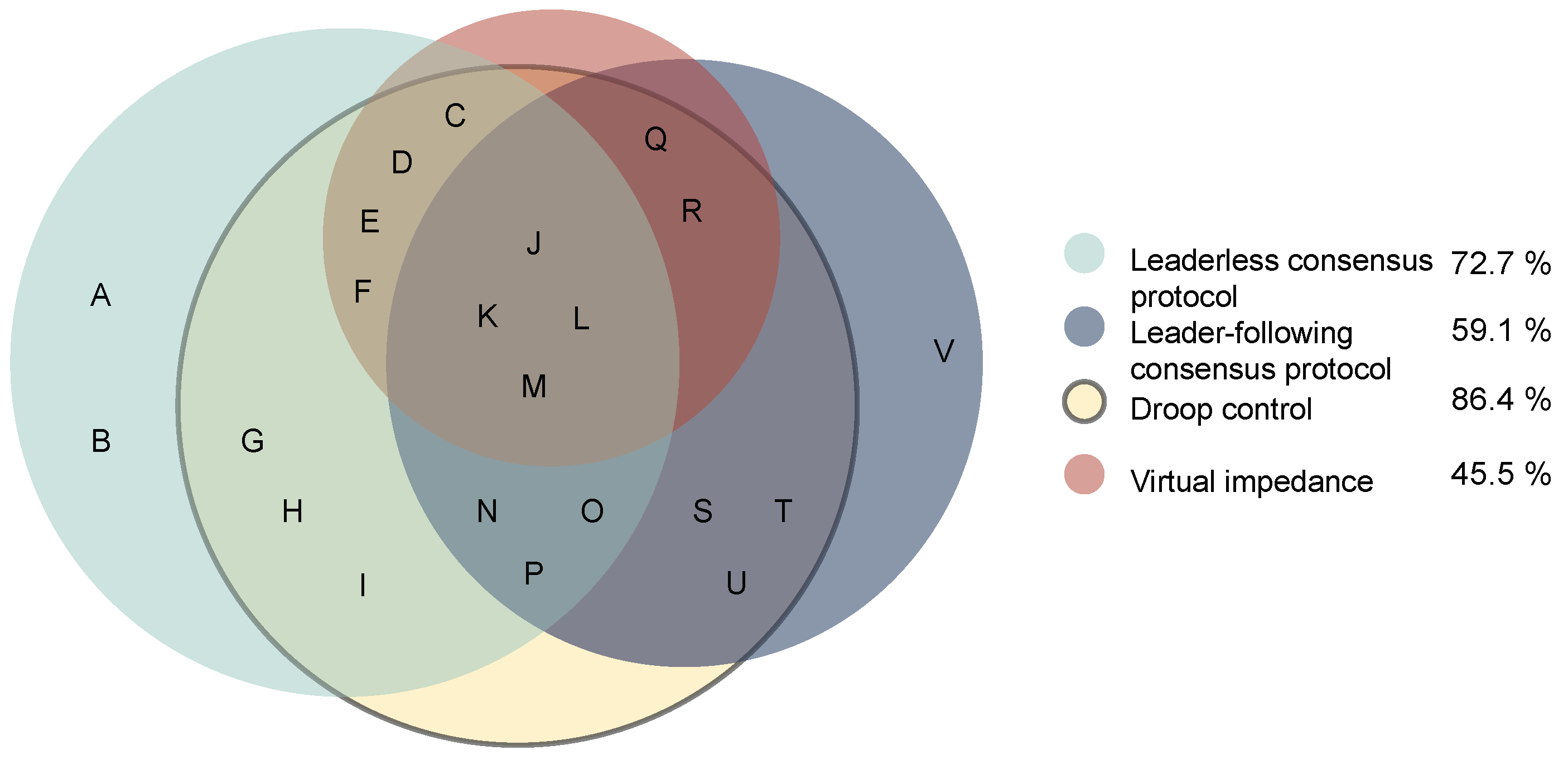
4.2. Contributions from the Literature

For many years, the droop control has been pointed out as the most common method for power sharing among DGs [93] in a fully decentralised manner and in recent years, as evidenced in Figure 11, it has been combined with the consensus protocols [17] as in the following works from the same sample considered in Section 1: [59,63,84,94,95,96,97,98,99,100,101,102,103,104,105]. Regarding the control configurations of the cited works, a hierarchical organisation of the control attributions is commonly used, and the consensus protocol is often dedicated to the secondary control in order to deal with the trade-off between power sharing and voltage and frequency regulation inherent in the droop control technique. Few of the works from this sample explore the consensus-based control strategy without linking it to the droop control technique, as carried out in [78,106,107]. Within these combinations, as indicated in Figure 11, the association of the droop control with consensus protocols represents almost 90 % of the analysed proposals.
Regarding the scope of these studies, it is observed that almost all of them focus on the internal coordination of the MG’s elements and few are dedicated to studying the connection of different MGs (i.e., the MG clusters), as the recent work in [108], out of the samples considered. With few exceptions, the studies use only radial topology to validate their proposals, and the meshed topologies are generally not considered and not even discussed. In addition, the focus is usually the islanded operation of the MGs. Few studies deal with both operational modes and the transition between them. The power dispatchability is rarely addressed.
The consensus technique is a flexible method for the control system development in MG applications, considering several different characteristics involved in such systems. The problem given in the introduction may be solved by different variations of the consensus protocols. The intention herein, however, is not to focus on a specific consensus-based control strategy but provide a general overview of different approaches found in the literature, which apply the consensus theory in the MG control. For this purpose, Figure 12 and Figure 13 present the main characteristics of the selected publications, keeping the same four selected features to characterize the control systems, i.e., the control configuration, control architecture, communication infrastructure and control strategy. Regarding the scope and control application of those proposals, it is observed that almost all of them focus on the internal coordination of either AC MG or DC MG. Few works are dedicated to studying Hybrid Microgrid (HMG), both AC and DC sides and the power sharing among them through interlink converters. Examples of this last small group are found in recent publications, such as [79,109]. The work of [110] goes a step further, exploring also the connection of different MG (i.e., the MGC).
Figure 11. Sample of publications related to consensus protocol in control systems for microgrid control strategies and techniques combined. Legend: A—Duan, 2019 [78], B—Pham, 2021 [111], C—Zhou, 2019 [94], D—Yoo, 2020 [79], E—Burgos, 2020a [112], F—Xu, 2021 [113], G—Schiffer, 2016 [84], H—Fuad, 2017 [59], I—Zhou, 2019 [114], J—Simpson, 2015 [83], K—Yu, 2018 [63], L—Keshavarz, 2021 [115], M—Wei, 2017 [116], N—Burgos, 2020b [117], O—Hou, 2018 [118], P—Vergara, 2019 [100], Q—Espina, 2021 [109], R—Zhou, 2020 [110], S—Chen, 2019 [99], T—Ullah, 2021 [119], U—Tao, 2020 [120], V—Huang, 2017 [106].
Energies 15 08536 g011
Regarding the control techniques adopted, contributions which use the typical combination of the consensus protocol with droop control have been proposed since the first publications covered in the sample analysed. This high interest may be justified by the wide applicability of this method.
The proposal in [83] applied this technique to solve the trade-off between the conflicting achievements of voltage regulation and reactive power sharing in islanded MG. In [95], a state predictor is inserted into the combination of droop with consensus techniques, in order to improve the convergence time of the consensus protocol. The principle is based on the eigenvalues properties of the Laplacian matrix that describe the connectivity of the system and are related to its convergence. Results better than those obtained without the state predictor are presented. This contributes to reducing the communication and computational requirements, necessary for proper system operation.
In [96], the principles of the consensus protocol are used to develop a secondary control to provide accurate active and reactive power sharing, restoring the desired voltage and frequency levels. The concepts of average consensus protocol and leader-following systems are combined, but called regulator synchronization problem and tracking synchronization problem, respectively. In this work, the joule losses along the distribution lines are considered and the virtual impedance technique is also applied in the primary droop control. An interesting study of system stability is also addressed.
Accurate reactive power sharing and voltage control is also aimed for in [97]. It develops an interesting secondary control strategy based on the combination of consensus-based reactive power control and the so-called containment-based voltage control. This last one is formulated according to the principles of the leader-following systems. Droop control is introduced for reactive power sharing and the consensus leader-following with two leader agents for voltage regulation. This voltage control operates within a limited range, previously defined for each DG. This study presents the complete modeling for small-signals stability study and the control reliability is analysed for different system topologies.
Different from the mentioned two-level control works, in which droop technique normally operates at the primary level and consensus at the secondary level, Ref. [84] proposes a single consensus-based control to regulate the voltage level, focused on the reactive power sharing. Frequency droop control is still applied for active power sharing.
In addition to accurate reactive power sharing, mainly aimed for by most of these works, Ref. [94] also covers unbalance and harmonic compensation at the PCC. Unlike [63] and other works based on static virtual impedance, considering positive or negative sequence, both are considered in [94], as well as the harmonic virtual impedance. They are dynamically regulated by applying the consensus technique, so that it is possible to adjust the virtual impedance at the fundamental frequency and at the specific frequencies of the selected harmonics. The consensus protocol is also used to compensate the voltage deviation caused by the droop control and by the virtual impedance itself. This is achieved by incorporating the effect of the line impedance using information from adjacent DG to estimate the average voltage in the grid and to determine the correction factor.
Despite not including the harmonic compensation in the control proposal, Ref. [63] contributes with a mathematical proof for more complex systems, such as meshed power grids. According to the authors, reactive power can only be accurately shared if there is at least minimal communication among the agents. This study also explores the concept of leader-following systems, used to ensure that DG not only reach a consensus, but can converge to a desired point of operation, following a given reference.
In [99], the same authors of [95] focus on active power sharing under the effect of disturbances in the communication. Droop control is again applied to the local control, and a strategy called pinning-consensus-based control is developed for the secondary control of an MG. The control strategy is based on the concept of leader-following systems. In addition to this control, the study also proposes the introduction of observer states in order to support in the estimation of the communication disturbances. The observer states mitigate the related impacts, maintaining the stability of active power sharing without the need for interrupting the failed communication link.
In [100], in addition to the primary and secondary controls, a tertiary control is also proposed. Droop control is implemented as local control, and the controls based on the primal-dual constrained decomposition and consensus-based control are implemented in the secondary and tertiary levels, respectively. It focuses on an optimal power dispatch considering the generation costs.
The work of [104] provides important contributions to real applications. It takes into account any influence of variable communication delays in the control development, obtaining good results, especially in the system stability analysed by the Lyapunov theory.
In the last two years, important achievements to this combined consensus/droop-based technique were published in the literature. In [112], the conservative power theory is applied to extract the balanced, unbalanced and distorted current and power components. The virtual impedance technique is applied and is dynamically adapted through a consensus-based control to compensate imbalances and harmonics in the system. In this work, frequency and voltage are regulated and active and reactive power are shared proportionally to the DG capacity. A different feature observed in [112] in comparison with most of the publications is the control development in the abc frame, dispensing the need of sequence separation. This avoids effects of noises, sampling time and distortions, which commonly influences separation algorithms [112].
A wider application of consensus/droop-based control is applied in [79,109]. They address HMG. In both proposals, the main goals are the regulation of the main quantities of each AC and DC side and also control the power sharing among them, which are performed by interlink converters. As considered in [79], the line impedances influence not only the reactive power, but also the DC current sharing. In this work, the virtual impedance is designed based on the average value of the DG’ currents, calculated by the LLCP (average-consensus).
In [113], the frequency deviation of traditional droop approaches is reduced by introducing phase angle measurements from synchronous phasor measurement units (PMU) data. The accuracy of voltage and reactive power sharing is achieved by the implementation of observer-based voltage controller with finite-time convergence velocity. Additionally, this proposal also considers the generation operational costs in a cost minimization problem. In [115], voltage and frequency are regulated by the implementation of a consensus-based adaptive control structure, considering the nonlinearities of these kinds of systems.
As is shown in Figure 11, few of the covered publications explore the consensus-based control strategy without linking it to droop control, as carried out in [78,106,107]. In the work of [78], a control strategy is developed based on the consensus-based control and on the power flow analysis, focused on voltage regulation and active power sharing, taking into account the existing natural coupling due to the line impedance. In [106], the LFCP is used for the purpose of coordinating different ESS, in order to provide a reduction of power oscillations at the PCC.
Regarding the methods and proposals evaluation, a complement of Figure 12 and Figure 13 is presented in Figure 14 and Figure 15, respectively.
Concerning the features of the control systems, as the islanded operation mode usually receives more attention, normally the converters operate in voltage-controlling mode. As discussed previously, the hierarchical architecture is widely applied, making the combination of different techniques in the same system possible.
Within these combinations, as indicated in Figure 11, the association of the droop control and consensus-based control represents more than 80% of the analysed proposals, which normally means also that the voltage magnitude and system frequency are the controlled quantities. Many of these studies have used the principle of leader-following systems, applying external references to the control, making all agents converge to a predefined or calculated value at some level in the control hierarchy.
Since only a few studies cover the connected operation mode, the regulation of the power flow at the point of common coupling is normally not approached. Different topologies are used, requiring communication only among adjacent DGs—usually bidirectional. The results are obtained mostly by simulations, commonly developed in Matlab/Simulink. Approximately 15% of the sample use experimental implementations to validate the strategies. These results are fully presented and discussed through graphs covering the profile of the quantities of interest (such as voltage, frequency, active power and reactive power) and in some cases with stability analysis. No study applying a specific methodology for analysis and comparison with other strategies, such as using performance, figure of merit, and quality indicators, is identified.
Figure 16 presents the main subjects discussed in the publications analysed in detail. An expressive concentration of efforts towards some common objectives is observed, such as: accuracy in the active and reactive power sharing, and voltage and frequency regulation still being the main topic of interest in most of the works.
The summary presented in Figure 17 is based on the parameters adopted and presented below in the diagram. The numbers within brackets are features observed in the related publication. The colors were used to highlight these selected features as follows: red is high, yellow is medium and green is low. The criteria adopted to categorize each piece of research were:
  • if the system has at least two of the enumerated elements, the control is considered of high complexity; medium if one element is present, and low if none of the listed characteristics are observed;
  • limitations regarding the reliability: the classification high is when the proposal does not present any tolerance or alternatives to deal with the conditions (1) and (2) or if the proposal depends on a specific agent or MC; medium if the strategy deals with the condition (1) or (2) or/and (3), and low if the control is able to deal with all scenarios considered and is not dependent on a leader or MC;
  • the limitation to choose the communication NT is considered high in case of scenarios (1) or (2), medium if (3) and low for scenarios (4) or (5);
  • the limitation for the project applicability is measured based on the diversity of elements from real applications considered in the simulations, so that the proposal is considered highly limited if only one or two of these elements are considered, medium if at least three are addressed, and low if more than three are considered in the scenarios or systems chosen. If the stability is not discussed in any scenario, the limitation is classified as high because the strategy may not be generalized.

4.3. Benefits and Challenges

The application of the consensus protocol offers interesting benefits. However, as in any other control strategy, there are still some associated challenges. The benefits of this technique normally represent an intermediate solution in comparison to the ones achieved with fully centralised or decentralised structures. The most important benefits are listed in the following, as well as the related challenges which still require attention.

4.3.1. Benefits

  • Simplicity in the structure [36];
  • High redundancy [36];
  • High scalability [36];
  • Independence of a master controller, although it could also be applied, if desired;
  • Resilience in fault conditions due to the sharing of the attributions among the agents [25];
  • Shorter communication NT in comparison with centralised structures;
  • Deep development and maturity of the consensus technique in other areas of knowledge;
  • Possibility to be applied at different control levels within the hierarchical configuration;
  • Possibility to be combined with different control strategies;
  • Flexibility to define the variable of interest (agent’s states).

4.3.2. Challenges

  • Need of communication NT compared with fully decentralised structures [36];
  • Influence of communication delays [36];
  • Influence of topology changes [25].
Although the consensus protocol may be influenced by communication delays and topology variation, and these challenges still deserve attention in this segment, there are already important contributions in the literature dealing with these issues, as already presented, especially in other areas of knowledge.
For [12], the control system in an MG must overcome three major challenges: (i) communication limitations, hl(ii) topology variations due to the connection and disconnection of DGs and failures, and (iii) low inertia and stability of the systems involved.
In [36,99], the communication delay, an inherent feature in cooperative multi-agent systems, is one of the major development demands for MG applications. Furthermore, the authors consider that solutions to mitigate the influence of MG topology variations still deserve attention. They need to be developed for better coordination of these systems, as this is also an inevitable feature that tends to become even more significant with the scalability and modularity of the MGs. A third need mentioned by [36] concerns the coordination of different MGs, as MG clusters, using the multi-agent systems approach, where not only are the internal characteristics of the MG considered, but also the interactions among different MGs.
In general, the compromise of different priorities with a single and simple technique may be considered as an important challenge. Each priority in an MG project leads to specific needs and consequently to specific challenges.

5. Conclusions

In this paper, an overview of the fundamentals of the consensus protocol technique was presented as a start guide for application in the control system of microgrids. The context in which the consensus protocol emerged over the years was discussed and the concepts of multi-agent systems and graph theory for system modelling were reviewed. The protocol formulation was presented, including detailed steady-state and stability analysis for strongly connected undirected and directed graphs, in both continuous- and discrete-time.
Some contributions in the field of microgrids were discussed, and their main features were categorised, making the identification of some trends for new studies possible.
Although the consensus protocol has been developed for many years in other areas of knowledge, there are still important challenges which deserve attention in the applications in control systems of microgrids, such as the power sharing accuracy and voltage/frequency regulation, stability conditions, complexities of the system dynamic, development of a tertiary control which allows the achievement of macro objectives, impact of communication failures and time-delays and the plug and play process of DGs. However, the flexibility offered by the technique makes its combination with different control strategies possible in order to overcome or minimise the aforementioned challenges, thus opening a wide range of possibilities to be explored in this segment.

Author Contributions

D.F. and S.S. contributed equally to the conceptualization, D.F., S.S., D.B., G.B. and E.T. contributed equally to the methodology, W.S. contributed to the writing draft preparation, review and editing. All authors have read and agreed to the published version of the manuscript.

Funding

This research received no external funding.

Data Availability Statement

Not applicable.

Conflicts of Interest

The authors declare no conflict of interest.

References

  1. Adefarati, T.; Bansal, R.C. Integration of renewable distributed generators into the distribution system: A review. IET Renew. Power Gener. 2016, 10, 873–884. [Google Scholar] [CrossRef]
  2. Hooshyar, A.; Iravani, R. Microgrid Protection. Proc. IEEE 2017, 105, 1332–1353. [Google Scholar] [CrossRef]
  3. Zeng, Z.; Li, X.; Shao, W. Multi-functional grid-connected inverter: Upgrading distributed generator with ancillary services. IET Renew. Power Gener. 2018, 12, 797–805. [Google Scholar] [CrossRef]
  4. Bullich Massagué, E.; Díaz González, F.; Aragüés Peñalba, M.; Girbau-Llistuella, F.; Olivella Rosell, P.; Sumper, A. Microgrid clustering architectures. Appl. Energy 2018, 212, 340–361. [Google Scholar] [CrossRef]
  5. Hirsch, A.; Parag, Y.; Guerrero, J. Microgrids: A review of technologies, key drivers, and outstanding issues. Renew. Sustain. Energy Rev. 2018, 90, 402–411. [Google Scholar] [CrossRef]
  6. Madureira, A.G.; Pecas Lopes, J.A. Coordinated voltage support in distribution networks with distributed generation and microgrids. IET Renew. Power Gener. 2009, 3, 439. [Google Scholar] [CrossRef] [Green Version]
  7. Bevrani, H.; Ghosh, A.; Ledwich, G. Renewable energy sources and frequency regulation: Survey and new perspectives. IET Renew. Power Gener. 2010, 4, 438. [Google Scholar] [CrossRef] [Green Version]
  8. Lasseter, B. Microgrids [distributed power generation]. In Proceedings of the 2001 IEEE Power Engineering Society Winter Meeting, Conference Proceedings (Cat. No.01CH37194). Columbus, OH, USA, 28 January–1 February 2001; Volume 1, pp. 146–149. [Google Scholar]
  9. Olivares, D.E.; MehriziSani, A.; Etemadi, A.H.; Canizares, C.A.; Iravani, R.; Kazerani, M.; Hajimiragha, A.H.; Gomis-Bellmunt, O.; Saeedifard, M.; Palma-Behnke, R.; et al. Trends in Microgrid Control. IEEE Trans. Smart Grid 2014, 5, 1905–1919. [Google Scholar] [CrossRef]
  10. Rocabert, J.; Luna, A.; Blaabjerg, F.; Rodríguez, P. Control of Power Converters in AC Microgrids. IEEE Trans. Power Electron. 2012, 27, 4734–4749. [Google Scholar] [CrossRef]
  11. Han, Y.; Li, H.; Shen, P.; Coelho, E.A.A.; Guerrero, J.M. Review of Active and Reactive Power Sharing Strategies in Hierarchical Controlled Microgrids. IEEE Trans. Power Electron. 2017, 32, 2427–2451. [Google Scholar] [CrossRef]
  12. Yazdanian, M.; Mehrizi-Sani, A. Distributed Control Techniques in Microgrids. IEEE Trans. Smart Grid 2014, 5, 2901–2909. [Google Scholar] [CrossRef]
  13. Fagarasan, I.; Stamatescu, I.; Arghira, N.; Hossu, D.; Hossu, A.; Iliescu, S.S. Control Techniques and Strategies for Microgrids: Towards an Intelligent Control. In Proceedings of the 2017 21st International Conference on Control Systems and Computer Science (CSCS), Bucharest, Romania, 29–31 May 2017; pp. 630–635. [Google Scholar]
  14. Kaviri, S.M.; Pahlevani, M.; Jain, P.; Bakhshai, A. A review of AC microgrid control methods. In Proceedings of the 2017 IEEE 8th International Symposium on Power Electronics for Distributed Generation Systems (PEDG), Florianópolis, Brazil, 17–20 April 2017; pp. 1–8. [Google Scholar]
  15. Morstyn, T.; Hredzak, B.; Agelidis, V.G. Control Strategies for Microgrids with Distributed Energy Storage Systems: An Overview. IEEE Trans. Smart Grid 2018, 9, 3652–3666. [Google Scholar] [CrossRef] [Green Version]
  16. Bracale, A.; Angelino, R.; Carpinelli, G.; Mangoni, M.; Proto, D. Dispersed generation units providing system ancillary services in distribution networks by a centralised control. IET Renew. Power Gener. 2011, 5, 311. [Google Scholar] [CrossRef]
  17. Li, Y.W.; Kao, C.-N. An Accurate Power Control Strategy for Power-Electronics-Interfaced Distributed Generation Units Operating in a Low-Voltage Multibus Microgrid. IEEE Trans. Power Electron. 2009, 24, 2977–2988. [Google Scholar]
  18. Wang, X.; Zhang, H.; Li, C. Distributed finite-time cooperative control of droop-controlled microgrids under switching topology. IET Renew. Power Gener. 2017, 11, 707–714. [Google Scholar] [CrossRef]
  19. Chen, L.; Wang, Y.; Zheng, T.; Sun, Z. Consensus-Based Distributed Control with Communication Time Delays for Virtual Synchronous Generators in Isolate Microgrid. Energy Power Eng. 2017, 9, 102–111. [Google Scholar] [CrossRef]
  20. Dou, C.; Zhang, B.; Yue, D.; Zhang, Z.; Xu, S.; Hayat, T.; Alsaedi, A. A novel hierarchical control strategy combined with sliding mode control and consensus control for islanded micro-grid. IET Renew. Power Gener. 2018, 12, 1012–1024. [Google Scholar] [CrossRef]
  21. OlfatiSaber, R.; Murray, R.M. Consensus Problems in Networks of Agents with Switching Topology and Time-Delays. IEEE Trans. Autom. Control. 2004, 49, 1520–1533. [Google Scholar] [CrossRef] [Green Version]
  22. Olfati, R.; Richard, S. Consensus Protocols for Networks of Dynamic Agents. In Proceedings of the American Control Conference, Denver, CO, USA, 4–6 June 2003; pp. 951–956. [Google Scholar]
  23. Huang, N.; Duan, Z.; Zhao, Y. Leader-following consensus of second-order nonlinear multi-agent systems with directed intermittent communication. IET Control. Theory Appl. 2014, 8, 782–795. [Google Scholar] [CrossRef]
  24. Shang, Y. Fixed-time group consensus for multi-agent systems with nonlinear dynamics and uncertainties. IET Control Theory Appl. 2018, 12, 395–404. [Google Scholar] [CrossRef]
  25. Savino, H.J. New Methods for Consensus in Multiagent Systems; Universidade Federal de Minas Gerais: Belo Horizonte, Brazil, 2016. [Google Scholar]
  26. He, W.; Cao, J. Consensus control for high-order multi-agent systems. IET Control Theory Appl. 2011, 5, 231–238. [Google Scholar] [CrossRef]
  27. Jiang, X.; Xia, G.; Feng, Z. Output consensus of high-order linear multiagent systems with time-varying delays. IET Control Theory Appl. 2019, 13, 1084–1094. [Google Scholar] [CrossRef]
  28. Hu, J.; Lin, Y.S. Consensus control for multi-agent systems with double-integrator dynamics and time delays. IET Control Theory Appl. 2010, 4, 109–118. [Google Scholar] [CrossRef]
  29. Lin, P.; Li, Z.; Jia, Y.; Sun, M. High-order multi-agent consensus with dynamically changing topologies and time-delays. IET Control Theory Appl. 2011, 5, 976–981. [Google Scholar] [CrossRef]
  30. Li, Z. Distributed robust consensus of linear multi-agent systems with switching topologies. J. Eng. 2015, 2015, 17–24. [Google Scholar] [CrossRef]
  31. Ding, C.; Dong, X.; Shi, C.; Chen, Y.; Liu, Z. Leaderless output consensus of multi-agent systems with distinct relative degrees under switching directed topologies. IET Control Theory Appl. 2019, 13, 313–320. [Google Scholar] [CrossRef]
  32. Savino, H.J.; DosSantos, C.R.P.; Souza, F.O.; Pimenta, L.C.A.; DeOliveira, M.; Palhares, R.M. Conditions for Consensus of Multi-Agent Systems with Time-Delays and Uncertain Switching Topology. IEEE Trans. Ind. Electron. 2016, 63, 1258–1267. [Google Scholar] [CrossRef]
  33. Mc Namara, P.; Negenborn, R.R.; De Schutter, B.; Lightbody, G. Optimal Coordination of a Multiple HVDC Link System Using Centralized and Distributed Control. IEEE Trans. Control Syst. Technol. 2013, 21, 302–314. [Google Scholar] [CrossRef]
  34. Rahman, M.S.; Maung Than, O.A. Distributed Agent-Based Coordinated Control for Microgrid Management. In Sustainable Development in Energy Systems; Azzopardi, B., Ed.; Springer International Publishing: Cham, Switzerland, 2017; pp. vii–ix. [Google Scholar]
  35. Wooldridge, M.; Jennings, N.R. Intelligent agents: Theory and practice. Knowl. Eng. Rev. 1995, 10, 115–152. [Google Scholar] [CrossRef] [Green Version]
  36. Han, Y.; Zhang, K.; Li, H.; Coelho, E.A.A.; Guerrero, J.M. MAS-Based Distributed Coordinated Control and Optimization in Microgrid and Microgrid Clusters: A Comprehensive Overview. IEEE Trans. Power Electron. 2018, 33, 6488–6508. [Google Scholar] [CrossRef] [Green Version]
  37. Cao, Y.; Yu, W.; Ren, W.; Chen, G. An Overview of Recent Progress in the Study of Distributed Multi-Agent Coordination. IEEE Trans. Ind. Inf. 2013, 9, 427–438. [Google Scholar] [CrossRef]
  38. Ordoñez, B. Estratégia de Controle Cooperativo Baseado em Consenso Para um Grupo Multi-veículos; Universidade Federal de Santa Catarina: Florianópolis, Brazil, 2013. [Google Scholar]
  39. OlfatiSaber, R.; Fax, J.A.; Murray, R.M. Consensus and Cooperation in Networked Multi-Agent Systems. Proc. IEEE 2007, 95, 215–233. [Google Scholar] [CrossRef] [Green Version]
  40. Gross, J.L.; Yellen, J. Handbook of Graph Theory; CRC Press: Boca Raton, FL, USA, 2004. [Google Scholar]
  41. Nica, B. A brief introduction to Spectral Graph Theory. arXiv 2016, arXiv:1609.08072. [Google Scholar]
  42. Fax, J.A.; Murray, R.M. Graph Laplacians and Stabilization of Vehicle Formations. IFAC Proc. Vol. 2002, 35, 55–60. [Google Scholar] [CrossRef] [Green Version]
  43. Jadbabaie, A.; Lin, J.; Morse, A.S. Coordination of groups of mobile autonomous agents using nearest neighbor rules. IEEE Trans. Autom. Control. 2003, 48, 988–1001. [Google Scholar] [CrossRef] [Green Version]
  44. Vicsek, T.; Czirók, A.; BenJacob, E.; Cohen, I.; Shochet, O. Novel Type of Phase Transition in a System of Self-Driven Particles. Phys. Rev. Lett. 1995, 75, 1226–1229. [Google Scholar] [CrossRef] [Green Version]
  45. Godsil, C.; Royle, G. Algebraic Graph Theory, Volume 207 of Graduate Texts in Mathematics; Springer: New York, NY, USA, 2001. [Google Scholar]
  46. Rosen, K.H. Handbook of Discrete and Combinatorial Mathematics, 2nd ed.; Chapman & Hall/CRC: Boca Raton, FL, USA, 2018. [Google Scholar]
  47. Thulasiraman, K.K.; Arumugam, S.; Brstädt, A.; Nishizeki, T. Handbook of Graph Theory, Combinatorial Optimization, and Algorithms; Chapman & Hall/CRC: Boca Raton, FL, USA, 2016. [Google Scholar]
  48. Lewis, F.L.; Zhang, H.; Hengster, M.K.; Das, A. Cooperative Control of Multi-Agent Systems, Volume 9 of Communications and Control Engineering; Springer: London, UK, 2014. [Google Scholar]
  49. Chen, C.T. Linear System Theory and Design, 3rd ed.; Oxford University Press: New York, NY, USA, 1999. [Google Scholar]
  50. Hespanha, J.P. Linear Systems Theory; Princeton University Press: Princeton, NJ, USA, 2009. [Google Scholar]
  51. Varga, R.S. Gersgorin and His Circles, Volume 8 of Springer Series in Computational Mathematics; Springer: Berlin/Heidelberg, Germany, 2004. [Google Scholar]
  52. Bapat, R.B.; Raghavan, T.E.S. Perron–Frobenius Theory and Matrix Games; Cambridge University Press: Cambridge, UK, 2009. [Google Scholar]
  53. Serre, D. Matrices Theory and Applications, Volume 216 of Graduate Texts in Mathematics; Springer: New York, NY, USA, 2010. [Google Scholar]
  54. Mazumder, S.K. Wireless Networking Based Control, 1st ed.; Mazumder, S.K., Ed.; Springer: New York, NY, USA, 2011. [Google Scholar]
  55. Quarteroni, A.; Sacco, R.; Saleri, F. Numerical Mathematics Texts in Applied Mathematics; Springer: Berlin/Heidelberg, Germany, 2007. [Google Scholar]
  56. Bai, H.; Arcak, M.; Wen, J. Cooperative Control Design. A systematic, Passivity-Based Approach, Volume 89 of Communications and Control Engineering; Springer: New York, NY, USA, 2011. [Google Scholar]
  57. Qu, Z. Cooperative Control of Dynamical Systems. Applications to Autonomous Vehicles; Springer: London, UK, 2009. [Google Scholar]
  58. Degroot, M.H. Reaching a Consensus. J. Am. Stat. Assoc. 1974, 69, 118–121. [Google Scholar] [CrossRef]
  59. Fuad, S.A. Consensus Based Distributed Control in Micro-Grid Clusters; Michigan Technological University: Houghton, MI, USA, 2017. [Google Scholar]
  60. Tsitsiklis, J.N. Problems in Decentralized Decision Making and Computation; Massachusetts Institute of Technology: Cambridge, MA, USA, 1984. [Google Scholar]
  61. Junior, C.R.P.d.S. Uma Abordagem LMI para Análise do Consenso em Sistemas Multi-Agentes Sujeitos a Atrasos no Tempo e Topologia Variável; Universidade Federal de Minas Gerais: Belo Horizonte, Brazil, 2014. [Google Scholar]
  62. Ren, W.; Beard, R.W. Distributed Consensus in Multi-vehicle Cooperative Control. In Communications and Control Engineering; Springer: London, UK, 2008. [Google Scholar]
  63. Yu, L.; Shi, D.; Xu, G.; Guo, X.; Jiang, Z.; Jing, C. Consensus Control of Distributed Energy Resources in a Multi-Bus Microgrid for Reactive Power Sharing and Voltage Control. Energies 2018, 11, 2710. [Google Scholar] [CrossRef] [Green Version]
  64. Ren, W.; Beard, R.W.; Atkins, E.M. Information consensus in multivehicle cooperative control. IEEE Control Syst. 2007, 27, 71–82. [Google Scholar]
  65. Jalili, M. A simple consensus algorithm for distributed averaging in random geographical networks. Pramana J. Phys. 2012, 79, 493–499. [Google Scholar] [CrossRef]
  66. Gajic, Z.; Qureshi, M.T.J. Introduction. In Lyapunov Matrix Equation in System Stability and Control; Columbia University Press: New York, NY, USA, 1990; Volume 35, pp. 1–12. [Google Scholar]
  67. Khalil, H.K. Nonlinear Systems; Prentice Hall: Hoboken, NI, USA, 2002. [Google Scholar]
  68. Zhang, X.; Huang, Y.; Li, L.; Yeh, W.C. Power and capacity consensus tracking of distributed battery storage systems in modular microgrids. Energies 2018, 11, 1439. [Google Scholar] [CrossRef] [Green Version]
  69. Marsli, R.; Hall, F.J. On the location of eigenvalues of real matrices. Electron. J. Linear Algebra 2017, 32, 357–364. [Google Scholar] [CrossRef]
  70. Slučiak, O. Convergence Analysis of Distributed Consensus Algorithms; Technischen Universität Wien: Vienna, Austria, 2013. [Google Scholar]
  71. Fax, J.A.; Murray, R.M. Information Flow and Cooperative Control of Vehicle Formations. IEEE Trans. Autom. Control 2004, 49, 1465–1476. [Google Scholar] [CrossRef]
  72. Loebl, M.; Nešetřil, J.; Editors, R.T. A Journey Through Discrete Mathematics; Springer: Berlin/Heidelberg, Germany, 2017. [Google Scholar]
  73. Horn, R.A.; Johnson, C.R. Matrix Analysis; Cambridge University Press: Cambridge, UK, 1985. [Google Scholar]
  74. Zheng, Y.; Li, S.; Tan, R. Distributed Model Predictive Control for On-Connected Microgrid Power Management. IEEE Trans. Control Syst. Technol. 2018, 26, 1028–1039. [Google Scholar] [CrossRef]
  75. Sodsee, S.; Komkhao, M.; Li, Z. On the Convergence of a Leader-Following Discrete-Time Consensus Protocol. IICS Int. Workshop Innov. Internet Comput. Syst. 2010, 165, 278–285. [Google Scholar]
  76. Huang, T.; Jiancheng, L.; Sun, C.; Tuzikov, A.V. Advances in Neural Networks—ISNN 2018; Springer: Berlin/Heidelberg, Germany, 2018. [Google Scholar]
  77. Malek, S.; Gholipour, M. Robust scheme for voltage regulation and power sharing among DERs in DC microgrids. IET Renew. Power Gener. 2020, 14, 647–657. [Google Scholar] [CrossRef]
  78. Duan, J.; Wang, C.; Xu, H.; Liu, W.; Xue, Y.; Peng, J.C.; Jiang, H. Distributed Control of Inverter-Interfaced Microgrids Based on Consensus Algorithm With Improved Transient Performance. IEEE Trans. Smart Grid 2019, 10, 1303–1312. [Google Scholar] [CrossRef]
  79. Yoo, H.J.; Nguyen, T.T.; Kim, H.M. Consensus-Based Distributed Coordination Control of Hybrid AC/DC Microgrids. IEEE Trans. Sustain. Energy 2020, 11, 629–639. [Google Scholar] [CrossRef]
  80. Lewis, F.L.; Qu, Z.; Davoudi, A.; Bidram, A. Secondary control of microgrids based on distributed cooperative control of multi-agent systems. IET Gener. Transm. Distrib. 2013, 7, 822–831. [Google Scholar]
  81. Yuan, L.; Meng, K.; Dong, Z.Y. Hierarchical control scheme for coordinated reactive power regulation in clustered wind farms. IET Renew. Power Gener. 2018, 12, 1119–1126. [Google Scholar] [CrossRef]
  82. Wang, D.; Meng, K.; Luo, F.; Coates, C.; Gao, X.; Dong, Z.Y. Coordinated dispatch of networked energy storage systems for loading management in active distribution networks. IET Renew. Power Gener. 2016, 10, 1374–1381. [Google Scholar] [CrossRef]
  83. SimpsonPorco, J.W.; Shafiee, Q.; Dorfler, F.; Vasquez, J.C.; Guerrero, J.M.; Bullo, F. Secondary Frequency and Voltage Control of Islanded Microgrids via Distributed Averaging. IEEE Trans. Ind. Electron. 2015, 62, 7025–7038. [Google Scholar] [CrossRef]
  84. Schiffer, J.; Seel, T.; Raisch, J.; Sezi, T. Voltage Stability and Reactive Power Sharing in Inverter-Based Microgrids With Consensus-Based Distributed Voltage Control. IEEE Trans. Control Syst. Technol. 2016, 24, 96–109. [Google Scholar] [CrossRef] [Green Version]
  85. Parada Contzen, M. Analysis of consensus in hardware interconnected networks: An application to inverter-based AC microgrids. Eur. J. Control 2019, 46, 80–89. [Google Scholar] [CrossRef]
  86. Bidram, A.; Davoudi, A.; Lewis, F.L.; Guerrero, J.M. Distributed Cooperative Secondary Control of Microgrids Using Feedback Linearization. IEEE Trans. Power Syst. 2013, 28, 3462–3470. [Google Scholar] [CrossRef]
  87. Ma, J.; Ma, X.; Ilic, S. HVAC-based cooperative algorithms for demand side management in a microgrid. Energies 2019, 12, 4276. [Google Scholar] [CrossRef] [Green Version]
  88. Cai, H.; Hu, G. Consensus-based distributed nonlinear hierarchical control of AC microgrid under switching communication network. In Proceedings of the IEEE International Conference on Control and Automation, ICCA, Kathmandu, Nepal, 1–3 June 2016; pp. 571–576. [Google Scholar]
  89. Tavassoli, B.; Fereidunian, A.; Mehdi, S. Communication system effects on the secondary control performance in microgrids. IET Renew. Power Gener. 2020, 14, 2047–2057. [Google Scholar] [CrossRef]
  90. Yu, M.; Song, C.; Feng, S.; Tan, W. A consensus approach for economic dispatch problem in a microgrid with random delay effects. Int. J. Electr. Power Energy Syst. 2020, 118, 105794. [Google Scholar] [CrossRef]
  91. Cai, P.; Wen, C.; Song, C. Consensus-Based Secondary Frequency Control for Islanded Microgrid with Communication Delays. In Proceedings of the ICCAIS 2018—7th International Conference on Control, Automation and Information Sciences, Hangzhou, China, 24–27 October 2018; pp. 107–112. [Google Scholar]
  92. Wang, D.; Yu, M. Leader-following consensus for heterogeneous multi-agent systems with bounded communication delays. In Proceedings of the 14th International Conference on Control, Automation, Robotics and Vision, ICARCV 2016, Phuket, Thailand, 13–15 November 2016; pp. 1–6. [Google Scholar]
  93. Majumder, R.; Ghosh, A.; Ledwich, G.; Zare, F. Load sharing and power quality enhanced operation of a distributed microgrid. IET Renew. Power Gener. 2009, 3, 109. [Google Scholar] [CrossRef] [Green Version]
  94. Zhou, J.; Kim, S.; Zhang, H.; Sun, Q.; Han, R. Consensus-Based Distributed Control for Accurate Reactive, Harmonic, and Imbalance Power Sharing in Microgrids. IEEE Trans. Smart Grid 2018, 9, 2453–2467. [Google Scholar] [CrossRef] [Green Version]
  95. Chen, L.; Wang, Y.; Yang, L.; Si, Y.; Chen, T.; Mei, S. Consensus control strategy with state predictor for virtual synchronous generators in isolated microgrid. In Proceedings of the 2016 IEEE International Conference on Power System Technology (POWERCON), Wollongong, NSW, Australia, 28 September–1 October 2016; pp. 1–5. [Google Scholar]
  96. Wu, X.; Shen, C.; Iravani, R. A Distributed, Cooperative Frequency and Voltage Control for Microgrids. IEEE Trans. Smart Grid 2018, 9, 2764–2776. [Google Scholar] [CrossRef]
  97. Han, R.; Meng, L.; Trecate, G.F.; Coelho, E.A.A.; Vasquez, J.C.; Guerrero, J.M. Containment and consensus-based distributed coordination control for voltage bound and reactive power sharing in AC microgrid. In Proceedings of the 2017 IEEE Applied Power Electronics Conference and Exposition (APEC), Tampa, FL, USA, 26–30 March 2017; pp. 3549–3556. [Google Scholar]
  98. He, H.; Han, B.; Li, G.; Wang, K.; Liu, S. A novel control method based on consensus algorithm for microgrids. In Proceedings of the 2017 IEEE 3rd International Future Energy Electronics Conference and ECCE Asia (IFEEC 2017—ECCE Asia, Kaohsiung, Taiwan, 3–7 June 2017; pp. 2203–2207. [Google Scholar]
  99. Chen, L.; Wang, Y.; Lu, X.; Zheng, T.; Wang, J.; Mei, S. Resilient Active Power Sharing in Autonomous Microgrids Using Pinning-Consensus-Based Distributed Control. IEEE Trans. Smart Grid 2019, 10, 6802–6811. [Google Scholar] [CrossRef]
  100. Vergara, P.P.; Rey, J.M.; Shaker, H.R.; Guerrero, J.M.; Jorgensen, B.N.; da Silva, L.C.P. Distributed Strategy for Optimal Dispatch of Unbalanced Three-Phase Islanded Microgrids. IEEE Trans. Smart Grid 2019, 10, 3210–3225. [Google Scholar] [CrossRef] [Green Version]
  101. Yan, Y.; Shi, D.; Bian, D.; Huang, B.; Yi, Z.; Wang, Z. Small-signal Stability Analysis and Performance Evaluation of Microgrids under Distributed Control. IEEE Trans. Smart Grid 2018, 10, 4848–4858. [Google Scholar] [CrossRef] [Green Version]
  102. Shah, S.; Sun, H.; Nikovski, D.; Zhang, J. Consensus-based Synchronization of Microgrids at Multiple Points of Interconnection. In Proceedings of the 2018 IEEE Power & Energy Society General Meeting (PESGM), Portland, OR, USA, 5–9 August 2018; Volume 2018, pp. 1–5. [Google Scholar]
  103. Carvalho, H.T.d.M. Controle de Microrredes CA: Estudo da Regulação de Frequência e Tensões; Universidade Federal de Uberlândia: Uberlândia, Brazil, 2019. [Google Scholar]
  104. Shahab, M.A.; Mozafari, S.B.; Soleymani, S.; Mahdian, N.; Mohammadnezhad, H.; Guerrero, J.M. Stochastic Consensus-based Control of μGs with Communication Delays and Noises. IEEE Trans. Power Syst. 2019, 34, 3573–3581. [Google Scholar] [CrossRef]
  105. Chen, J.; Yan, S.; Yang, T.; Tan, S.C.; Hui, S.Y. Practical Evaluation of Droop and Consensus Control of Distributed Electric Springs for Both Voltage and Frequency Regulation in Microgrid. IEEE Trans. Power Electron. 2019, 34, 6947–6959. [Google Scholar] [CrossRef]
  106. Huang, C.; Weng, S.; Yue, D.; Deng, S.; Xie, J.; Ge, H. Distributed cooperative control of energy storage units in microgrid based on multi-agent consensus method. Electr. Power Syst. Res. 2017, 147, 213–223. [Google Scholar] [CrossRef]
  107. Liu, W.; Gu, W.; Xu, Y.; Xue, S.; Chen, M.; Zhao, B.; Fan, M. Improved average consensus algorithm based distributed cost optimization for loading shedding of autonomous microgrids. Int. J. Electr. Power Energy Syst. 2015, 73, 89–96. [Google Scholar] [CrossRef]
  108. Dou, C.; Li, Y.; Yue, D.; Zhang, Z.; Zhang, B. Distributed cooperative control method based on network topology optimisation in microgrid cluster. IET Renew. Power Gener. 2020, 14, 939–947. [Google Scholar] [CrossRef]
  109. Espina, E.; Cardenas-Dobson, R.; Simpson-Porco, J.W.; Saez, D.; Kazerani, M. A Consensus-Based Secondary Control Strategy for Hybrid AC/DC Microgrids With Experimental Validation. IEEE Trans. Power Electron. 2021, 36, 5971–5984. [Google Scholar] [CrossRef]
  110. Zhou, J.; Xu, Y.; Sun, H.; Li, Y.; Chow, M.-Y. Distributed Power Management for Networked AC–DC Microgrids With Unbalanced Microgrids. IEEE Trans. Ind. Inf. 2020, 16, 1655–1667. [Google Scholar] [CrossRef]
  111. Pham, M.D.; Lee, H.H. Consensus-based distributed control scheme for PCC voltage harmonic mitigation and enhanced power sharing in islanded microgrids. IET Gener. Transm. Distrib. 2021, 15, 2659–2672. [Google Scholar] [CrossRef]
  112. Burgos-Mellado, C.; Llanos, J.J.; Cardenas, R.; Saez, D.; Olivares, D.E.; Sumner, M.; Costabeber, A. Distributed Control Strategy Based on a Consensus Algorithm and on the Conservative Power Theory for Imbalance and Harmonic Sharing in 4-Wire Microgrids. IEEE Trans. Smart Grid 2020, 11, 1604–1619. [Google Scholar] [CrossRef]
  113. Xu, T.; Zhou, J.; Liang, L.; Wu, Y.; Cai, S.; Liu, Z.; Li, P.; Yu, L. Consensus active power sharing for islanded microgrids based on distributed angle droop control. IET Renew. Power Gener. 2021, 15, 2826–2839. [Google Scholar] [CrossRef]
  114. Zhou, J.; Xu, Y.; Sun, H.; Wang, L.; Chow, M.-Y. Distributed Event-Triggered H Consensus Based Current Sharing Control of DC Microgrids Considering Uncertainties. IEEE Trans. Ind. Inf. 2019, 16, 7413–7425. [Google Scholar] [CrossRef]
  115. Keshavarz, M.; Doroudi, A.; Kazemi, M.H.; Dehkordi, M.N. A New Consensus-based Distributed Adaptive Control for Islanded Microgrids. Int. J. Eng. 2021, 34, 1725–1735. [Google Scholar]
  116. Wei, J.; Roche, R.; Koukam, A.; Lauri, F. Agent and Consensus Approaches to Microgrid Coordination for Resilience Improvement. In Proceedings of the 9th International Conference on Management of Digital EcoSystems—MEDES ’17, Bangkok, Thailand, 7–10 November 2017; ACM Press: New York, NY, USA, 2017; pp. 28–34. [Google Scholar]
  117. Burgos-Mellado, C.; Llanos, J.; Espina, E.; Sez, D.; Crdenas, R.; Sumner, M.; Watson, A. Single-phase consensus-based control for regulating voltage and sharing unbalanced currents in 3-wire isolated AC microgrids. IEEE Access 2020, 8, 164882–164898. [Google Scholar] [CrossRef]
  118. Hou, X.; Sun, Y.; Lu, J.; Zhang, X.; Koh, L.H.; Su, M.; Guerrero, J.M. Distributed hierarchical control of AC microgrid operating in grid-connected, islanded and their transition modes. IEEE Access 2018, 6, 77388–77401. [Google Scholar] [CrossRef]
  119. Ullah, S.; Khan, L.; Sami, I.; Ullah, N. Consensus-Based Delay-Tolerant Distributed Secondary Control Strategy for Droop Controlled AC Microgrids. IEEE Access 2021, 9, 6033–6049. [Google Scholar] [CrossRef]
  120. Tao, Y.; Lu, N. A distributed control strategy of microgrid based on multi-agent consensus algorithm. J. Comput. Methods Sci. Eng. 2020, 20, 785–806. [Google Scholar]
Figure 1. Distributed communication architecture.
Energies 15 08536 g001
Figure 2. Sample of publications regarding control systems for microgrids annually categorised by the communication infrastructure of interest.
Energies 15 08536 g002
Figure 3. Overview of the main variations of consensus protocol formulation according to the agents, system topology and objectives. The white blocks grouped the applications of consensus into more complex systems.: Legend: Olfati, 2004 [21], Olfati, 2003 [22], Huang, 2014 [23], Shang, 2018 [24], Savino, 2016a [25], He, 2011 [26], Jiang, 2019 [27], Hu, 2010 [28], Lin, 2011 [29], Li, 2015 [30], Ding, 2019 [31], Savino, 2016b [32].
Energies 15 08536 g003
Figure 4. Group of engineers working to determine a specific quantity. (a) leaderless consensus problem; (b) leader-following consensus problem.
Energies 15 08536 g004
Figure 5. Graph G.
Figure 5. Graph G.
Energies 15 08536 g005
Figure 6. Directed tree.
Energies 15 08536 g006
Figure 7. Different communication topology for the group of engineers in the example of Figure 4. (a) undirected graph; (b) directed and balanced graph; (c) directed and unbalanced graph.
Energies 15 08536 g007
Figure 8. Graph related to the example in Figure 4b.
Energies 15 08536 g008
Figure 9. Convergence of the system for the different graph topologies applying the leaderless consensus protocol in discrete-time. (a) undirected graph; (b) directed and balanced graph; (c) directed and unbalanced.
Energies 15 08536 g009
Figure 10. Convergence of the system for the different graph topologies applying the leader-following consensus protocol in discrete-time; (a) undirected graph; (b) directed and balanced graph; (c) directed and unbalanced.
Energies 15 08536 g010
Figure 12. Publications on consensus-based control systems for MGs: control systems characterization—part 1. Legend: Pham, 2021 [111], SimpsonPorco, 2015 [83] Schiffer, 2016 [84], Zhou, 2019 [94], Huang, 2017 [106] Fuad, 2017 [59], Duan, 2019 [78] Chen, 2019 [99], Vergara, 2019 [100], Yu, 2018 [63] Keshavarz, 2021 [115], Wei, 2017 [116], Zhou, 2020 [110] Espina, 2021 [109].
Energies 15 08536 g012
Figure 13. Publications on consensus-based control systems for MGs: control systems characterization—part 2. Legend: Ullah, 2021 [119], Yoo, 2020 [79], Burgos, 2020a [112], Xu, 2021 [113], Burgos, 2020b [117] Hou, 2018 [118], Tao, 2020 [120] Zhou, 2019 [114].
Energies 15 08536 g013
Figure 14. Publications on consensus-based control systems for MGs: general features of the control systems—part 1. Legend: Pham, 2021 [111], SimpsonPorco, 2015 [83] Schiffer, 2016 [84], Zhou, 2019 [94], Huang, 2017 [106] Fuad, 2017 [59], Duan, 2019 [78] Chen, 2019 [99], Vergara, 2019 [100], Yu, 2018 [63] Keshavarz, 2021 [115], Wei, 2017 [116], Zhou, 2020 [110] Espina, 2021 [109].
Energies 15 08536 g014
Figure 15. Publications on consensus-based control systems for MGs: general features of the control systems—part 2. Legend: Ullah, 2021 [119], Yoo, 2020 [79], Burgos, 2020a [112], Xu, 2021 [113], Burgos, 2020b [117] Hou, 2018 [118], Tao, 2020 [120] Zhou, 2019 [114].
Energies 15 08536 g015
Figure 16. Publications on control systems for MGs—main subjects.
Energies 15 08536 g016
Figure 17. Comparative summary of the literature review—parameters considered: (i) method complexity; (ii) limitations concerning reliability; (iii) limitations to choose communication NT; (iv) method applicability. Legend: Pham, 2021 [111], SimpsonPorco, 2015 [83] Schiffer, 2016 [84], Zhou, 2019 [94], Huang, 2017 [106] Fuad, 2017 [59], Duan, 2019 [78] Chen, 2019 [99], Vergara, 2019 [100], Yu, 2018 [63] Keshavarz, 2021 [115], Wei, 2017 [116], Zhou, 2020 [110] Espina, 2021 [109], Ullah, 2021 [119], Yoo, 2020 [79], Burgos, 2020a [112], Xu, 2021 [113], Burgos, 2020b [117] Hou, 2018 [118], Tao, 2020 [120] Zhou, 2019 [114].
Energies 15 08536 g017
Table 1. Main properties of L for the different graph topologies.
Features L UndirectedDirected BalancedDirected Unbalanced
1. Row sum = 0 L 1 = 0 yesyesyes
2. Column sum = 0 1 L = 0 yesyesno (but, γ L = 0 )
3. Positive semidefinite x L x 0 yesyes? (has to be verified)
Table 2. Main properties of P for the different graph topologies.
Features P UndirectedDirected BalancedDirected Unbalanced
1. Irreducible if SCG L 1 = 0 yes (SCG)yes (SCG)yes (SCG)
2. Non-negative p i j 0 ? ( ϵ   =   ? )? ( ϵ   =   ? )? ( ϵ   =   ? )
3. Primitive P n 2 2 n + 2 > 0 ? ( ϵ   =   ? )? ( ϵ   =   ? )? ( ϵ   =   ? )
4. Row stochastic (Row sum = 1) P 1 = 1 yesyesyes
Table 3. Summary of the leaderless and leader-following consensus formulations in continuous-time.
ProblemFormulationUndirectedDirected BalancedDirected Unbalanced
leaderless u = L x α = i = 1 n x i ( 0 ) n α = i = 1 n x i ( 0 ) n α = i = 1 n γ i x i i = 1 n γ i
leader-following u = L x + B ( x ref x ) α = x ref α = x ref α = x ref
Table 4. Summary of the leaderless and leader-following consensus formulations in discrete-time.
ProblemFormulationUndirectedDirected BalancedDirected Unbalanced
leaderless x k + 1 = P k x k Δ = m a x ( D ) Δ = m a x ( D ) Δ = m a x ( D )
α = i = 1 n x i ( 0 ) n α = i = 1 n x i ( 0 ) n α = i = 1 n γ i x i i = 1 n γ i
leader-following x k + 1 = P k x k + ϵ B ( x k ref x k ) Δ = m a x ( D + B ) Δ = m a x ( D + B ) Δ = m a x ( D + B )
α = x ref α = x ref α = x ref
Publisher’s Note: MDPI stays neutral with regard to jurisdictional claims in published maps and institutional affiliations.

