
Stochastic Operation Optimization of the Smart Savona Campus as an Integrated Local Energy Community Considering Energy Costs and Carbon Emissions

 ,
,  , ,
, ,  ,
,  and
and
Abstract
:1. Introduction
1.1. Motivation
1.2. Literature Review
1.3. Aims and Contributions
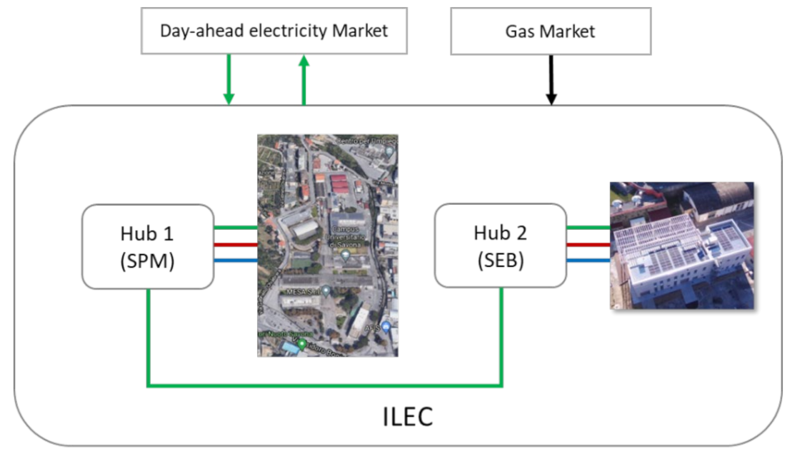
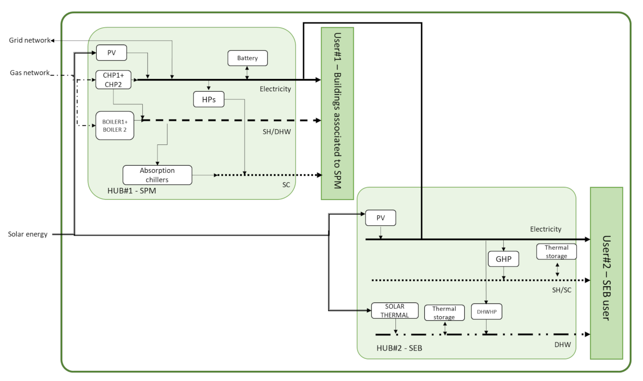
- The campus is treated as an ILEC with two electrically interconnected multi-energy hubs, namely the Smart Polygeneration Microgrid (SPM) and the Smart Energy Building (SEB), involving multiple distributed technologies as PV, solar thermal, CHPs, auxiliary gas-fired boilers, electric and geothermal heat pumps, absorption chillers, electric and thermal storage. Under this prism, the ILEC can also participate in the day-ahead market (DAM) with proper bidding strategies.
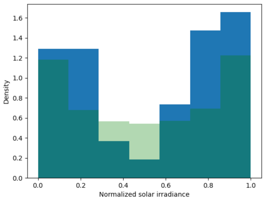
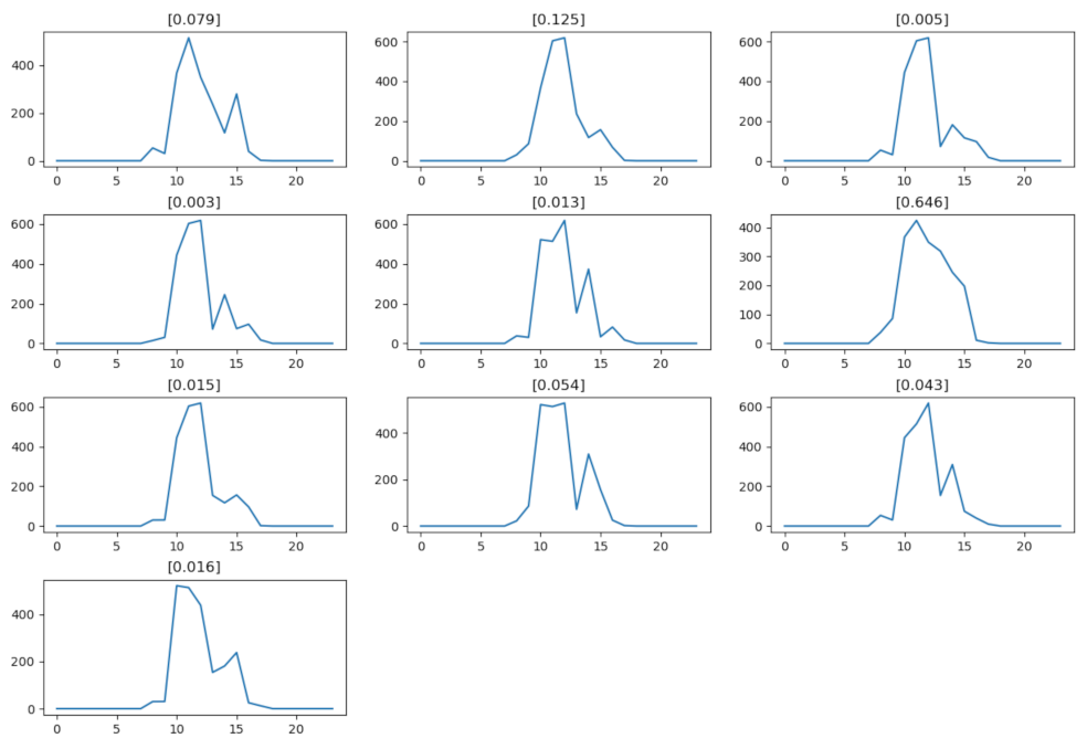
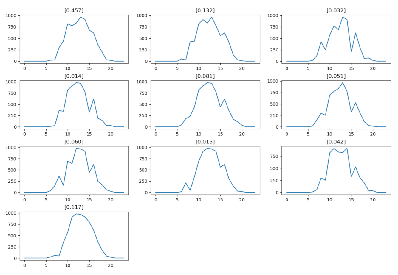
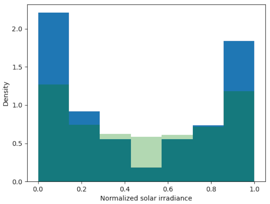
- A stochastic approach is used for the operation optimization model of the campus. To assess the renewables uncertainties, as described in the Appendix A, the roulette wheel method (RWM) is used to generate the initial set of scenarios for daily solar irradiance profiles, and a process of reducing the number of scenarios based on the fast forward selection algorithm is then applied to preserve the most representative scenarios, while reducing the computational load of the subsequent stochastic optimization phase. A stochastic multi-objective optimization model is thus formulated through MILP with the aim to optimize the operation strategies of the various technologies in the ILEC, the electricity exchange between the multi-energy hubs, as well as the bidding strategies of the ILECs in the DAM, considering both energy costs and carbon emissions as objective functions.
1.4. Structure
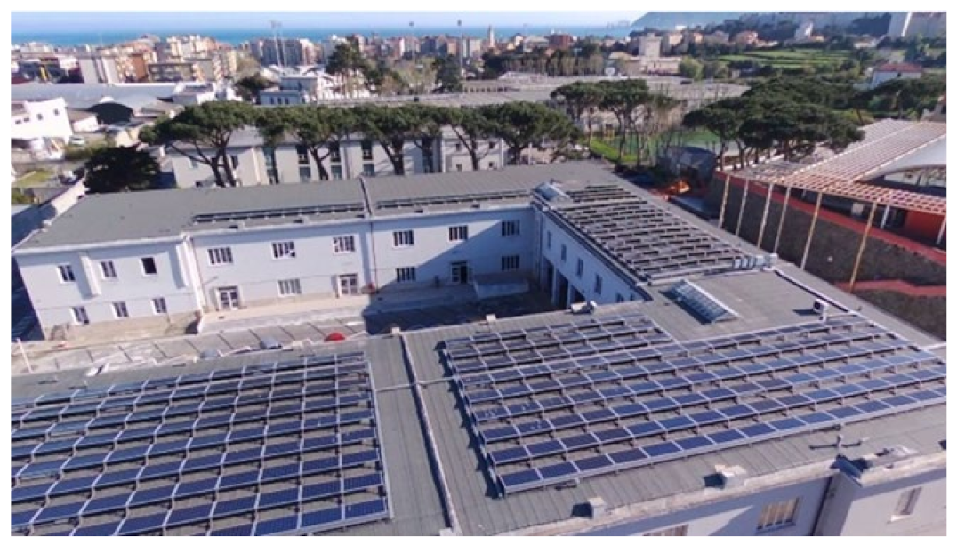
2. The Smart Savona Campus of the University of Genoa
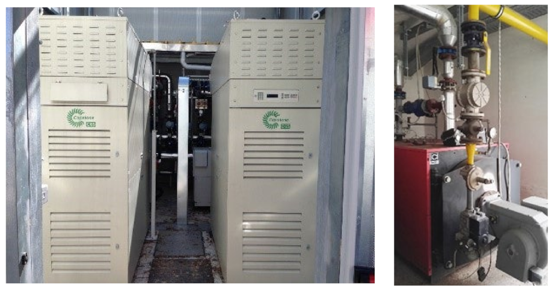
- Two CHP systems with microturbines Capstone C65 as prime movers, fed by natural gas, which are used to provide both electricity and hot water, which is conveyed to the district heating of the campus, thus used for space heating, and space cooling through the absorption chillers.
- Two boilers fed by natural gas with a total thermal rated power of 900 kWth, which are used to feed hot water to the district heating of the campus, and act as secondary priority units with respect to the CHP ones.
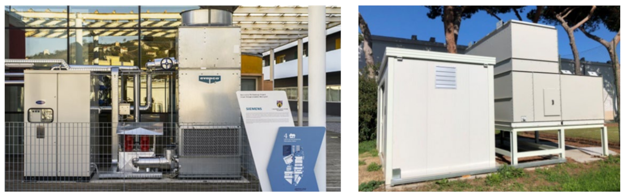
- Two absorption chillers of water/lithium bromide technology, having a cumulative rated cooling power of 220 kWth; they absorb hot water from the microturbines in order to produce cold water (at around 7 °C) which is used for space cooling purposes in several buildings.
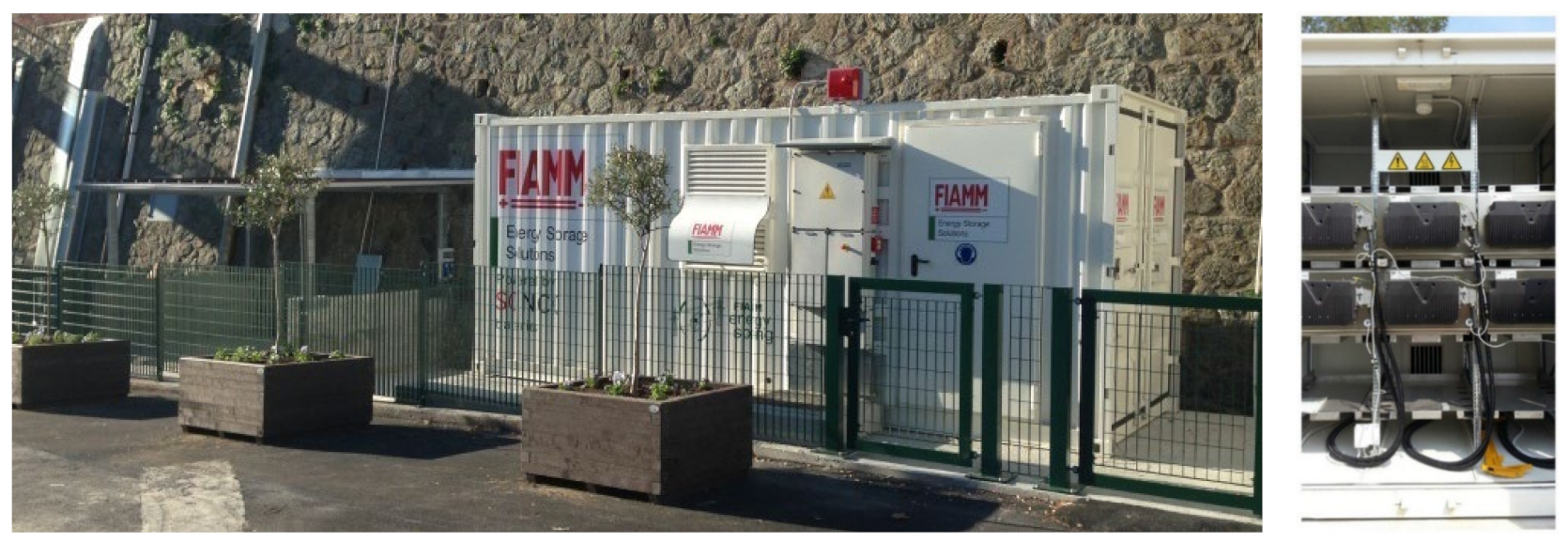
- An electrical storage system, made of six ST523 SoNick batteries with a total nominal capacity of 141 kWh [33], which is mainly used for research purposes and permits the storage of surplus photovoltaic production.
- Several heat pumps (air/water) for a cumulative rated cooling power of 340 kWth, which are used for space cooling of several buildings of the campus such as the new dormitories and two great halls.
- A 21 kWp solar PV plant having 85 polycrystalline silicon panels installed on the flat roof of the building.
- A geothermal heat pump (water/water), having a rated thermal power of 46 kWth, and rated cooling power of 44.3 kWth which is used to satisfy the heating and cooling needs of the building being coupled with a thermal storage of 500 L.
- A domestic hot water heat pump (air/water), having a rated thermal power of 11.5 kWth, which is used, together with solar thermal panels, to satisfy the domestic hot water demand of the building.
- A solar thermal system with two vacuum collectors having a total surface of 3.84 m2. The system is hydraulically connected to the DHW storage tank (having a volume of 500 L) that is equipped with other two heat exchangers, respectively, connected to the geothermal heat pump and to the domestic hot water heat pump.
3. The Mathematical Model and the Optimization Method
3.1. Decision Variables
- On/off status of each energy technology;
- Electric, thermal, and cooling power supplied by each energy technology;
- Electric and thermal power for charging and discharging storage systems;
- Electric power withdrawn from the distribution network;
- Electric power sold on DAM;
- Electric power shared by the SPM to the SEB.
3.2. Modeling of the ILEC
3.2.1. Smart Polygeneration Microgrid
PV Systems
CHP Systems
Auxiliary Gas-Fired Boilers
Electric Heat Pumps
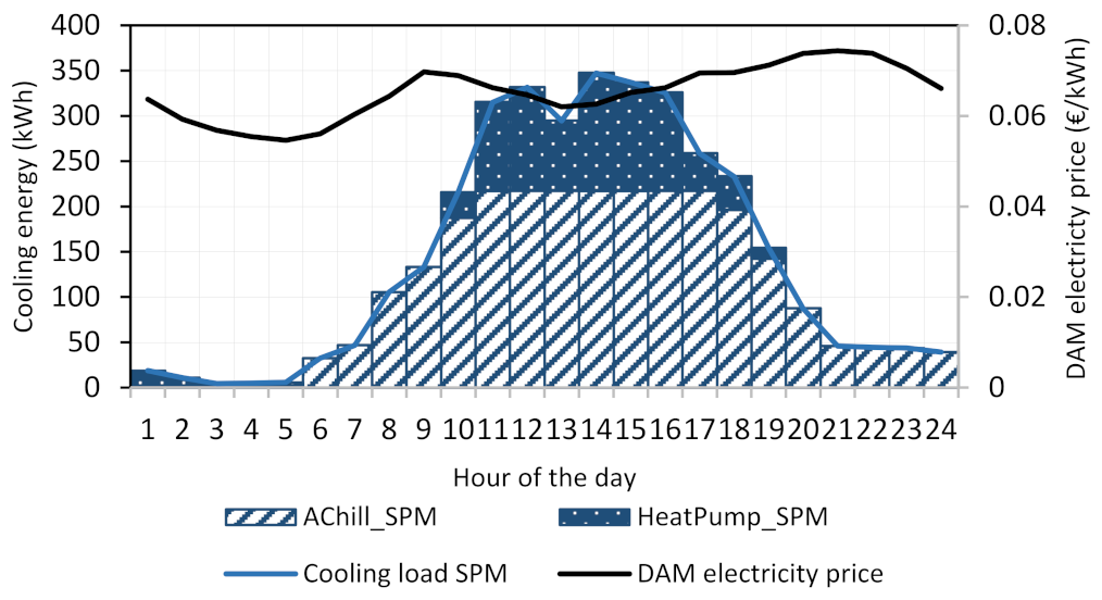
Absorption Chillers
Electric Storage
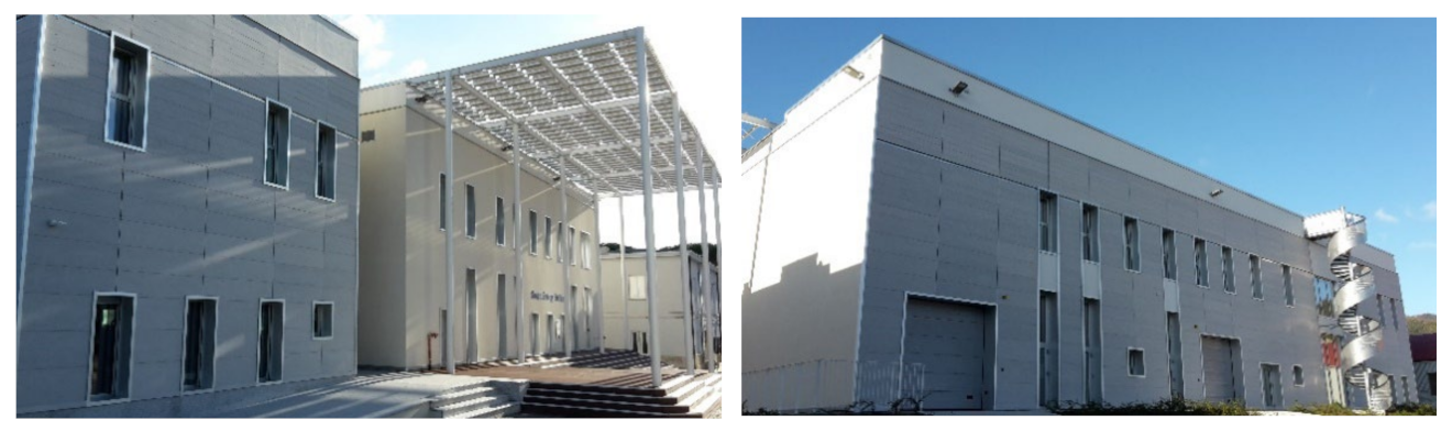
3.2.2. Smart Energy Building
Solar Thermal
Thermal Storage
3.3. Energy Balance Constraints
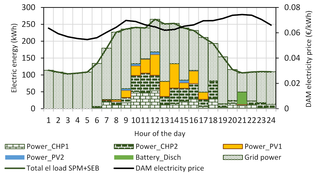
3.3.1. Electric Energy Balance
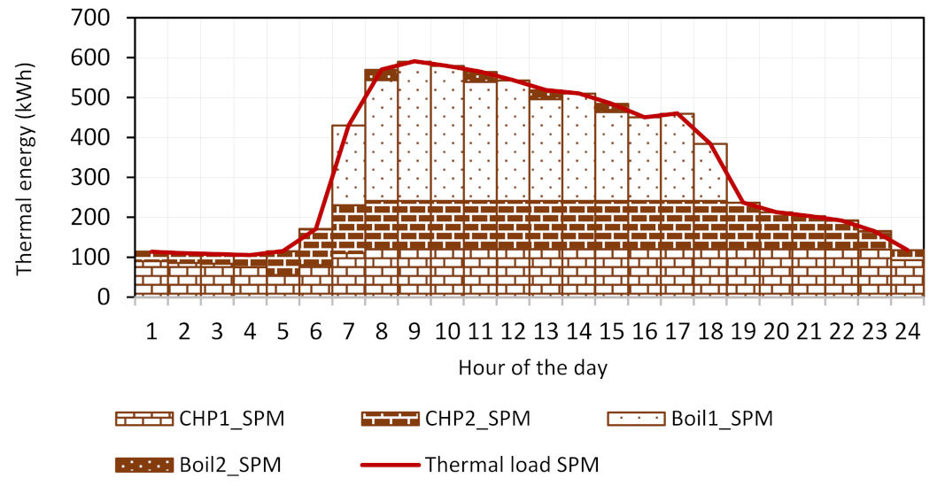
3.3.2. Thermal Energy Balance
SPM
SEB
3.4. Objective Functions
3.5. Multi-Objective Optimization Method
4. Data Analysis for the Smart Savona Campus
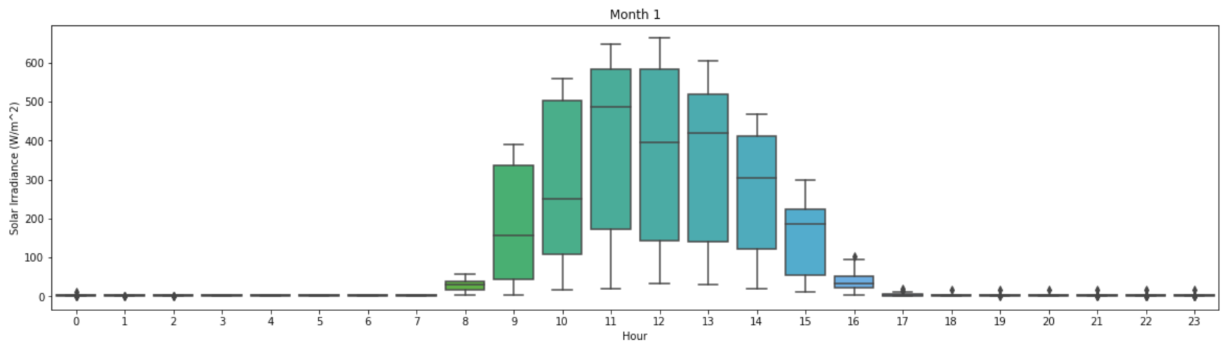
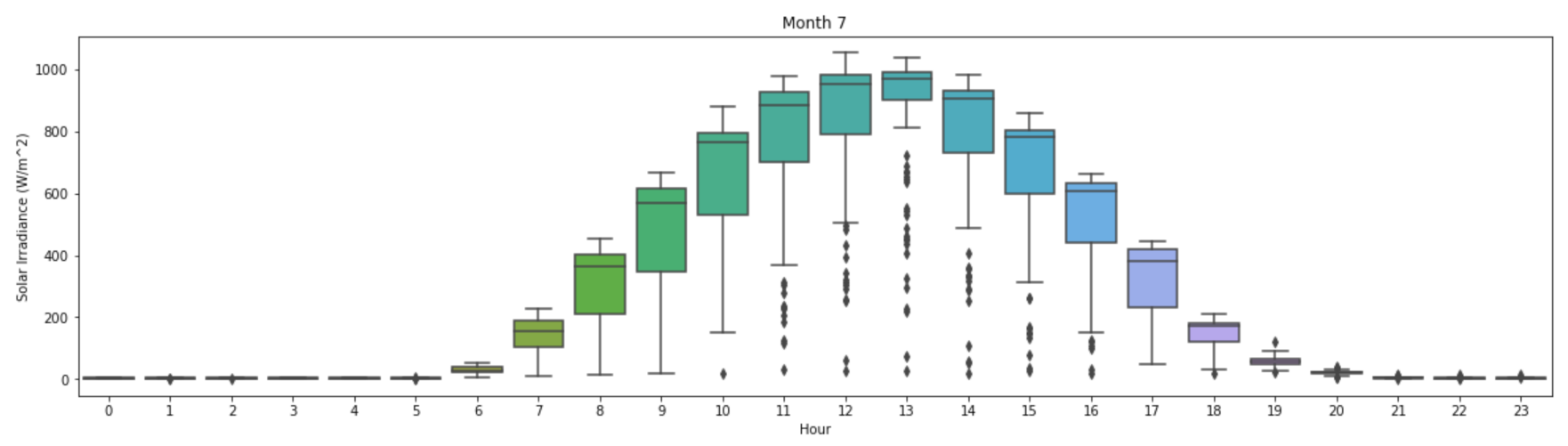
4.1. Definition of Daily Solar Irradiance Profiles
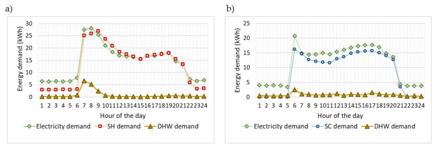
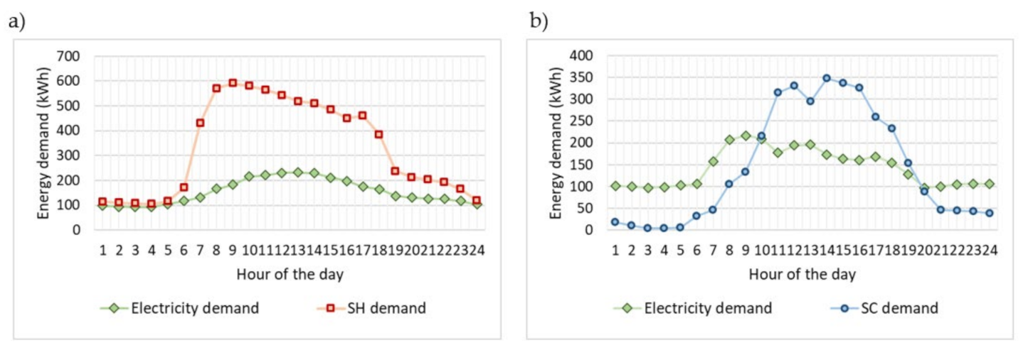
4.2. Energy Demand Profiles
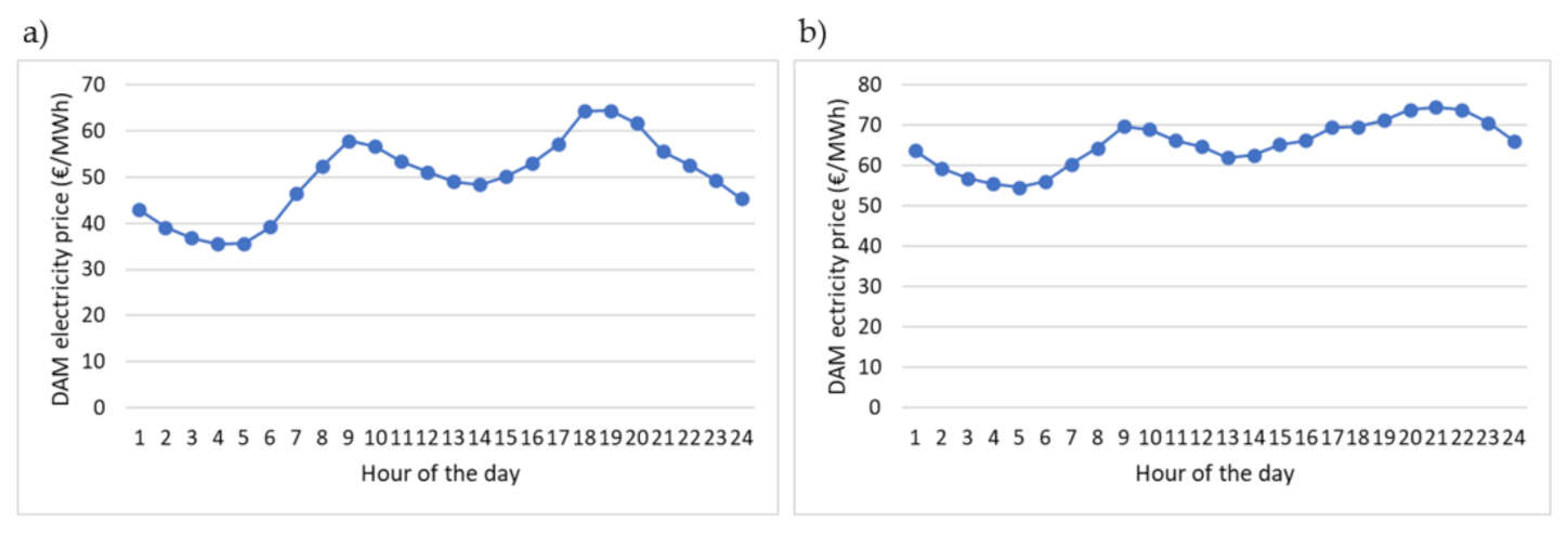
4.3. Other Input Data
5. Analysis of Results
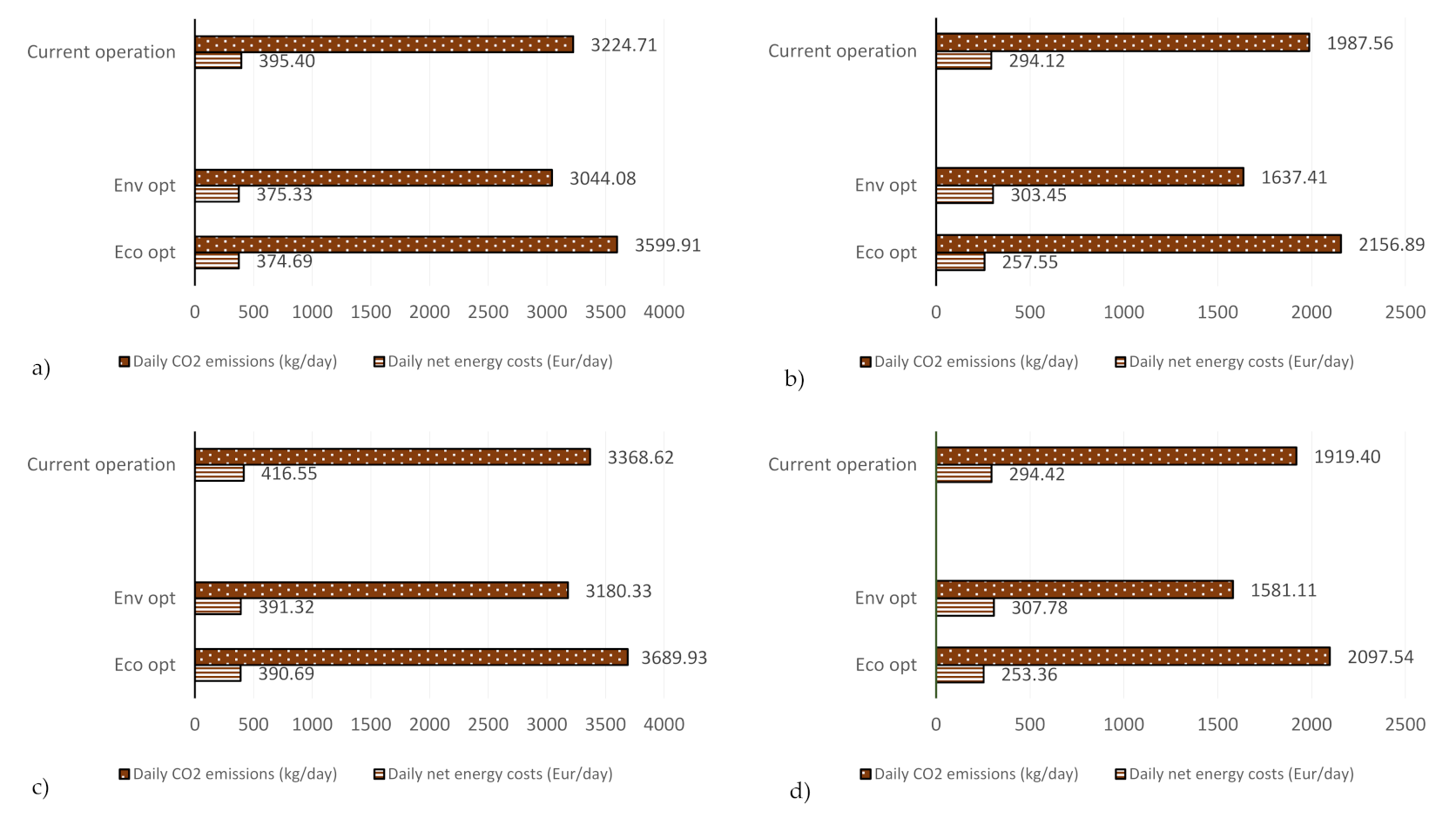
5.1. Economic and Environmental Optimization: Comparison between the Current and the Optimized Case
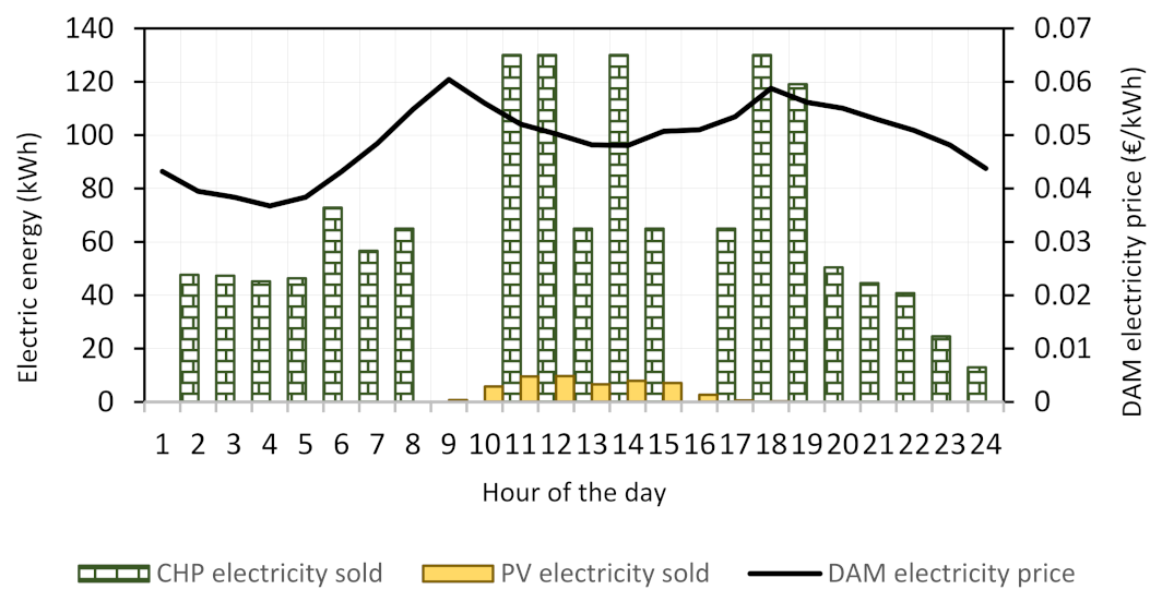
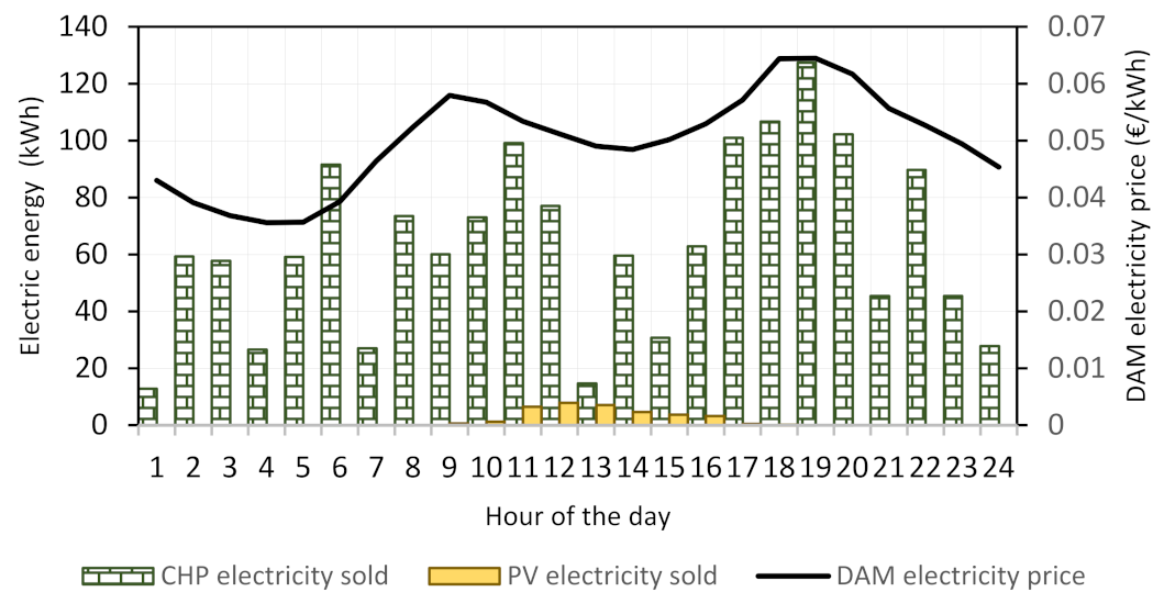
5.2. Bidding Strategies of the ILEC on DAM under the Economic and Environmental Optimization with Stochastic and Deterministic Approach
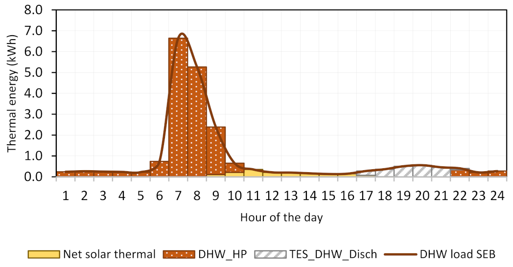
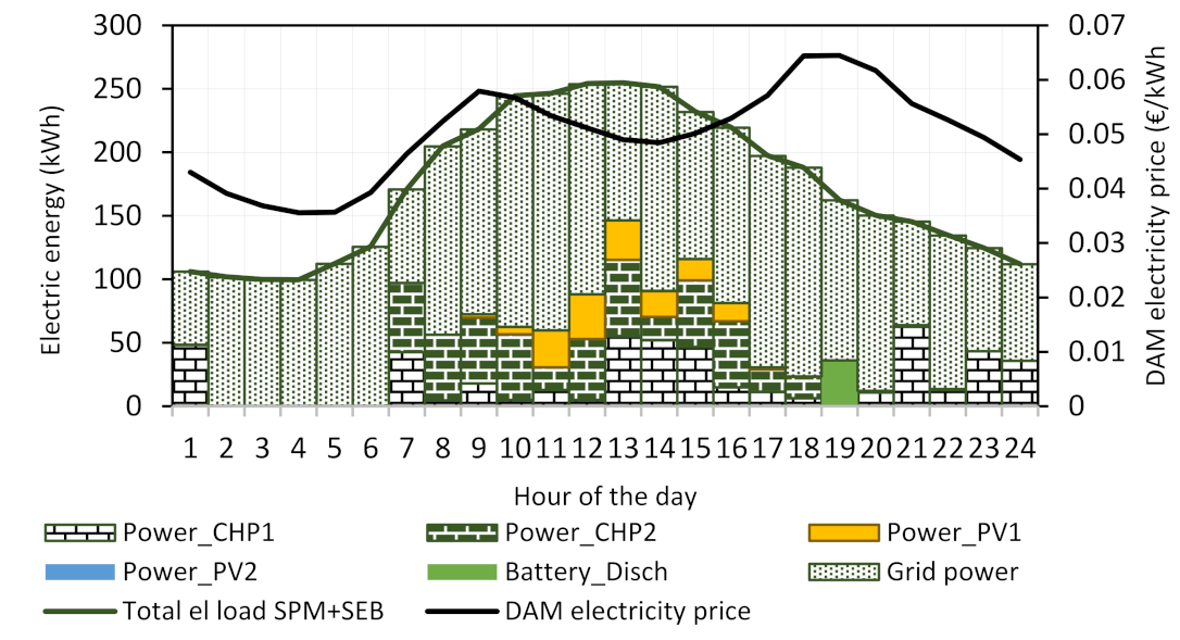
5.3. Energy Balances of the ILEC and Multi-Energy Hubs under the Stochastic Economic and Environmental Optimization
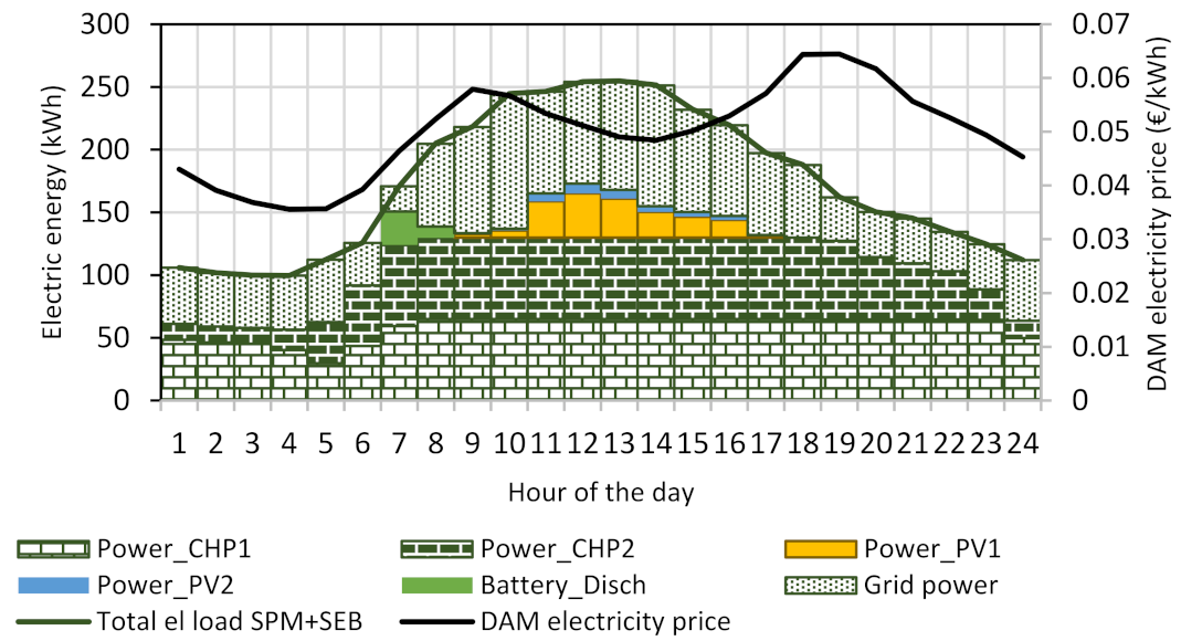
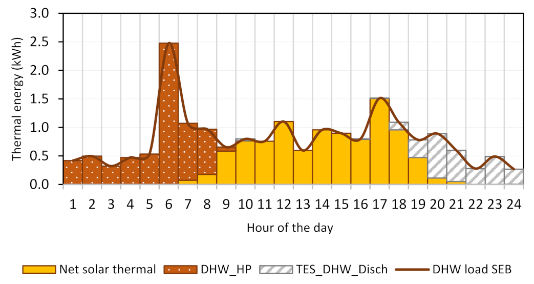
5.3.1. Winter Case
Economic Optimization
Environmental Optimization
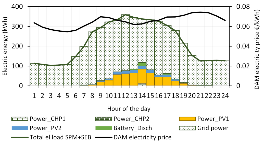
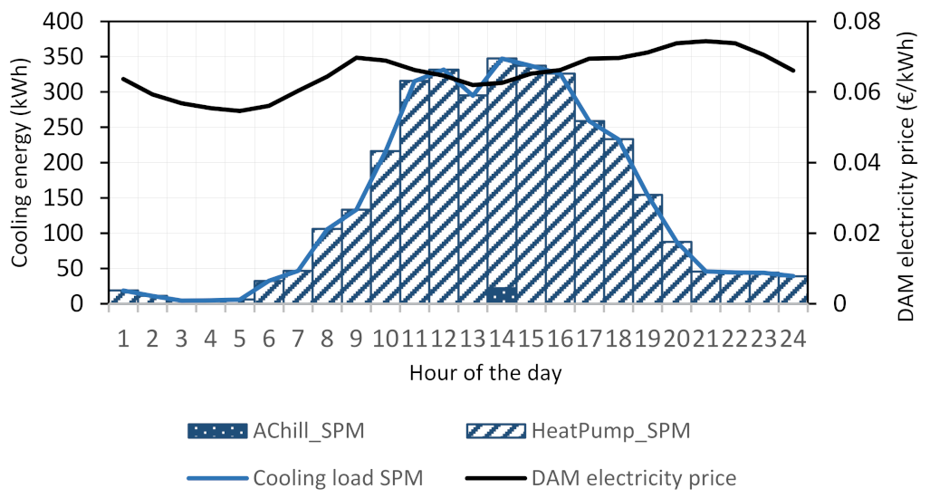
5.3.2. Summer Case
Economic Optimization
Environmental Optimization
6. Conclusions
Author Contributions
Funding
Data Availability Statement
Conflicts of Interest
Nomenclature
| Decision variables | |
| Charging heat rate of TES in scenario s and time t (kW) | |
| Discharging heat rate of TES in scenario s and time t (kW) | |
| Thermal energy of TES in scenario s and time t (kWh) | |
| Charging power of battery in scenario s and time t (kW) | |
| Discharging power of battery in scenario s and time t (kW) | |
| Power bought from DAM in scenario s and time t (kW) | |
| Power required from technology in scenario s and time t (kW) | |
| Power sold on DAM in scenario s and time t (kW) | |
| Binary variable for usage of battery for charging process in scenario s and time t | |
| Binary variable for usage of battery for discharging process in scenario s and time t | |
| Cs,t | Cooling rate provided by technology in scenario s and time t (kW) |
| Fobj,eco | Economic objective function (€) |
| Fobj,env | Environmental objective function (kg CO2) |
| Gs,t | Gas volumetric flow rate in scenario s and time t (Nm3/h) |
| Hs,t | Heat rate provided by technology in scenario s and time t (kW) |
| Ps,t | Power provided by technology in scenario s and time t (kW) |
| SOCBat,s,t | State-of-charge of battery in scenario s and time t |
| xs,t | On/off status of technology in scenario s and time t |
| Parameters | |
| Cooling rate demand of SPM for space cooling at time t (kW) | |
| Heat rate demand of SEB for domestic hot water at time t (kW) | |
| Heat rate demand of SEB for space heating at time t (kW) | |
| Heat rate demand of SPM for space heating and domestic hot water at time t (kW) | |
| Maximum charging power of battery (kW) | |
| Maximum discharging power of battery (kW) | |
| Power demand of user j at time t (kW) | |
| DAM electricity price (€/kWh) | |
| Charging efficiency of battery | |
| Discharging efficiency of battery | |
| Storage loss fraction | |
| APV | Installed PV area (m2) |
| AST | Installed solar thermal area (m2) |
| c | Constant in Equation (24) (kgCO2/€) |
| CapBat | Battery capacity (kWh) |
| COP | Coefficient of performance |
| DRCHP | Maximum ramp-down rate of CHP (kW) |
| Ecin | Carbon intensity of grid power (kgCO2/kWh) |
| Gci | Carbon intensity of gas (kgCO2/Nm3) |
| Is,t | Total solar irradiance in scenario s and time t (kW/m2) |
| LHVgas | Lower heat value of natural gas (kWh/Nm3) |
| np | Number of preserved scenarios |
| nr | Number of regions used to quantize the support of beta distribution |
| ns | Number of generated scenarios |
| Pmax | Capacity of technology (kW) |
| Pmin | Mimimum part load of technology (kW) |
| UR | Maximum ramp-up rate of CHP (kW) |
| Δt | Time interval length (h) |
| ηe | Electric efficiency |
| ηth | Thermal efficiency |
| πs | Probability of occurrence of the scenario s |
| ω | Weight in Equation (24) |
| Πgas | DAM gas price (€/Nm3) |
| Maximum SOC of battery | |
| Minimum SOC of battery | |
| Superscript/Subscripts | |
| AB | Auxiliary boiler |
| AChil | Absorption chiller |
| CHP | Combined heat and power |
| CM | Cooling mode |
| cool | Cooling |
| DAM | Day-ahead market |
| DHW-HP | Domestic hot water heat pump |
| geoHP | Geothermal heat pump |
| heat | Heat |
| HM | Heating mode |
| HP | Heat pump |
| i | Index of technology |
| j | Index of user |
| PV | Photovoltaic |
| s | Index of scenario |
| Self | Self- consumption |
| ST | Solar thermal |
| t | Index of time |
| TES | Thermal energy storage |
| TES-geoHP | Thermal energy storage coupled with geothermal heat pump |
| TES-ST | Thermal energy storage coupled with solar thermal system |
| Acronyms | |
| CHP | Combined heat and power |
| DAM | Day-ahead market |
| ILEC | Integrated local energy community |
| MILP | Mixed-integer linear programming |
| RES | Renewable energy sources |
| RWM | Roulette wheel method |
| SEB | Smart energy building |
| SPM | Smart polygeneration microgrid |
Appendix A. Modeling of RES Uncertainties through the Scenario Generation Method
References
- A European Green Deal Striving to be the First Climate-Neutral Continent. Available online: https://ec.europa.eu/info/strategy/priorities-2019-2024/european-green-deal_en (accessed on 1 August 2022).
- Di Somma, M.; Graditi, G. Challenges and Opportunities of the Energy Transition and the Added Value of Energy Systems Integration. Technol. Integr. Energy Syst. Netw. 2022, 1–14. [Google Scholar] [CrossRef]
- ETIP SNET. Sector Coupling: Concepts, State-of-the-Art and Perspectives. White Paper. January 2020. Available online: https://orbi.uliege.be/bitstream/2268/244983/2/ETIP-SNEP-Sector-Coupling-Concepts-state-of-the-art-and-perspectives-WG1.pdf (accessed on 1 August 2022).
- ETIP SNET VISION 2050. Integrating Smart Networks for the Energy Transition: Serving Society and Protecting the Environment, Report. 2017. Available online: https://smart-networks-energy-transition.ec.europa.eu/publications/etip-publications (accessed on 1 August 2022).
- Yan, B.; Di Somma, M.; Luh, P.B.; Graditi, G. Operation optimization of multiple distributed energy systems in an energy community. In Proceedings of the 2018 IEEE International Conference on Environment and Electrical Engineering and 2018 IEEE Industrial and Commercial Power Systems Europe (EEEIC/I&CPS Europe), Palermo, Italy, 12–15 June 2018. [Google Scholar]
- Foiadelli, F.; Nocerino, S.; Di Somma, M.; Graditi, G. Optimal design of DER for economic/environmental sustainability of local energy communities. In Proceedings of the 2018 IEEE International Conference on Environment and Electrical Engineering and 2018 IEEE Industrial and Commercial Power Systems Europe (EEEIC/I&CPS Europe), Palermo, Italy, 12–15 June 2018; pp. 1–7. [Google Scholar]
- Caliano, M.; Bianco, N.; Graditi, G.; Mongibello, L. Economic optimization of a residential micro-CHP system considering different operation strategies. Appl. Therm. Eng. 2016, 101, 592–600. [Google Scholar] [CrossRef]
- Hawkes, A.D.; Leach, M.A. Cost-effective operating strategy for residential micro-combined heat and power. Energy 2007, 32, 711–723. [Google Scholar] [CrossRef]
- Shaneb, O.A.; Taylor, P.C.; Coates, G. Optimal online operation of residential μCHP systems using linear programming. Energy Build. 2012, 44, 17–25. [Google Scholar] [CrossRef]
- Kong, X.Q.; Wang, R.Z.; Li, Y.; Huang, X.H. Optimal operation of a micro-combined cooling, heating and power system driven by a gas engine. Energy Convers. Manag. 2009, 50, 530–538. [Google Scholar] [CrossRef]
- Gao, Y.; Deng, Y.; Yao, W.; Hang, Y. Optimization of combined cooling, heating, and power systems for rural scenario based on a two-layer optimization model. J. Build. Eng. 2022, 60, 105217. [Google Scholar] [CrossRef]
- Ren, H.; Zhou, W.; Nakagami, K.I.; Gao, W.; Wu, Q. Multi-objective optimization for the operation of distributed energy systems considering economic and environmental aspects. Appl. Energy 2010, 87, 3642–3651. [Google Scholar] [CrossRef]
- Shabanpour-Haghighi, A.; Seifi, A.R. Multi-objective operation management of a multi-carrier energy system. Energy 2015, 88, 430–442. [Google Scholar] [CrossRef]
- Mohammadi, S.; Soleymani, S.; Mozafari, B. Scenario-based stochastic operation management of microgrid including wind, photovoltaic, micro-turbine, fuel cell and energy storage devices. Int. J. Electr. Power Energy Syst. 2014, 54, 525–535. [Google Scholar] [CrossRef]
- Di Somma, M.; Graditi, G.; Heydarian-Forushani, E.; Shafie-khah, M.; Siano, P. Stochastic optimal scheduling of distributed energy resources with renewables considering economic and environmental aspects. Renew. Energy 2018, 116, 272–287. [Google Scholar] [CrossRef]
- Liu, Y.; Gooi, H.B.; Li, Y.; Xin, H.; Ye, J. A Secure Distributed Transactive Energy Management Scheme for Multiple Interconnected Microgrids Considering Misbehaviors. IEEE Trans. Smart Grid 2019, 10, 5975–5986. [Google Scholar] [CrossRef]
- Wang, Z.; Chen, B.; Wang, J.; Begovic, M.M.; Chen, C. Coordinated energy management of networked microgrids in distribution systems. IEEE Trans. Smart Grid 2014, 6, 45–53. [Google Scholar] [CrossRef]
- Wu, J.; Guan, X. Coordinated multi-microgrids optimal control algorithm for smart distribution management system. IEEE Trans. Smart Grid 2013, 4, 2174–2181. [Google Scholar] [CrossRef]
- Lan, Y.; Guan, X.; Wu, J. Online decentralized and cooperative dispatch for multi-microgrids. IEEE Trans. Autom. Sci. 2019, 17, 450–462. [Google Scholar] [CrossRef]
- Parisio, A.; Wiezorek, C.; Kyntäjä, T.; Elo, J.; Strunz, K.; Johansson, K.H. Cooperative MPC-based energy management for networked microgrids. IEEE Trans. Smart Grid 2017, 8, 3066–3074. [Google Scholar] [CrossRef]
- Yan, B.; Di Somma, M.; Graditi, G.; Luh, P.B. Markovian-based stochastic operation optimization of multiple distributed energy systems with renewables in a local energy community. Electr. Power Syst. Res. 2020, 186, 106364. [Google Scholar] [CrossRef]
- Delfino, F.; Ferro, G.; Robba, M.; Rossi, M. An Energy Management Platform for the Optimal Control of Active and Reactive Power in Sustainable Microgrids. IEEE Trans. Ind. Appl. 2019, 55, 7146–7156. [Google Scholar] [CrossRef]
- Delfino, F.; Ferro, G.; Parodi, L.; Robba, M.; Rossi, M.; Caliano, M.; Di Somma, M.; Graditi, G. A multi-objective Energy Management System for microgrids: Minimization of costs, exergy in input, and emissions. In Proceedings of the International Conference on Smart Energy Systems and Technologies (SEST), Eindhoven, The Netherlands, 5–7 September 2021; pp. 1–6. [Google Scholar]
- Bracco, S.; Delfino, F.; Pampararo, F.; Robba, M.; Rossi, M. A mathematical model for the optimal operation of the University of Genoa Smart Polygeneration Microgrid: Evaluation of technical, economic and environmental performance indicators. Energy 2014, 64, 912–922. [Google Scholar] [CrossRef]
- Bracco, S.; Brignone, M.; Delfino, F.; Procopio, R. An energy management system for the savona campus smart polygeneration microgrid. IEEE Syst. J. 2015, 11, 1799–1809. [Google Scholar] [CrossRef]
- Bracco, S.; Delfino, F.; Rossi, M.; Robba, M. A multi-objective optimization tool for the daily management of sustainable smart microgrids: Case Study: The savona campus SPM and SEB facilities. In Proceedings of the 2016 International Symposium on Power Electronics, Electrical Drives, Automation and Motion (SPEEDAM), Capri Island, Italy, 22–24 June 2016; pp. 683–688. [Google Scholar]
- Bracco, S.; Brignone, M.; Delfino, F.; Pampararo, F.; Rossi, M.; Ferro, G.; Robba, M. An Optimization Model for Polygeneration Microgrids with Renewables, Electrical and Thermal Storage: Application to the Savona Campus. In Proceedings of the EEEIC/I&CPS Europe, Palermo, Italy, 6 December 2018; pp. 1–6. [Google Scholar]
- Bracco, S.; Delfino, F.; Laiolo, P.; Morini, A. Planning & Open-Air Demonstrating Smart City Sustainable Districts. Sustainability 2018, 10, 4636. [Google Scholar]
- University of Genoa Savona Campus Webpage. Available online: https://campus-savona.unige.it/en/ (accessed on 15 November 2021).
- University of Genoa Energia 2020 Project. Available online: http://www.energia2020.unige.it/en/home/ (accessed on 15 November 2021).
- Bracco, S.; Delfino, F.; Piazza, G.; de Simón-Martín, M. V2G Technology to Mitigate PV Uncertainties. In Proceedings of the Fifteenth International Conference on Ecological Vehicles and Renewable Energies (EVER), Monte Carlo, Monaco, 28 May 2020; pp. 1–6. [Google Scholar]
- Bracco, S.; Delfino, F.; Foiadelli, F.; Longo, M. Smart Microgrid Monitoring: Evaluation of Key Performance Indicators for a PV Plant Connected to a LV Microgrid. In Proceedings of the IEEE PES Innovative Smart Grid Technologies Conference Europe (ISGT-Europe), Torino, Italy, 23–26 October 2017; pp. 1–6. [Google Scholar]
- Bracco, S.; Delfino, F.; Trucco, A.; Zin, S. Electrical storage systems based on Sodium/Nickel chloride batteries: A mathematical model for the cell electrical parameter evaluation validated on a real smart microgrid application. J. Power Sources 2018, 399, 372–382. [Google Scholar] [CrossRef]
- De Simón-Martín, M.; Bracco, S.; Piazza, G.; Pagnini, L.C.; González-Martínez, A.; Delfino, F. Application to Real Case Studies. In Levelized Cost of Energy in Sustainable Energy Communities; SpringerBriefs in Applied Sciences and Technology; Springer: Cham, Switzerland, 2022. [Google Scholar]
- Delfino, F.; Procopio, R.; Rossi, M.; Brignone, M.; Robba, M.; Bracco, S. Microgrid Design and Operation. Toward Smart Energy in Cities; Artech House: Norwood, MA, USA, 2018. [Google Scholar]
- Deb, K. Multi-Objective Optimization Using Evolutionary Algorithms; John Wiley and Sons: Hoboken, NJ, USA, 2001; ISBN 047187339X. [Google Scholar]
- Alarcon-Rodriguez, A.; Ault, G.; Galloway, S. Multi-objective planning of distributed energy resources: A review of the state-of-the-art. Renew. Renew. Sustain. Energy Rev. 2010, 14, 1353–1366. [Google Scholar] [CrossRef]
- Buonanno, A.; Caliano, M.; Di Somma, M.; Graditi, G.; Valenti, M. Comprehensive Method for Modeling Uncertainties of Solar Irradiance for PV Power Generation in Smart Grids. In Proceedings of the International Conference on Smart Energy Systems and Technologies (SEST), Vaasa, Finland, 6–8 September 2021. [Google Scholar]
- Murphy, K.P. Machine Learning: A Probabilistic Perspective; MIT Press: Cambridge, MA, USA, 2012; pp. 62–63. [Google Scholar]
- Michalewicz, Z. Genetic Algorithms + Data Structures = Evolution Programs; Springer: Berlin/Heidelberg, Germany, 1996. [Google Scholar]
- Growe-Kuska, N.; Heitsch, H.; Roemisch, W. Scenario Reduction and Scenario Tree Construction for Power Management Problems. In Proceedings of the 2003 IEEE Bologna Power Tech Conference Proceedings, Bologna, Italy, 23–26 June 2003. [Google Scholar]
- Data from Italian Energy Market. Available online: http://www.mercatoelettrico.org/it/ (accessed on 3 September 2021).


| Energy Hub | Technology | Size | Efficiency | |
|---|---|---|---|---|
| Electric | Thermal | |||
| Hub 1-SPM | PV systems | 95 kWp (total) | 0.13 | |
| CHP MGT (×2) | 65 kWel–112 kWth | 0.28 | 0.50 | |
| Gas-fired boilers (×2) | 900 kW (total) | 0.80 | ||
| Electric heat pumps | 135 kWel–340 kWth (total) | COPSC = 2.3 | ||
| Absorption chillers | 220 kWth (total) | COP = 0.90 | ||
| Electricity storage | 141 kWh | = 0.86 | ||
| Hub 2-SEB | PV | 21 kWp | 0.14 | |
| Geothermal HP | 46 kWth | COPGHP = 4.4 | ||
| Thermal storage | 500 L | 0.90 | ||
| DHW HP | 11.5 kWth | COPSH = 2.8 | ||
| Solar thermal | 3.84 m2 | 0.72 | ||
Publisher’s Note: MDPI stays neutral with regard to jurisdictional claims in published maps and institutional affiliations. |
© 2022 by the authors. Licensee MDPI, Basel, Switzerland. This article is an open access article distributed under the terms and conditions of the Creative Commons Attribution (CC BY) license (https://creativecommons.org/licenses/by/4.0/).
Share and Cite
Di Somma, M.; Buonanno, A.; Caliano, M.; Graditi, G.; Piazza, G.; Bracco, S.; Delfino, F. Stochastic Operation Optimization of the Smart Savona Campus as an Integrated Local Energy Community Considering Energy Costs and Carbon Emissions. Energies 2022, 15, 8418. https://doi.org/10.3390/en15228418
Di Somma M, Buonanno A, Caliano M, Graditi G, Piazza G, Bracco S, Delfino F. Stochastic Operation Optimization of the Smart Savona Campus as an Integrated Local Energy Community Considering Energy Costs and Carbon Emissions. Energies. 2022; 15(22):8418. https://doi.org/10.3390/en15228418
Chicago/Turabian StyleDi Somma, Marialaura, Amedeo Buonanno, Martina Caliano, Giorgio Graditi, Giorgio Piazza, Stefano Bracco, and Federico Delfino. 2022. "Stochastic Operation Optimization of the Smart Savona Campus as an Integrated Local Energy Community Considering Energy Costs and Carbon Emissions" Energies 15, no. 22: 8418. https://doi.org/10.3390/en15228418
APA StyleDi Somma, M., Buonanno, A., Caliano, M., Graditi, G., Piazza, G., Bracco, S., & Delfino, F. (2022). Stochastic Operation Optimization of the Smart Savona Campus as an Integrated Local Energy Community Considering Energy Costs and Carbon Emissions. Energies, 15(22), 8418. https://doi.org/10.3390/en15228418