
A Numerical Study on an Oscillating Water Column Wave Energy Converter with Hyper-Elastic Material


Abstract
1. Introduction
2. Numerical Method
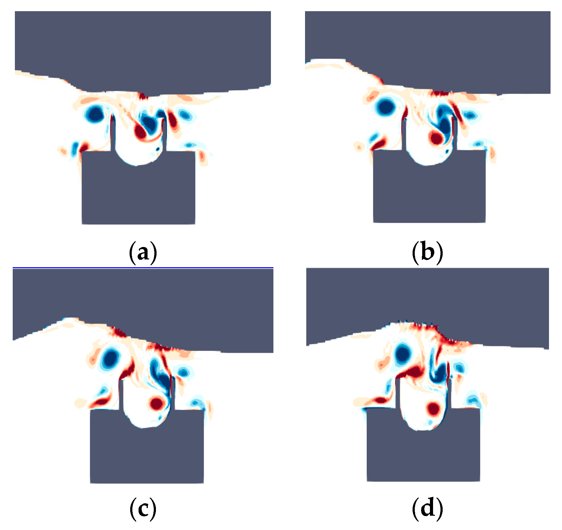
2.1. Fluid Solver
2.2. Structural Solver
2.3. Coupling Scheme
3. Results and Discussion
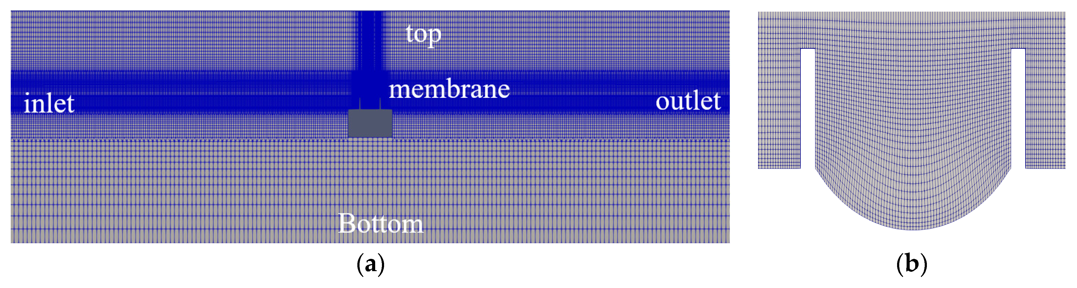
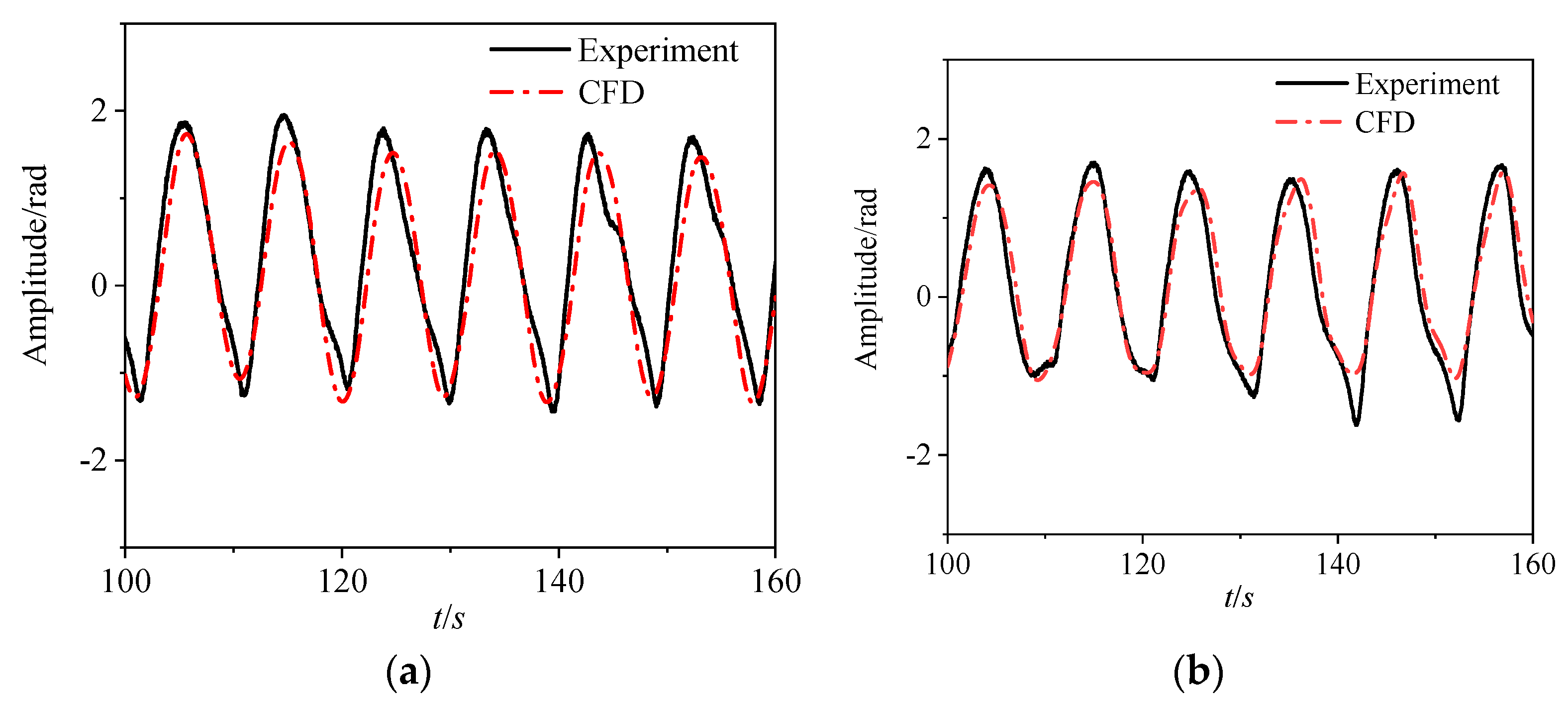
3.1. Grid and Time Step Sensitivity Study and Numerical Method Validation
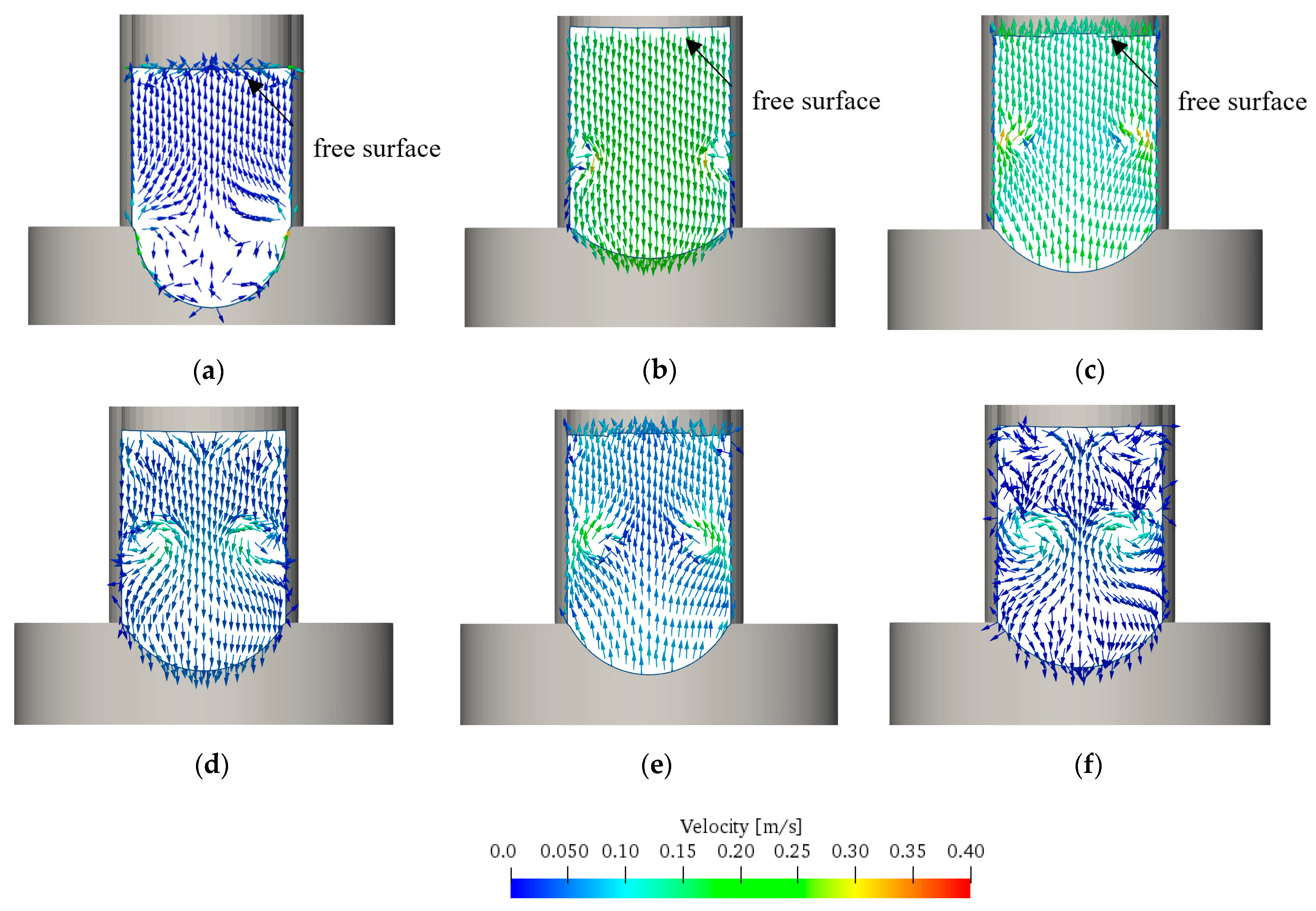
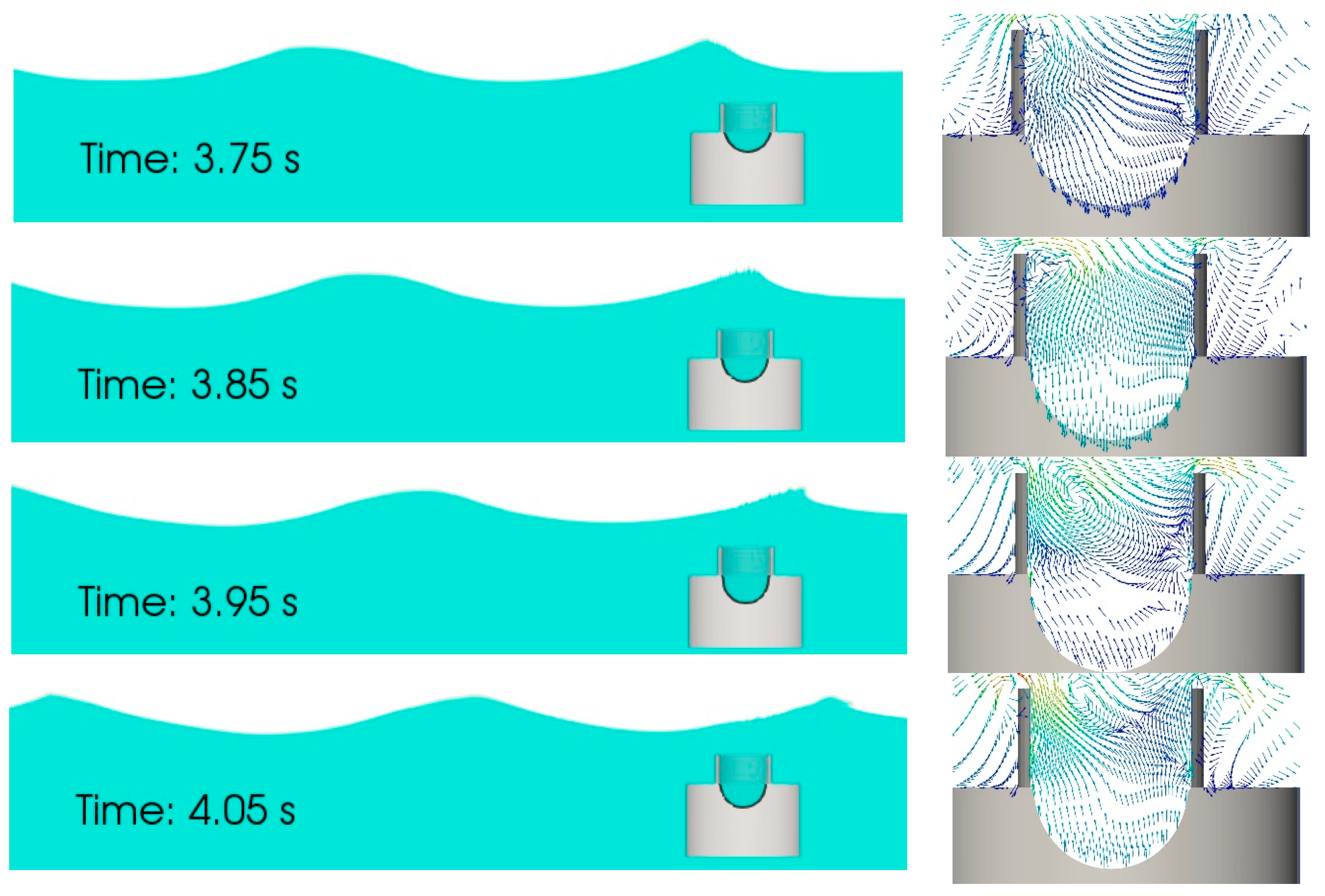
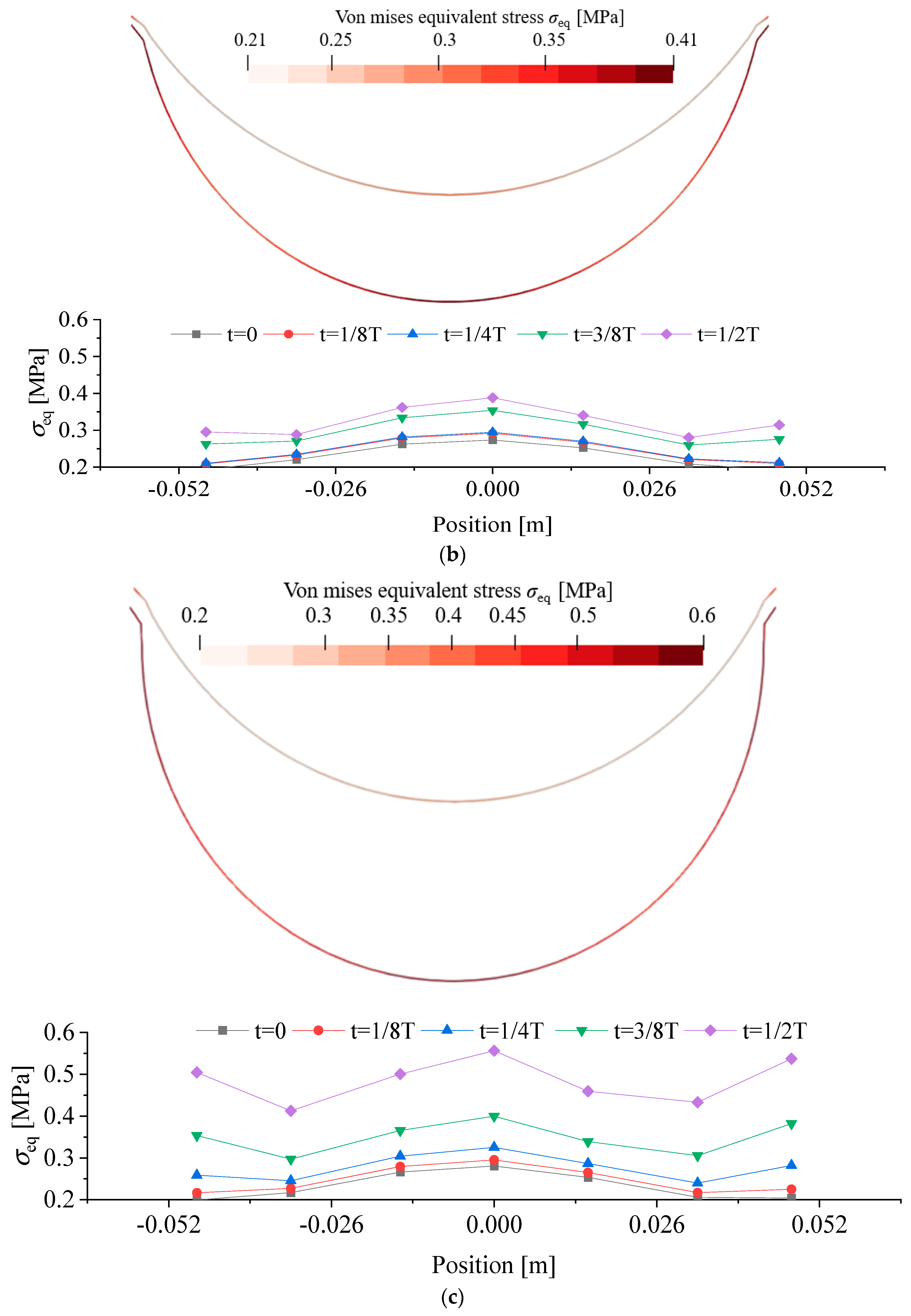
3.2. Role of Hydrostatic and Hydrodynamic Pressure on the Membrane’s Deformation
3.3. Response of Membrane Deformation under Hydrostatic Pressure
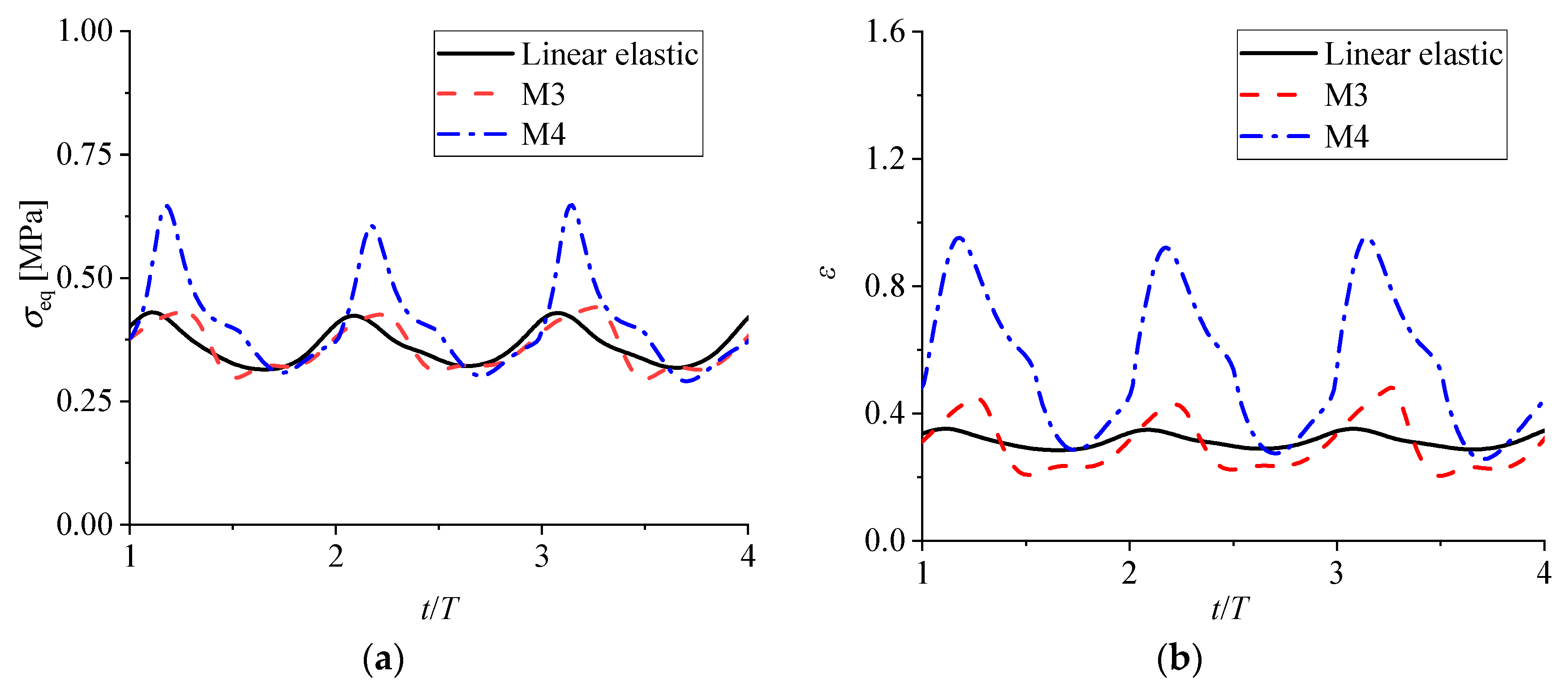
3.4. Response of Membrane Deformation under Hydrodynamic Pressure: Material Impact
3.5. Response of Membrane Deformation under Hydrodynamic Pressure: Wave Period Impact
4. Conclusions
Author Contributions
Funding
Acknowledgments
Conflicts of Interest
References
- Henderson, R. Design, simulation, and testing of a novel hydraulic power take-off system for the Pelamis wave energy converter. Renew. Energy 2006, 31, 271–283. [Google Scholar]
- Cameron, L.; Doherty, R.; Henry, A.; Doherty, K.; Van’t Hoff, J.; Kaye, D.; Naylor, D.; Bourdier, S.; Whittaker, T. Design of the next generation of the Oyster wave energy converter. In Proceedings of the ICOE 2010 Bilbao—International Conference on Ocean Energy, Bilbao, Spain, 6–8 October 2010; p. 1e12. [Google Scholar]
- Li, X.; Xiao, Q.; Zhou, Y.; Ning, D.; Incecik, A.; Nicoll, R.; McDonald, A.; Campbell, D. Coupled CFD-MBD numerical modeling of a mechanically coupled WEC array. Ocean. Eng. 2022, 256, 111541. [Google Scholar] [CrossRef]
- Falcão, A.F.O.; Justino, P. OWC wave energy devices with air flow control. Ocean. Eng. 1999, 26, 1275–1295. [Google Scholar] [CrossRef]
- Ning, D.-Z.; Wang, R.-Q.; Zou, Q.-P.; Teng, B. An experimental investigation of hydrodynamics of a fixed OWC Wave Energy Converter. Appl. Energy 2016, 168, 636–648. [Google Scholar] [CrossRef]
- Wang, R.; Ning, D. Dynamic analysis of wave action on an OWC wave energy converter under the influence of viscosity. Renew. Energy 2020, 150, 578–588. [Google Scholar]
- Zhao, W.; Wolgamot, H.; Taylor, P.; Taylor, R.E. Gap resonance and higher harmonics driven by focused transient wave groups. J. Fluid Mech. 2017, 812, 905–939. [Google Scholar] [CrossRef]
- Yu, X.; Chwang, A.T. Wave-induced oscillation in harbor with porous breakwaters. J. Waterw. Port Coast. Ocean. Eng. 1994, 120, 125–144. [Google Scholar] [CrossRef]
- Rosati Papini, G.P.; Moretti, G.; Vertechy, R.; Fontana, M. Control of an oscillating water column wave energy converter based on dielectric elastomer generator. Nonlinear Dyn. 2018, 92, 181–202. [Google Scholar]
- Collins, I.; Hossain, M.; Dettmer, W.; Masters, I. Flexible membrane structures for wave energy harvesting: A review of the developments, materials and computational modelling approaches. Renew. Sustain. Energy Rev. 2021, 151, 111478. [Google Scholar] [CrossRef]
- Moretti, G.; Santos Herran, M.; Forehand, D.; Alves, M.; Jeffrey, H.; Vertechy, R.; Fontana, M. Advances in the development of dielectric elastomer generators for wave energy conversion. Renew. Sustain. Energy Rev. 2020, 117, 109430. [Google Scholar] [CrossRef]
- Moretti, G.; Papini, G.P.R.; Righi, M.; Forehand, D.; Ingram, D.; Vertechy, R.; Fontana, M. Resonant wave energy harvester based on dielectric elastomer generator. Smart Mater. Struct. 2018, 27, 035015. [Google Scholar] [CrossRef]
- Moretti, G.; Fontana, M.; Vertechy, R. Model-based design and optimization of a dielectric elastomer power take-off for oscillating wave surge energy converters. Meccanica 2015, 50, 2797–2813. [Google Scholar] [CrossRef]
- Michailides, C.; Angelides, D.C. Optimization of a flexible floating structure for wave energy production and protection effectiveness. Eng. Struct. 2015, 85, 249–263. [Google Scholar] [CrossRef]
- Babarit, A.; Singh, J.; Mélis, C.; Wattez, A.; Jean, P. A linear numerical model for analysing the hydroelastic response of a flexible electroactive wave energy converter. J. Fluids Struct. 2017, 74, 356–384. [Google Scholar] [CrossRef]
- Farley, F.; Rainey, R.; Chaplin, J. Rubber tubes in the sea. Philos. Trans. R. Soc. A Math. Phys. Eng. Sci. 2012, 370, 381–402. [Google Scholar] [CrossRef]
- Chaplin, J.; Heller, V.; Farley, F.; Hearn, G.; Rainey, R. Laboratory testing the Anaconda. Philos. Trans. R. Soc. A Math. Phys. Eng. Sci. 2012, 370, 403–424. [Google Scholar] [CrossRef]
- Kurniawan, A.; Chaplin, J.; Greaves, D.; Hann, M. Wave energy absorption by a floating air bag. J. Fluid Mech. 2017, 812, 294–320. [Google Scholar]
- Renzi, E. Hydroelectromechanical modelling of a piezoelectric wave energy converter. Proc. R. Soc. A Math. Phys. Eng. Sci. 2016, 472, 20160715. [Google Scholar] [CrossRef]
- Zheng, S.; Greaves, D.; Meylan, M.H.; Iglesias, G. Wave Power Extraction by a Submerged Piezoelectric Plate; Developments in Renewable Energies Offshore; CRC Press: Boca Raton, FL, USA, 2020. [Google Scholar]
- King, A.; Algie, C.; Ryan, S.; Ong, R. Modelling of fluid structure interactions in submerged flexible membranes for the bombora wave energy converter. In Proceedings of the 20th Australasian Fluid Mechanics Conference, Perth, Australia, 5–8 December 2016. [Google Scholar]
- Li, X.; Xiao, Q.; Luo, Y.; Moretti, G.; Fontana, M.; Righi, M. Dynamic response of a novel flexible wave energy converter under regular waves. In Proceedings of the 14th European Wave and Tidal Energy Conference, Plymouth, UK, 5–9 September 2021; pp. 1–7. [Google Scholar]
- Causin, P.; Gerbeau, J.F.; Nobile, F. Added-mass effect in the design of partitioned algorithms for fluid–structure problems. Comput. Methods Appl. Mech. Eng. 2005, 194, 4506–4527. [Google Scholar] [CrossRef]
- Bungartz, H.-J.; Lindner, F.; Gatzhammer, B.; Mehl, M.; Scheufele, K.; Shukaev, A.; Uekermann, B. preCICE–a fully parallel library for multi-physics surface coupling. Comput. Fluids 2016, 141, 250–258. [Google Scholar]
- Jasak, H.; Jemcov, A.; Tukovic, Z. OpenFOAM: A C++ library for complex physics simulations. In Proceedings of the International Workshop on Coupled Methods in Numerical Dynamics, IUC, Dubrovnik, Croatia, 19–21 September 2007; pp. 1–20. [Google Scholar]
- Hirt, C.W.; Nichols, B.D. Volume of fluid (VOF) method for the dynamics of free boundaries. J. Comput. Phys. 1981, 39, 201–225. [Google Scholar] [CrossRef]
- Dingemans, M.W. Water Wave Propagation over Uneven Bottoms: Linear Wave Propagation; World Scientific: Singapore, 1997; Volume 13. [Google Scholar]
- Dhondt, G. The Finite Element Method for Three-Dimensional Thermomechanical Applications; John Wiley & Sons: Hoboken, NJ, USA, 2004. [Google Scholar]
- Luo, Y.; Xiao, Q.; Zhu, Q.; Pan, G. Jet propulsion of a squid-inspired swimmer in the presence of background flow. Phys. Fluids 2021, 33, 031909. [Google Scholar] [CrossRef]
- Luo, Y.; Xiao, Q.; Shi, G.; Pan, G.; Chen, D. The effect of variable stiffness of tuna-like fish body and fin on swimming performance. Bioinspir. Biomim. 2020, 16, 016003. [Google Scholar]
- Luo, Y.; Xiao, Q.; Zhu, Q.; Pan, G. Pulsed-jet propulsion of a squid-inspired swimmer at high Reynolds number. Phys. Fluids 2020, 32, 111901. [Google Scholar] [CrossRef]
- Chourdakis, G.; Davis, K.; Rodenberg, B.; Schulte, M.; Simonis, F.; Uekermann, B.; Abrams, G.; Bungartz, H.-J.; Yau, L.C.; Desai, I. preCICE v2: A sustainable and user-friendly coupling library. arXiv 2021, arXiv:2109.14470. [Google Scholar]
- Degroote, J.; Bathe, K.-J.; Vierendeels, J. Performance of a new partitioned procedure versus a monolithic procedure in fluid–structure interaction. Comput. Struct. 2009, 87, 793–801. [Google Scholar] [CrossRef]
- Haelterman, R.; Bogaers, A.E.; Scheufele, K.; Uekermann, B.; Mehl, M. Improving the performance of the partitioned QN-ILS procedure for fluid–structure interaction problems: Filtering. Comput. Struct. 2016, 171, 9–17. [Google Scholar] [CrossRef]
- Lindner, F.; Mehl, M.; Uekermann, B. Radial basis function interpolation for black-box multi-physics simulations. In Proceedings of the International Conference on Computational Methods for Coupled Problems in Science and Engineering (COUPLED 2017), Rhodes Island, Greece, 12–14 June 2017; pp. 50–61. [Google Scholar]
- Matthies, H.G.; Steindorf, J. Partitioned strong coupling algorithms for fluid–structure interaction. Comput. Struct. 2003, 81, 805–812. [Google Scholar] [CrossRef]
- Wood, C.; Gil, A.; Hassan, O.; Bonet, J. Partitioned block-Gauss–Seidel coupling for dynamic fluid–structure interaction. Comput. Struct. 2010, 88, 1367–1382. [Google Scholar] [CrossRef]
- Walhorn, E.; Hübner, B.; Dinkler, D. Space-Time Finite Elements for Fluid-Structure Interaction. In Proceedings of the PAMM: Proceedings in Applied Mathematics and Mechanics, Berlin, Germany, 25 March 2002; pp. 81–82. [Google Scholar]
- Habchi, C.; Russeil, S.; Bougeard, D.; Harion, J.-L.; Lemenand, T.; Ghanem, A.; Della Valle, D.; Peerhossaini, H. Partitioned solver for strongly coupled fluid–structure interaction. Comput. Fluids 2013, 71, 306–319. [Google Scholar] [CrossRef]
- Martins, P.; Natal Jorge, R.; Ferreira, A. A comparative study of several material models for prediction of hyperelastic properties: Application to silicone-rubber and soft tissues. Strain 2006, 42, 135–147. [Google Scholar]
- Moretti, G.; Rosati Papini, G.P.; Daniele, L.; Forehand, D.; Ingram, D.; Vertechy, R.; Fontana, M. Modelling and testing of a wave energy converter based on dielectric elastomer generators. Proc. R. Soc. A 2019, 475, 20180566. [Google Scholar] [CrossRef]


| Author | f (Hz) | Displacement (cm) |
|---|---|---|
| Matthies and Steindorf [36] | 3.13 | 1.18 |
| Wood et al. [37] | 2.77–3.125 | 1.10–1.20 |
| Walhorn et al. [38] | 3.14 | 1.02 |
| Habchi et al. [39] | 3.25 | 1.02 |
| Present | 3.137 | 1.07 |
| Young’s Modulus | Poisson’s Ratio | ||
|---|---|---|---|
| Linear | 6.5 × 10⁵ | 0.35 | |
| (YEOH) C10 | C20 | C30 | |
| Hyper-Elastic | 2.5 × 10⁵ | −1.3 × 10⁵ | 5 × 10⁴ |
| (YEOH) C10 | C20 | C30 | |
|---|---|---|---|
| M3 | 2.5 × 10⁵ | –1.3 × 10⁵ | 5 × 10⁴ |
| M4 | 2.14 × 10⁵ | –1.14 × 10⁵ | 4.29 × 10⁴ |
| T (s) | 5.6 | 8.4 | 9.8 | 11.2 | 12.6 | Mean |
|---|---|---|---|---|---|---|
| Linear | 10.6 | 8.2 | 8.7 | 8.7 | 7.4 | 8.7 |
| M3 | 40.0 | 32.6 | 29.4 | 32.1 | 22.6 | 31.4 |
| M4 | 112.5 | 81.1 | 79.2 | 72.9 | 58.5 | 80.8 |
Publisher’s Note: MDPI stays neutral with regard to jurisdictional claims in published maps and institutional affiliations. |
© 2022 by the authors. Licensee MDPI, Basel, Switzerland. This article is an open access article distributed under the terms and conditions of the Creative Commons Attribution (CC BY) license (https://creativecommons.org/licenses/by/4.0/).
Share and Cite
Li, X.; Xiao, Q. A Numerical Study on an Oscillating Water Column Wave Energy Converter with Hyper-Elastic Material. Energies 2022, 15, 8345. https://doi.org/10.3390/en15228345
Li X, Xiao Q. A Numerical Study on an Oscillating Water Column Wave Energy Converter with Hyper-Elastic Material. Energies. 2022; 15(22):8345. https://doi.org/10.3390/en15228345
Chicago/Turabian StyleLi, Xiang, and Qing Xiao. 2022. "A Numerical Study on an Oscillating Water Column Wave Energy Converter with Hyper-Elastic Material" Energies 15, no. 22: 8345. https://doi.org/10.3390/en15228345
APA StyleLi, X., & Xiao, Q. (2022). A Numerical Study on an Oscillating Water Column Wave Energy Converter with Hyper-Elastic Material. Energies, 15(22), 8345. https://doi.org/10.3390/en15228345