Abstract
Nowadays, since large amounts of energy are consumed for a variety of applications, more and more emphasis is placed on the conservation of energy. Recent investigations have experienced the significant advantages of using metaheuristic algorithms. Given the importance of the thermal loads’ analysis in energy-efficiency buildings, a new optimizer method, i.e., the teaching–learning based optimization (TLBO) approach, has been developed and compared with alternative techniques in the present paper to predict the heating loads (HLs). This model is applied to the adaptive neuro–fuzzy interface system (ANFIS) in order to overcome its computational deficiencies. A literature-based dataset acquired for residential buildings is used to feed these models. According to the results, all the applied models can appropriately predict and analyze the heating load pattern. Based on the value of R2 calculated for both testing and training (0.98933, 0.98931), teaching–learning-based optimization can help the adaptive neuro–fuzzy interface system to enhance the results’ correlation. Also, the high R2 value means that the model has high accuracy in the HL prediction. In addition, according to the estimated RMSE, the training error of TLBO–ANFIS in the testing and training stages was 0.07794 and 0.07984, respectively. The low value of root–mean–square error (RMSE) indicates that the TLBO–ANFIS method acts favorably in the estimation of the heating load for residential buildings.
1. Introduction
In general, the realization of energy efficiency is interpreted as consuming as little energy as possible while managing to provide comfortable, healthy, and optimum heating, cooling, lighting, as well as other utilities, which are considered critical to the building residents [1,2,3,4]. Besides the reduction in greenhouse gas emissions produced by functional buildings, making them more energy efficient provides their operations with a variety of economic and environmental benefits–costs [5]. A great number of developed and developing nations consider energy efficiency as the most effective solution to overcome and address their ever-increasing energy demands [6,7].
Given that their task is to regulate the indoor air conditions, heating, ventilating, and air conditioning (HVAC) systems [8] serve as key elements for newly constructed buildings [9]. From another viewpoint, given the increasing tendency of the individuals residing in energy-efficiency buildings, having reliable prescience of the required heating loads’ amount may provide them with an insight into the proper selection of heating, ventilating, and air conditioning systems [10]. Numerous attempts have concentrated on the optimization of the heating, ventilating, and air conditioning systems via a variety of analytical and mathematical techniques thus far [11,12,13].
In the meantime, recent investigations have indicated the advantage of employing machine-learning approaches (namely, inverse modeling) to predict the energy performance of buildings [14].
To estimate the performance of energy in a building in the course of the design phase of a project, one should estimate and analyze its heating and cooling loads on the basis of the physical characteristics of the structure [10,15,16]. One should also consider other factors, such as level of activity, occupation, global location, and the purpose of the designed building [17]. To enhance the accuracy value of such simulations and estimates, it is necessary to select the computational tools intelligently. For instance, a 3D model was developed in [18] that considered the ventilation, architecture, occupancy, and heating of the building [19]. Two stages of calibration were considered in the final model, and the realized monthly energy savings were as high as 20–27% [20].
Although simulation tools are very beneficial and even fascinating, their operation necessitates multidisciplinary and comprehensive user knowledge, which may constrain their conventionality during the design stage of a project cycle [21]. In addition, such tools may entail noticeable costs while the results may vary in accordance with the special software which is being utilized [22]. In order to decide the characteristics accurately with the maximum impact on the energy performance of the building [23], adjust the structure design appropriately, and install suitable systems featuring optimized parameters, building such models by employing precisely calculated cooling (CL) and heating loads (HL) is necessary [24,25,26].
Prediction of heat load has received the increasing attention of scholars, and the number of studies conducted on the methods used for the prediction of heat load has constantly increased. Most of these investigations develop their prediction models from the two aspects of improvement of the prediction algorithm and optimization of the model input.
In accordance with the abovementioned items, a great number of engineers have attempted to develop a variety of evaluative and predictive tools with the primary objective of presenting an optimal estimation of the energy consumption of buildings [27,28,29]. Several attempts have been made thus far to model the building energy [30,31,32]. In general, two common techniques are used to evaluate EPB: inverse modeling and forward modeling [33]. The tools in the latter are utilized for the simulation of the energy efficiency by considering the true characteristics of the building (such as geometry) [34,35]. Given that applying these simulators involves control over specific parameters, which are set difficultly in practice, a number of associated disadvantages may remain [36]. Nonetheless, the main challenge associated with forwarding modeling is the fact that forwarding modeling is not suitable for the evaluation of the EPB for the buildings with occupants [37]. Furthermore, such a technique is time-consuming and necessitates much accuracy because it involves many parameters. In addition, the utilization of a variety of simulation programs may result in evaluations with varying accuracies [38]. However, such programs may serve reliably in the evaluation of the contributions of a single parameter to EPB while keeping other parameters unaffected. Among the recognized computer software packages employed for the same purpose, one can refer to DOE-2 [39], Energy Plus [40], and Designer’s Simulation Toolkit (DeST) [41].
A great number of scholars have resorted to inverse modeling [42] to prevent the drawbacks associated with packages of simulation when assessing EPB. In this regard, if an adequate number of paradigms are ready for use, one can estimate the contribution of influential parameters (such as roof area, orientation, and relative compactness) to EPB [43,44]. The primary advantages of the utilization of artificial intelligence (AI) are its ease of implementation and high-performance speed [45,46]. In addition, the optimum structures of machine learning techniques are capable of easily handling the changes in variables (in this case, changes in building design parameters) as a difficult challenge for architects and designers [47,48,49]. The following is a comprehensive report of the earlier attempts that studied the applicability of a variety of artificial intelligence approaches in EPB. Particularly, even though the artificial intelligence-based approaches have been efficiently utilized in optimization and estimation of the energy efficiency of buildings [50,51,52], only a few scholars have concentrated on the improvement of the effectiveness of the conventional predictive models [53]. As a result, the present study is focused on designing an ANN algorithm in order to enhance the estimation accuracy of ANNs in the field of heating loads of residential buildings [54,55,56,57]. For the same purpose, an extensive error and trial procedure was implemented after the provision of the appropriate dataset in order to reach the optimum structure of the suggested models, i.e., the combination of the teaching–learning based optimization algorithm and artificial neural network (TLBO–ANN). Li et al. [58] synthesized an ANFIS with the genetic algorithm (GA) to enhance its validity in the estimation of energy utilization of buildings [59,60]. They discovered that such a synthesis could provide a reliable method and better efficiency than the artificial neural network model. Furthermore, the random forest (RF) approach has been used to predict energy efficiency quantitatively [61]. Likewise, multiple linear regression may result in value of 0.987 when estimating the heating load demands [47,62,63].
The main purpose of this study is to evaluate the accuracy level of the TLBO method combined with ANFIS in forecasting the heating load of residential buildings. With the proposed model, the heating load can be predicted. The contribution of this research is to apply a hybrid technique which is a traditional algorithm of artificial intelligence, for predicting the heating load. In order to predict the heating load, the current study offers a tailored strategy based on a learning approach of teaching–learning based optimization (TLBO). Properties of 768 buildings are collected for this research. The information is then trained using the TLBO–ANFIS. The results of the mentioned method are presented by utilizing three performance criteria and recognize the accuracy of this method in predicting heating load of residential buildings.
The present paper is organized as follows. The second section describes the dataset. In the third section, the ML technique and a model selection procedure to measure the performance is applied. The fourth section is aimed at analyzing and validating the overall performance of the model, compares the simulation results, and discusses the method performance. The study has been concluded in the last section.
2. Established Database
The present research evaluated a dataset found in the study carried out by Tsanas and Xifara [61] and utilized in Duarte et al. [64]. The dataset is collected through the simulation of a number of buildings via Ecotec software, which is an analytical package used for environmental purposes and fully compatible with general building information modeling software packages, like Autodesk Revit Architecture. Ecotec carried out a complex preliminary analysis of the performance and energy demand of the building with an interactive, highly visual interface and a wide selection of analytical functions that provide the user with the capability of presenting the acquired data directly within the model context. The dataset is composed of eight input variables and one output variable, presented in Table 1. On the basis of a model of an elementary cube (3.5 m × 3.5m × 3.5 m), a modular geometric system is obtained.

Table 1.
A list of the input variables.
The four most distinctive orientations selected in these experiments were north, south, east, and west (see Figure 1). The three utilized percentages of glazing area to floor area ratios were 10%, 25%, and 40%. Furthermore, five contrasting models of glazing distribution were simulated by the experiments:
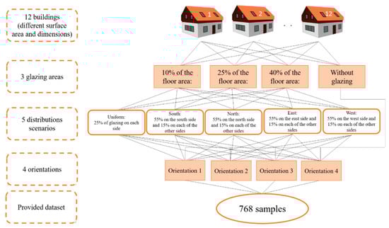
Figure 1.
Graphical view of data preparation.
- (a)
- Uniform: 25% glazing of each of the faces;
- (b)
- East: 55% of the east + 15% of each remaining face;
- (c)
- North: 55% of the north + 15% of each remaining face;
- (d)
- West: 55% of the west + 15% of each remaining face;
- (e)
- South: 55% of the south + 15% of each remaining face.
3. Methodology
This subsection presents the enhancement and construction of the new model. The following topics are discussed in this subsection: (1) ANFIS and (2) teaching–learning based optimization (TLBO).
3.1. Adaptive Neuro–Fuzzy Interface System (ANFIS)
In recent years, researchers have paid much attention to the fuzzy theory, which is ascribable to its capability of illustrating complicated procedures using the if–then rules and concepts [65]. The source of inspiration for the fuzzy theory is the decision-making concept in human life [66]. Nonetheless, it is noteworthy that this algorithm does not present preferred results for unanticipated circumstances [67]. Therefore, in order to reach the self-learning feature, an artificial neural network (ANN) [68,69] has been used for the optimization of the fuzzy theory as an adaptive neuro–fuzzy interface system [70,71]. Jang [72] has suggested an adaptive neuro–fuzzy interface system as a combination of a fuzzy system and an artificial neural network. It is noteworthy that the adaptive neuro–fuzzy interface system presents better results in comparison with a fuzzy inference system (FIS) when solving nonlinear problems. In accordance with the adaptive neuro–fuzzy interface system, a fuzzy inference system is used for training of a multilayer network [73]. By combining backpropagation gradient descent and least-squares techniques, the parameters of the membership function (MF) of the fuzzy inference system can be trained by training the input data through the adaptive neuro–fuzzy interface system. The layers in the ANFIS model are of the following structure [74]:
The adaptive nodes contained in each node in layer 1 are:
in which y and x stand for the input nodes. B and A stand for the linguistic variables, and and indicate the membership functions of the suggested node. In the second layer, the output of each node is expressed by Equation (3), that is the output of the whole signals of input to the suggested node [75].
in which stands for the output of each node.
The normalized outcome of the second layer is regarded as the third layer’s nodes.
A function of a node is utilized for the layer 4 in order to associate each node as below:
in which stands for the normalized the firepower of the third layer, and , , and represent the parameters of the node. The parameters in layer 4 are regarded as parameters of the result.
The summation of the entire signals of the input is regarded as a single node of the fifth layer.
3.2. Teaching–Learning Based Optimization (TLBO)
The teaching–learning based optimization algorithm (TLBO), which was presented by Rao et al. [76,77,78], is an algorithm inspired by the teaching–learning procedure. TLBO acts on the basis of the effect of a teacher’s influence on the learners’ output in a class [79]. This algorithm imitates the teaching–learning capability of learners and a teacher in a classroom [80]. The two key elements of the algorithm are learners and a teacher [81]. The algorithm expresses two basic learning modes: learning from a teacher (called the teacher phase) and learning through interactions with other learners (called the learner phase). The output of the teaching–learning based optimization algorithm is the learners’ grades or results, which are dependent on the teacher’s quality. As a result, the teacher is generally regarded as a highly educated individual who attempts to train learners so that they become capable of obtaining better results with respect to their grades or marks. Furthermore, learners can additionally learn from the interactions amongst themselves, which is also helpful in the improvement of their results.
Teaching–learning based optimization is a population-based technique. A group of learners is regarded as the population in the TLBO algorithm, and various design variables are regarded as various subjects presented to the learners, and the result of the learners is similar to the ‘fitness’ value of the optimization problem. The best solution available among the whole population is regarded as the teacher. The work of teaching–learning based optimization is dividable into two parts of the ‘Learner’ and the ‘Teacher’ stages.
The tasks of both stages are expressed as follows.
- (a)
- Teacher stage
This is the first stage of the TLBO algorithm in which learners are trained by the teacher. In the course of the same phase, the teacher aims to improve the mean result of the classroom from any value to his/her own level (i.e., ). However, this is impossible in practice, and depending on his/her capabilities, a teacher is capable of moving the mean of the classroom to any other value , which is better than . If stands for the mean and represents the teacher at any iteration i, will endeavor to enhance the existing mean toward it. Thus, the new mean will be designated as , and the difference between the new mean and the current mean is expressed by the following equation [78].
in which represents the random number within the [0,1] range, and stands for the teaching factor that determines the value of the mean to be changed. can adopt a value of 2 or 1, which is a heuristic step decided in a random manner with equal probability as:
The teaching factor is randomly created in the course of the algorithm execution within the 1–2 range, where 1 indicates no advancement in the knowledge level, while 2 means the complete knowledge transfer. Thus, the in-between values reflect the knowledge transfer level, which may assume any value depending on the capabilities of the learner. The attempts in this study were made by considering the values within the 1–2 range; however, no improvement was observed in the results. As a result, to streamline the network, it is proposed that the factor of teaching may assume either value of 2 or 1 according to the rounding-up criteria. Nonetheless, any value of within the 1–2 range can be considered.
On the basis of the same Difference_Mean, the current solution is updated in accordance with the following equation:
- (b)
- Learner stage
The second stage of the TLBO algorithm is the learner stage, in which the learners’ wisdom is increased through the interactions among themselves. In order to improve his/her knowledge, a learner interacts with other learners randomly, and if the knowledge of the other learner is more than him/her, the learner learns new things. One can mathematically express the learning phenomenon of this phase as below.
Considering two different learners and , where i ≠ j, at any given iteration i,
If presents a better function value, accept it. One can summarize the implementation steps of the teaching–learning based optimization as the following:
Step 1: Through random generation, initialize design variables of the optimization problem and the population (namely, learners) and then estimate them.
Step 2: Consider the best learner in each subject as a teacher for the same subject. Then, compute the learners’ mean result in each subject.
Step 3: Determine the discrepancy between the best mean result and the present mean result in accordance with Equation (7) using the teaching factor ().
Step 4: Upgrade the wisdom of learners with the help of the teacher’s wisdom in accordance with Equation (9).
Step 5: Upgrade the wisdom of learners using the wisdom of another learner in accordance with Equations (10) and (11).
Step 6: Repeat the process from steps 2 to 5 until meeting the termination criterion.
4. Results and Discussion
In accordance with Section 1, the present paper studies the capabilities of a novel optimization algorithm based on the ANFIS network for approximation of heating load using the MATLAB programming software package (version 14.0). Such an objective is satisfied through the synthesis of the algorithms using an adaptive neuro–fuzzy interface system. Thanks to a particular search scheme, the algorithm is aimed at finding the most suitable values for the computed weights pertaining to the adaptive neuro–fuzzy interface system. Particularly, in order to generate the spatial database, eight HL factors were considered (i.e., surface area, relative compactness, roof area, wall area, orientation, overall height, glazing area distribution, and glazing area). In addition, while 80% of the dataset was assigned to the training procedure, the extant 20% was allocated to the validation process of the performance of the TLBO–ANFIS model.
4.1. Accuracy Indexes
The mean absolute error (MAE) and root mean square error (RMSE) are described to measure the prediction and learning errors. MAE and RMSE formulations are presented by Equations (12) and (13). In addition, Equation (14) defines the coefficient of determination (R2), which is employed for the calculation of the compatibility between the predicted and measured heating loads [63]:
In these equations, and stand for the predicted and measured heating loads, respectively. In addition, represents the average of the observed heating loads, and U stands for the number of records.
4.2. Incorporated FIS with Optimizers
An ensemble of TLBO–ANFIS is generated as soon as the metaheuristic algorithms are synthesized with the adaptive neuro–fuzzy interface system. The training samples feed such an ensemble in order to validate the dependency between the heating load and its associated parameters. Considering the optimization performance of the models, a number of 1000 iterations are carried out for the model in order to complete the process of optimization. In order to report the objective function, the root mean square error of the results is determined at each repetition. It is noteworthy that given that this stage is allocated to pattern recognition, the root mean square error of the training data is reported.
One of the key factors in the TLBO–ANFIS algorithm is the number of the concerned population. The present study has tested a number of ten different population sizes (50–500) for the model, among which the size giving the minimum RMSE is chosen as the optimum complexity. Figure 2 shows the root mean square errors. In accordance with the figure, the minimum value of RMSE (2.3838) is obtained for a population of 50 for the TLBO–ANFIS.
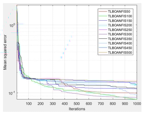
Figure 2.
Alteration of MSE versus iterations for the TLBO–ANFIS.
The rank analysis concept has been adopted from a study by Zhang et al. [82]. This method allocated the best rank to a method with the highest value for each index, whereas a rank of 1 was allocated to the method with the worst value, singly for the testing and training outputs. Then, by summation of their ranks, the total score was estimated. Eventually, by summation of the ranks of the testing and training stages, the final score was estimated for each model.
The ranking system developed on the basis of the estimated values for RMSE and R2 is reported in Table 2. As the table shows, a total ranking score (TRS) is obtained for each population size of the predictive model, which indicates the final rank for each population size. In this regard, a total score of 40 obtained for a population size of 100 in the TLBO–ANFIS technique indicates that the combination of the ANFIS and TLBO algorithm brings about a high accuracy technique for the prediction of HL. According to the results, the combination of the evolutionary algorithm and the employed fuzzy-based tool shows efficient performance for HL prediction purposes. Moreover, given the high-speed convergence of the TLBO–ANFIS, one can mention the speed of this model as its advantage over the alternative statistical-based and intelligent techniques.
Table 2.
Obtained results for the TLBO–ANFIS having different population sizes.
To anticipate the HL, two advanced computational techniques are developed. First, the model is trained using the training data. The performance of the developed model in the prediction of HL on the basis of the variables affecting the testing and training datasets of buildings is shown in Figure 3.
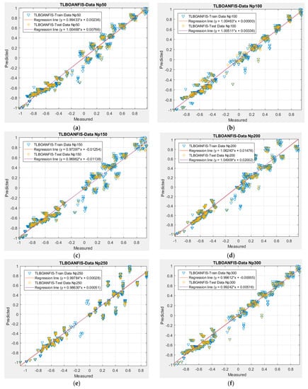
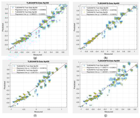
Figure 3.
The accuracy performance of testing and training dataset for TLBO–ANFIS. (a) TLBO–ANFIS Np = 50; (b) TLBO–ANFIS Np = 100; (c) TLBO–ANFIS Np = 150; (d) TLBO–ANFIS Np = 200; (e) TLBO–ANFIS Np = 250; (f) TLBO–ANFIS Np = 300; (g) TLBO–ANFIS Np = 350; (h) TLBO–ANFIS Np = 400; (i) TLBO–ANFIS Np = 450; (j) TLBO–ANFIS Np = 500.
At the same time, the values obtained for R2 show a consistency higher than 96% for the output and target heating loads. In addition, the calculated training R2s (0.98356, 0.98931, 0.97845, 0.9734, 0.96497, 0.98773, 0.97708, 0.9856, 0.9739, and 0.96405) and testing R2s (0.98525, 0.98933, 0.98136, 0.97391, 0.9666, 0.98772, 0.98064, 0.9874, 0.97597, and 0.9627) for ten population sizes of 50, 100, 150, 200, 250, 300, 350, 400, 450, and 500, respectively, present a high accuracy in HL prediction.
This section compares the outputs (namely, the anticipated heating loads) with the target values (namely, the measured heating loads) in order to evaluate the performance of the applied model. Figure 4, Figure 5, Figure 6, Figure 7 and Figure 8 present the results of the testing and training phases and the difference between each set of the target and output heating loads. For the training phase, the acquired error values are within the [−0.0005572, 0.079956], [0.0067801, 0.12941], [0.00041716, 0.085609], [−0.0060323, 0.092914], and [0.024064, 0.1464] range for the predictions of the TLBO–ANFIS for five population sizes of 100, 200, 300, 400, and 500, respectively.
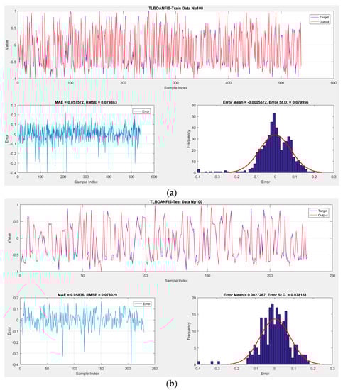
Figure 4.
Error value and Frequency in TLBO–ANFIS-100 best fit structure. (a) Training dataset; (b) Testing dataset.
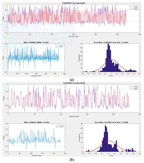
Figure 5.
Error value and Frequency in TLBO–ANFIS-200 best fit structure. (a) Training dataset; (b) Testing dataset.
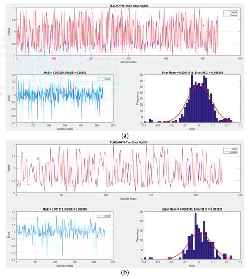
Figure 6.
Error value and Frequency in TLBO–ANFIS-300 best fit structure. (a) Training dataset; (b) Testing dataset.
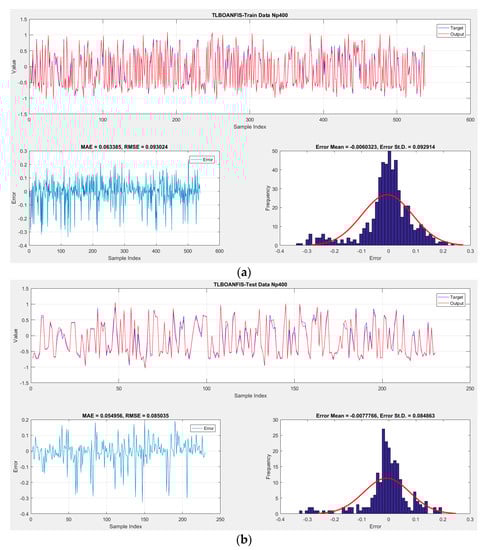
Figure 7.
Error value and Frequency in TLBO–ANFIS-400 best fit structure. (a) Training dataset; (b) Testing dataset.
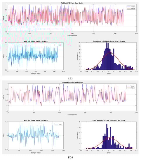
Figure 8.
Error value and frequency in TLBO–ANFIS-500 best fit structure. (a) Training dataset; (b) Testing dataset.
As stated in the previous section, the values of root–mean–square error for the training are 0.07948, 0.12544, 0.0855, 0.09258, and 0.14549 for the five population sizes of 100, 200, 300, 400, and 500, respectively. In addition, the calculated MAEs (0.057572, 0.088625, 0.063508, 0.063385, and 0.10723) indicate a low value of training error for all swarm sizes.
In the testing phase, the RMSEs (0.07794, 0.12137, 0.08355, 0.08464, and 0.14471) demonstrate that the weights (and biases) tuned via the TLBO algorithm are capable of constructing an ANFIS. In addition, the mean absolute errors of 0.05836, 0.086274, 0.061333, 0.054956, and 0.10469 show a reasonable generalization error for all five population sizes.
5. Discussion
Generally speaking, a great number of engineering measurements have approved the superiority of intelligent models over experimental and traditional techniques. Besides the satisfactory accuracy of these models, one of the deterministic benefits of their application is their ease of implementation. For instance, when analyzing the energy efficiency, some drawbacks may remain, which are related to the use of forward modeling techniques (poor capability for buildings with residents [37]) and commonly used simulation packages (varying simulation accuracies [38]). As a result, indirect evaluative models, in particular the models provided by the present paper, are more satisfactory compared to destructive and costly approaches [83]. This issue is more emphasized when an optimum methodology is presented using metaheuristic approaches [84,85,86]. To put it another way, the application of optimization algorithms constructs the ensembles capable of operating at optimal conditions [87].
From the practical viewpoint, their application is definable for the presented methodologies. We can refer to the following two examples:
(a) For the upcoming construction projects, the models presented above are capable of providing accurate early measurements of the necessary TL with regard to the building specifications and dimensions. Such models can provide the owners and engineers with effective assistance in the provision of appropriate heating, ventilating, and air conditioning systems.
(b) An alternative form of early-stage assistance in reconstruction projects could be the appropriate building design and modifying its network via the input variables (RC, RA, WA, GA, SA, OH, GAD, and OR). In this regard, one can study the result of input parameters independently in order to understand the thermal behavior. Nonetheless, the TLBO–ANFIS can predict it satisfactorily. As a result, such an algorithm is also capable of providing reliable estimations for buildings.
In this sense, it is also noteworthy that the presented model was provided as an explicit mathematical expression, which is used more conveniently in comparison with the GUI form in MATLAB.
In spite of a variety of advantages provided after solving an optimization problem, it is necessary to spend an adequate period of time on finding a global solution. As a result, keeping a balance between the model accuracy and time effectiveness can affect the selection of the most effective model. Nonetheless, according to the belief of authors, conducting feature validity analysis and also setting the hyper-parameters of the optimizers appropriately may create a less sophisticated problem space and, thereby, result in more efficient solutions. Results show that the teaching–learning based optimization algorithm combined with ANFIS is the model with high accuracy (Figure 2, Figure 3, Figure 4, Figure 5, Figure 6, Figure 7 and Figure 8). This entails choosing a suitable methodology with regard to both accuracy and time. For instance, in projects in which time is not a priority, it is reasonable to use the most accurate mode (namely, it does not matter how time-consuming it is); however, for time-sensitive purposes, one can allow tolerance for the accuracy in order to find a faster solution. Nonetheless, it is noteworthy that, in general, the models were not much different in terms of their performance, and all of them could be appropriately used for practical applications.
6. Conclusions
New models have been developed in recent years in order to present an accurate estimation of the energy consumption of buildings. A fuzzy algorithm was utilized in the present paper in order to eliminate the drawbacks associated with the backpropagation algorithms. In this regard, through teaching–learning based optimization (TLBO), a typical adaptive neuro–fuzzy interface system (ANFIS) was synthesized (TLBO–ANFIS) in order to predict the heating load (HL) of an occupied residential building. For the same purpose, eight influential energy parameters, i.e., surface area, relative compactness, area of the wall, area of the roof, orientation, overall height, glazing area distribution, and area of glazing, were included as the inputs of the developed networks. Given the four glazing areas, twelve buildings, four orientations, and five distribution modes, 768 scenarios were analyzed and modeled within the Ecotect environment. While 80% (614 records) of the dataset was allocated to the TLBO–ANFIS model, their efficiency was estimated using the remaining 20%. The suggested model is used in its optimum circumstances, and in order to estimate the accuracy of each technique, three recognized statistical indices, i.e., mean absolute error (MAE), the coefficient of determination (R2), and root mean square error (RMSE), were used. The following results were obtained in the present research:
The estimated R2 for both testing and training (0.98933, 0.98931) phases indicated that TLBO helps the ANFIS to enhance the accuracy of the results, and a high value of R2 indicates the high accuracy of this model in forecasting the heating load.
According to the estimated root mean square error, the training error of TLBO–ANFIS was 0.07984 and 0.07794 in the training and testing stages, respectively. Considering the low value of RMSE, it can be concluded that the TLBO–ANFIS model is suitable for the estimation of the heating load in residential buildings.
Author Contributions
L.K.F.: methodology, software. B.N.L.: writing, software. All authors have read and agreed to the published version of the manuscript.
Funding
This research received no external funding.
Data Availability Statement
The data available based on the reader’s request.
Conflicts of Interest
The authors declare no conflict of interest.
Abbreviations
| TLBO | Teaching–learning based Optimization |
| ANFIS | adaptive neuro–fuzzy interface system |
| HL | Heating Load |
| R2 | Coefficient of Determination |
| RMSE | Root Mean Squared Error |
| MAE | Mean Average Error |
| HVAC | heating, ventilating, and air conditioning |
References
- Shi, X.; Tian, Z.; Chen, W.; Si, B.; Jin, X. A review on building energy efficient design optimization rom the perspective of architects. Renew. Sustain. Energy Rev. 2016, 65, 872–884. [Google Scholar] [CrossRef]
- Roy, S.S.; Samui, P.; Nagtode, I.; Jain, H.; Shivaramakrishnan, V.; Mohammadi-Ivatloo, B. Forecasting heating and cooling loads of buildings: A comparative performance analysis. J. Ambient Intell. Humaniz. Comput. 2020, 11, 1253–1264. [Google Scholar] [CrossRef]
- Zhou, G.; Moayedi, H.; Bahiraei, M.; Lyu, Z. Employing artificial bee colony and particle swarm techniques for optimizing a neural network in prediction of heating and cooling loads of residential buildings. J. Clean. Prod. 2020, 254, 120082. [Google Scholar] [CrossRef]
- Liu, K.; Yang, Z.; Wei, W.; Gao, B.; Xin, D.; Sun, C.; Gao, G.; Wu, G. Novel detection approach for thermal defects: Study on its feasibility and application to vehicle cables. High Volt. 2022, 1–10. [Google Scholar] [CrossRef]
- Mou, J.; Duan, P.; Gao, L.; Liu, X.; Li, J. An effective hybrid collaborative algorithm for energy-efficient distributed permutation flow-shop inverse scheduling. Future Gener. Comput. Syst. 2022, 128, 521–537. [Google Scholar] [CrossRef]
- Zaman, K.; Shahbaz, M.; Loganathan, N.; Raza, S.A. Tourism development, energy consumption and Environmental Kuznets Curve: Trivariate analysis in the panel of developed and developing countries. Tour. Manag. 2016, 54, 275–283. [Google Scholar] [CrossRef]
- Rashid, A.S.A.; Kalatehjari, R.; Noor, N.M.; Yaacob, H.; Moayedi, H.; Sing, L.K. Relationship between liquidity index and stabilized strength of local subgrade materials in a tropical area. Measurement 2014, 55, 231–237. [Google Scholar] [CrossRef]
- McQuiston, F.C.; Parker, J.D.; Spitler, J.D. Heating, Ventilating, and Air Conditioning: Analysis and Design; John Wiley & Sons: Hoboken, NJ, USA, 2004. [Google Scholar]
- Huang, Y.; Li, C. Accurate heating, ventilation and air conditioning system load prediction for residential buildings using improved ant colony optimization and wavelet neural network. J. Build. Eng. 2021, 35, 101972. [Google Scholar] [CrossRef]
- Sarihi, S.; Saradj, F.M.; Faizi, M. A critical review of façade retrofit measures for minimizing heating and cooling demand in existing buildings. Sustain. Cities Soc. 2021, 64, 102525. [Google Scholar] [CrossRef]
- Ihara, T.; Gustavsen, A.; Jelle, B.P. Effect of facade components on energy efficiency in office buildings. Appl. Energy 2015, 158, 422–432. [Google Scholar] [CrossRef]
- Knight, D.; Roth, S.; Rosen, S.L. Using BIM in HVAC design. Ashrae J. 2010, 52, 24–29. [Google Scholar]
- Ikeda, S.; Ooka, R. Metaheuristic optimization methods for a comprehensive operating schedule of battery, thermal energy storage, and heat source in a building energy system. Appl. Energy 2015, 151, 192–205. [Google Scholar] [CrossRef]
- Sonmez, Y.; Guvenc, U.; Kahraman, H.T.; Yilmaz, C. A comperative study on novel machine learning algorithms for estimation of energy performance of residential buildings. In Proceedings of the 2015 3rd International Istanbul Smart Grid Congress and Fair (ICSG), Istanbul, Turkey, 29–30 April 2015; pp. 1–7. [Google Scholar]
- Ozarisoy, B. Energy effectiveness of passive cooling design strategies to reduce the impact of long-term heatwaves on occupants’ thermal comfort in Europe: Climate change and mitigation. J. Clean. Prod. 2022, 330, 129675. [Google Scholar] [CrossRef]
- Moayedi, H.; Mu’azu, M.A.; Foong, L.K. Novel swarm-based approach for predicting the cooling load of residential buildings based on social behavior of elephant herds. Energy Build. 2020, 206, 109579. [Google Scholar] [CrossRef]
- Sadeghian, O.; Moradzadeh, A.; Mohammadi-Ivatloo, B.; Abapour, M.; Anvari-Moghaddam, A.; Lim, J.S.; Marquez, F.P.G. A comprehensive review on energy saving options and saving potential in low voltage electricity distribution networks: Building and public lighting. Sustain. Cities Soc. 2021, 72, 103064. [Google Scholar] [CrossRef]
- Mustafaraj, G.; Marini, D.; Costa, A.; Keane, M. Model calibration for building energy efficiency simulation. Appl. Energy 2014, 130, 72–85. [Google Scholar] [CrossRef]
- Sohani, A.; Rezapour, S.; Sayyaadi, H. Comprehensive performance evaluation and demands’ sensitivity analysis of different optimum sizing strategies for a combined cooling, heating, and power system. J. Clean. Prod. 2021, 279, 123225. [Google Scholar] [CrossRef]
- Zhao, Y.; Joseph, A.J.J.M.; Zhang, Z.; Ma, C.; Gul, D.; Schellenberg, A.; Hu, N. Deterministic snap-through buckling and energy trapping in axially-loaded notched strips for compliant building blocks. Smart Mater. Struct. 2020, 29, 02LT03. [Google Scholar] [CrossRef]
- Zhao, Y.; Hu, H.; Bai, L.; Tang, M.; Chen, H.; Su, D. Fragility analyses of bridge structures using the logarithmic piecewise function-based probabilistic seismic demand model. Sustainability 2021, 13, 7814. [Google Scholar] [CrossRef]
- Yan, B.; Ma, C.; Zhao, Y.; Hu, N.; Guo, L. Geometrically Enabled Soft Electroactuators via Laser Cutting. Adv. Eng. Mater. 2019, 21, 1900664. [Google Scholar] [CrossRef]
- Alnaqi, A.A.; Moayedi, H.; Shahsavar, A.; Nguyen, T.K. Prediction of energetic performance of a building integrated photovoltaic/thermal system thorough artificial neural network and hybrid particle swarm optimization models. Energy Convers. Manag. 2019, 183, 137–148. [Google Scholar] [CrossRef]
- Yu, D.; Wu, J.; Wang, W.; Gu, B. Optimal performance of hybrid energy system in the presence of electrical and heat storage systems under uncertainties using stochastic p-robust optimization technique. Sustain. Cities Soc. 2022, 83, 103935. [Google Scholar] [CrossRef]
- Tien Bui, D.; Moayedi, H.; Anastasios, D.; Kok Foong, L. Predicting heating and cooling loads in energy-efficient buildings using two hybrid intelligent models. Appl. Sci. 2019, 9, 3543. [Google Scholar] [CrossRef]
- Nguyen, H.; Moayedi, H.; Jusoh, W.A.W.; Sharifi, A. Proposing a novel predictive technique using M5Rules-PSO model estimating cooling load in energy-efficient building system. Eng. Comput. 2020, 36, 857–866. [Google Scholar] [CrossRef]
- Fang, J.; Kong, G.; Yang, Q. Group Performance of Energy Piles under Cyclic and Variable Thermal Loading. J. Geotech. Geoenvironmental Eng. 2022, 148, 04022060. [Google Scholar] [CrossRef]
- Heydari, A.; Sadati, S.E.; Gharib, M.R. Effects of different window configurations on energy consumption in building: Optimization and economic analysis. J. Build. Eng. 2021, 35, 102099. [Google Scholar] [CrossRef]
- Moayedi, H.; Mosavi, A. Double-target based neural networks in predicting energy consumption in residential buildings. Energies 2021, 14, 1331. [Google Scholar] [CrossRef]
- Fanti, M.P.; Mangini, A.M.; Roccotelli, M. A simulation and control model for building energy management. Control Eng. Pract. 2018, 72, 192–205. [Google Scholar] [CrossRef]
- Egan, J.; Finn, D.; Soares, P.H.D.; Baumann, V.A.R.; Aghamolaei, R.; Beagon, P.; Neu, O.; Pallonetto, F.; O’Donnell, J. Definition of a useful minimal-set of accurately-specified input data for Building Energy Performance Simulation. Energy Build. 2018, 165, 172–183. [Google Scholar] [CrossRef]
- Moayedi, H.; Mosavi, A. An innovative metaheuristic strategy for solar energy management through a neural networks framework. Energies 2021, 14, 1196. [Google Scholar] [CrossRef]
- Zhao, H.-x.; Magoulès, F. A review on the prediction of building energy consumption. Renew. Sustain. Energy Rev. 2012, 16, 3586–3592. [Google Scholar] [CrossRef]
- Li, H.; Hou, K.; Xu, X.; Jia, H.; Zhu, L.; Mu, Y. Probabilistic energy flow calculation for regional integrated energy system considering cross-system failures. Appl. Energy 2022, 308, 118326. [Google Scholar] [CrossRef]
- Nazari, S.; Bahiraei, M.; Moayedi, H.; Safarzadeh, H. A proper model to predict energy efficiency, exergy efficiency, and water productivity of a solar still via optimized neural network. J. Clean. Prod. 2020, 277, 123232. [Google Scholar] [CrossRef]
- Moayedi, H.; Nazir, R.; Gör, M.; Kassim, K.A.; Foong, L.K. A new real-time monitoring technique in calculation of the py curve of single thin steel piles considering the influence of driven energy and using strain gauge sensors. Measurement 2020, 153, 107365. [Google Scholar] [CrossRef]
- Park, J.; Lee, S.J.; Kim, K.H.; Kwon, K.W.; Jeong, J.-W. Estimating thermal performance and energy saving potential of residential buildings using utility bills. Energy Build. 2016, 110, 23–30. [Google Scholar] [CrossRef]
- Yezioro, A.; Dong, B.; Leite, F. An applied artificial intelligence approach towards assessing building performance simulation tools. Energy Build. 2008, 40, 612–620. [Google Scholar] [CrossRef]
- York, D.; Cappiello, C.; Olson, K. DOE-2 Reference Manual: Version 2.1 C; Los Alamos National Laboratory, Solar Energy Group: Los Alamos, NM, USA, 1984. [Google Scholar]
- Crawley, D.B.; Lawrie, L.K.; Winkelmann, F.C.; Buhl, W.F.; Huang, Y.J.; Pedersen, C.O.; Strand, R.K.; Liesen, R.J.; Fisher, D.E.; Witte, M.J. EnergyPlus: Creating a new-generation building energy simulation program. Energy Build. 2001, 33, 319–331. [Google Scholar] [CrossRef]
- Yan, D.; Xia, J.; Tang, W.; Song, F.; Zhang, X.; Jiang, Y. DeST—An integrated building simulation toolkit Part I: Fundamentals. Build. Simul. 2008, 1, 95–110. [Google Scholar] [CrossRef]
- O’Neill, Z.; O’Neill, C. Development of a probabilistic graphical model for predicting building energy performance. Appl. Energy 2016, 164, 650–658. [Google Scholar] [CrossRef]
- Catalina, T.; Virgone, J.; Blanco, E. Development and validation of regression models to predict monthly heating demand for residential buildings. Energy Build. 2008, 40, 1825–1832. [Google Scholar] [CrossRef]
- Yu, Z.; Haghighat, F.; Fung, B.C.; Yoshino, H. A decision tree method for building energy demand modeling. Energy Build. 2010, 42, 1637–1646. [Google Scholar] [CrossRef]
- Adedeji, P.A.; Akinlabi, S.; Madushele, N.; Olatunji, O.O. Hybrid adaptive neuro-fuzzy inference system (ANFIS) for a multi-campus university energy consumption forecast. Int. J. Ambient Energy 2022, 43, 1685–1694. [Google Scholar] [CrossRef]
- Moayedi, H.; Varamini, N.; Mosallanezhad, M.; Foong, L.K. Applicability and comparison of four nature-inspired hybrid techniques in predicting driven piles’ friction capacity. Transp. Geotech. 2022, 37, 100875. [Google Scholar] [CrossRef]
- Osouli, A.; Ebrahimi, M.; Alzamora, D.; Shoup, H.Z.; Pagenkopf, J. Multi-Criteria Assessment of Bridge Sites for Conducting PSTD/ISTD: Case Histories. Transp. Res. Rec. 2022. [Google Scholar] [CrossRef]
- Wu, P.; Liu, A.; Fu, J.; Ye, X.; Zhao, Y. Autonomous surface crack identification of concrete structures based on an improved one-stage object detection algorithm. Eng. Struct. 2022, 272, 114962. [Google Scholar] [CrossRef]
- Shahsavar, A.; Moayedi, H.; Al-Waeli, A.H.; Sopian, K.; Chelvanathan, P. Machine learning predictive models for optimal design of building-integrated photovoltaic-thermal collectors. Int. J. Energy Res. 2020, 44, 5675–5695. [Google Scholar] [CrossRef]
- Davidson, C.; Brown, M.J.; Cerfontaine, B.; Al-Baghdadi, T.; Knappett, J.; Brennan, A.; Augarde, C.; Coombs, W.; Wang, L.; Blake, A.; et al. Physical modelling to demonstrate the feasibility of screw piles for offshore jacket-supported wind energy structures. Geotechnique 2022, 72, 108–126. [Google Scholar] [CrossRef]
- Lu, C.; Liu, Q.; Zhang, B.; Yin, L. A Pareto-based hybrid iterated greedy algorithm for energy-efficient scheduling of distributed hybrid flowshop. Expert Syst. Appl. 2022, 204, 117555. [Google Scholar] [CrossRef]
- Zhao, Y.; Yan, Q.; Yang, Z.; Yu, X.; Jia, B. A novel artificial bee colony algorithm for structural damage detection. Adv. Civ. Eng. 2020, 2020, 3743089. [Google Scholar] [CrossRef]
- Gao, W.; Alsarraf, J.; Moayedi, H.; Shahsavar, A.; Nguyen, H. Comprehensive preference learning and feature validity for designing energy-efficient residential buildings using machine learning paradigms. Appl. Soft Comput. 2019, 84, 105748. [Google Scholar] [CrossRef]
- Wang, J.; Qi, X.; Ren, F.; Zhang, G.; Wang, J. Optimal design of hybrid combined cooling, heating and power systems considering the uncertainties of load demands and renewable energy sources. J. Clean. Prod. 2021, 281, 125357. [Google Scholar] [CrossRef]
- Metallidou, C.K.; Psannis, K.E.; Egyptiadou, E.A. Energy efficiency in smart buildings: IoT approaches. IEEE Access 2020, 8, 63679–63699. [Google Scholar] [CrossRef]
- Bui, X.-N.; Moayedi, H.; Rashid, A.S.A. Developing a predictive method based on optimized M5Rules–GA predicting heating load of an energy-efficient building system. Eng. Comput. 2020, 36, 931–940. [Google Scholar] [CrossRef]
- Moayedi, H.; Bui, D.T.; Dounis, A.; Lyu, Z.; Foong, L.K. Predicting heating load in energy-efficient buildings through machine learning techniques. Appl. Sci. 2019, 9, 4338. [Google Scholar] [CrossRef]
- Li, K.; Su, H.; Chu, J. Forecasting building energy consumption using neural networks and hybrid neuro-fuzzy system: A comparative study. Energy Build. 2011, 43, 2893–2899. [Google Scholar] [CrossRef]
- Gao, W.; Moayedi, H.; Shahsavar, A. The feasibility of genetic programming and ANFIS in prediction energetic performance of a building integrated photovoltaic thermal (BIPVT) system. Sol. Energy 2019, 183, 293–305. [Google Scholar] [CrossRef]
- Qiao, W.; Moayedi, H.; Foong, L.K. Nature-inspired hybrid techniques of IWO, DA, ES, GA, and ICA, validated through a k-fold validation process predicting monthly natural gas consumption. Energy Build. 2020, 217, 110023. [Google Scholar] [CrossRef]
- Tsanas, A.; Xifara, A. Accurate quantitative estimation of energy performance of residential buildings using statistical machine learning tools. Energy Build. 2012, 49, 560–567. [Google Scholar] [CrossRef]
- Catalina, T.; Iordache, V.; Caracaleanu, B. Multiple regression model for fast prediction of the heating energy demand. Energy Build. 2013, 57, 302–312. [Google Scholar] [CrossRef]
- Boldina, I.; Beninger, P.G. Strengthening statistical usage in marine ecology: Linear regression. J. Exp. Mar. Biol. Ecol. 2016, 474, 81–91. [Google Scholar] [CrossRef]
- Duarte, G.R.; da Fonseca, L.G.; Goliatt, P.; de Castro Lemonge, A.C. Comparison of machine learning techniques for predicting energy loads in buildings. Ambiente Construído 2017, 17, 103–115. [Google Scholar] [CrossRef]
- Mehrabi, M.; Pradhan, B.; Moayedi, H.; Alamri, A. Optimizing an adaptive neuro-fuzzy inference system for spatial prediction of landslide susceptibility using four state-of-the-art metaheuristic techniques. Sensors 2020, 20, 1723. [Google Scholar] [CrossRef] [PubMed]
- Moayedi, H.; Nguyen, H.; Kok Foong, L. Nonlinear evolutionary swarm intelligence of grasshopper optimization algorithm and gray wolf optimization for weight adjustment of neural network. Eng. Comput. 2021, 37, 1265–1275. [Google Scholar] [CrossRef]
- Dehnavi, A.; Aghdam, I.N.; Pradhan, B.; Varzandeh, M.H.M. A new hybrid model using step-wise weight assessment ratio analysis (SWARA) technique and adaptive neuro-fuzzy inference system (ANFIS) for regional landslide hazard assessment in Iran. Catena 2015, 135, 122–148. [Google Scholar] [CrossRef]
- Mosallanezhad, M.; Moayedi, H. Developing hybrid artificial neural network model for predicting uplift resistance of screw piles. Arab. J. Geosci. 2017, 10, 1–10. [Google Scholar] [CrossRef]
- Moayedi, H.; Gör, M.; Lyu, Z.; Bui, D.T. Herding Behaviors of grasshopper and Harris hawk for hybridizing the neural network in predicting the soil compression coefficient. Measurement 2020, 152, 107389. [Google Scholar] [CrossRef]
- Zhao, Y.; Foong, L.K. Predicting Electrical Power Output of Combined Cycle Power Plants Using a Novel Artificial Neural Network Optimized by Electrostatic Discharge Algorithm. Measurement 2022, 198, 111405. [Google Scholar] [CrossRef]
- Zhao, Y.; Wang, Z. Subset simulation with adaptable intermediate failure probability for robust reliability analysis: An unsupervised learning-based approach. Struct. Multidiscip. Optim. 2022, 65, 1–22. [Google Scholar] [CrossRef]
- Jang, J.-S. ANFIS: Adaptive-network-based fuzzy inference system. IEEE Trans. Syst. Man Cybern. 1993, 23, 665–685. [Google Scholar] [CrossRef]
- Dixon, B. Applicability of neuro-fuzzy techniques in predicting ground-water vulnerability: A GIS-based sensitivity analysis. J. Hydrol. 2005, 309, 17–38. [Google Scholar] [CrossRef]
- Termeh, S.V.R.; Kornejady, A.; Pourghasemi, H.R.; Keesstra, S. Flood susceptibility mapping using novel ensembles of adaptive neuro fuzzy inference system and metaheuristic algorithms. Sci. Total Environ. 2018, 615, 438–451. [Google Scholar] [CrossRef] [PubMed]
- Zhang, W.; Zheng, Z.; Liu, H. A novel droop control method to achieve maximum power output of photovoltaic for parallel inverter system. CSEE J. Power Energy Syst. 2021, 1–9. [Google Scholar] [CrossRef]
- Rao, R.V.; Savsani, V.J.; Vakharia, D. Teaching–learning-based optimization: An optimization method for continuous non-linear large scale problems. Inf. Sci. 2012, 183, 1–15. [Google Scholar] [CrossRef]
- Rao, R.V.; Savsani, V.; Balic, J. Teaching–learning-based optimization algorithm for unconstrained and constrained real-parameter optimization problems. Eng. Optim. 2012, 44, 1447–1462. [Google Scholar] [CrossRef]
- Rao, R.V.; Savsani, V.J.; Vakharia, D. Teaching–learning-based optimization: A novel method for constrained mechanical design optimization problems. Comput.-Aided Des. 2011, 43, 303–315. [Google Scholar] [CrossRef]
- Almutairi, K.; Algarni, S.; Alqahtani, T.; Moayedi, H.; Mosavi, A. A TLBO-Tuned Neural Processor for Predicting Heating Load in Residential Buildings. Sustainability 2022, 14, 5924. [Google Scholar] [CrossRef]
- Zhao, Y.; Moayedi, H.; Bahiraei, M.; Foong, L.K. Employing TLBO and SCE for optimal prediction of the compressive strength of concrete. Smart Struct. Syst. 2020, 26, 753–763. [Google Scholar]
- Zhou, G.; Moayedi, H.; Foong, L.K. Teaching–learning-based metaheuristic scheme for modifying neural computing in appraising energy performance of building. Eng. Comput. 2021, 37, 3037–3048. [Google Scholar] [CrossRef]
- Zhang, H.; Zhou, J.; Jahed Armaghani, D.; Tahir, M.; Pham, B.T.; Huynh, V.V. A combination of feature selection and random forest techniques to solve a problem related to blast-induced ground vibration. Appl. Sci. 2020, 10, 869. [Google Scholar] [CrossRef]
- Bui, D.T.; Moayedi, H.; Kalantar, B.; Osouli, A.; Pradhan, B.; Nguyen, H.; Rashid, A.S.A. A novel swarm intelligence—Harris hawks optimization for spatial assessment of landslide susceptibility. Sensors 2019, 19, 3590. [Google Scholar] [CrossRef]
- Zhao, Y.; Hu, H.; Song, C.; Wang, Z. Predicting compressive strength of manufactured-sand concrete using conventional and metaheuristic-tuned artificial neural network. Measurement 2022, 194, 110993. [Google Scholar] [CrossRef]
- Foong, L.K.; Zhao, Y.; Bai, C.; Xu, C. Efficient metaheuristic-retrofitted techniques for concrete slump simulation. Smart Struct. Syst. Int. J. 2021, 27, 745–759. [Google Scholar]
- Huang, X.X.; Moayedi, H.; Gong, S.; Gao, W. Application of metaheuristic algorithms for pressure analysis of crude oil pipeline. Energy Sources Part A Recovery Util. Environ. Eff. 2022, 44, 5124–5142. [Google Scholar] [CrossRef]
- Zhao, Y.; Zhong, X.; Foong, L.K. Predicting the splitting tensile strength of concrete using an equilibrium optimization model. Steel Compos. Struct. Int. J. 2021, 39, 81–93. [Google Scholar]


Publisher’s Note: MDPI stays neutral with regard to jurisdictional claims in published maps and institutional affiliations. |
© 2022 by the authors. Licensee MDPI, Basel, Switzerland. This article is an open access article distributed under the terms and conditions of the Creative Commons Attribution (CC BY) license (https://creativecommons.org/licenses/by/4.0/).