Abstract
Thermal bridges may have a significant prejudicial impact on the thermal behavior and energy efficiency of buildings. Given the high thermal conductivity of steel, in Lightweight Steel Framed (LSF) buildings, this detrimental effect could be even greater. The use of thermal break (TB) strips is one of the most broadly implemented thermal bridge mitigation technics. In a previous study, the performance of TB strips in partition LSF walls was evaluated. However, a search of the literature found no similar experimental campaigns for facade LSF walls, which are even more relevant for a building’s overall energy efficiency since they are in direct contact with the external environmental conditions. In this article the thermal performance of ten facade LSF wall configurations were measured, using the heat flow meter (HFM) method. These measurements were compared to numerical simulation predictions, exhibiting excellent similarity and, consequently, high reliability. One reference wall, three TB strip locations in the steel stud flanges and three TB strip materials were assessed. The outer and inner TB strips showed quite similar thermal performances, but with slightly higher thermal resistance for outer TB strips (around +1%). Furthermore, the TB strips were clearly less efficient in facade LSF walls when compared to their thermal performance improvement in load-bearing partition LSF walls.
1. Introduction
Overall, buildings are responsible for about 36% of global CO2 emissions, making them a key player in the fight against global warming and climate change [1]. The European Union spends approximately 40% of final energy consumption on heating and cooling buildings [2]. For this reason, in recent decades European legislation has been geared towards transforming the existing building stock into a network of nearly zero energy buildings (NZEB) [2], promoting the use of renewable energies and developing renovation strategies to improve the energy efficiency of existing buildings [3].
Currently, approximately 35% of the building stock in the European Union is over 50 years old and needs rehabilitation to meet current energy requirements [4]. Consequently, the European Green Deal presented by the Commission on 11 December 2019 [5], sets out the arrangements for achieving an efficient use of energy and building resources to double the annual renovation rate of the building stock [6]. In line with this initiative, it has been noted that it is important to conduct studies that allow for a reliable thermal characterization of buildings and an exhaustive analysis of the components that make up their envelope [7].
As an alternative for the energy rehabilitation of existing building facades, systems such as External Thermal Insulation Composite Systems (ETICS) have been developed in recent decades [8,9]. These are construction systems that consist of a thermal insulation material applied to the building facade with the help of an adhesive and/or mechanical fastening, and then a reduced thickness rendering system that incorporates a reinforcing mesh [10]. These construction systems make it possible to reduce thermal bridges and moisture condensation on the inside surface of the envelopes, as well as offering the advantage of not reducing the interior space of the rooms in the dwellings and improving the aesthetics of the refurbished facade [11]. Moreover, there are several studies that have found the use of this type of insulation system from the outside saves up to 8% more energy on average than in the case of using an insulation system from the inside [12].
ETICS are also very widely used in Lightweight Steel Framed (LSF) facade walls [13], having the advantage of mitigating the thermal bridges originated by the high thermal conductivity of the steel studs since they are a continuous insulation. There are several types of thermal bridges [13], which could be designated as: (1) repeating thermal bridges (e.g., due to the vertical steel studs inside an LSF wall), where their effect is usually considered by reducing the R-value (increase the U-value); (2) non-repeating (or linear) thermal bridges (e.g., along a wall corner, or along a wall–window joint perimeter [14]), quantified using the linear thermal transmittance (Ψ); and (3) punctual thermal bridges (e.g., due to mechanical steel fasteners crossing the ETICS insulation layer), which are taken into account using the point thermal transmittance (χ). In this study, only the above-mentioned first type of thermal bridges are considered.
The LSF construction system has been used in the last decades due to its multiple advantages such as its low weight compared to its high mechanical resistance [15], a great speed of execution and ease of transport to the building site [16], a high potential for recycling and a high quality as very precise tolerances are achieved in the execution of prefabricated elements [17,18].
However, the existence of thermal bridges through the steel and the lower thermal inertia of the LSF walls can cause problems related to comfort and a higher energy demand [19], with the thermal bridges issue being even more relevant in cold climates [20]. Furthermore, it is sometimes difficult to accurately evaluate the final thermal resistance of the facade as there is a strong contrast between the high thermal conductivity of the steel frame and the insulation materials filling the air cavity [21,22]. Additionally, the size and shape of the stud flanges may have a relevant influence on the thermal performance of LSF walls [23]. Furthermore, the position of the thermal insulation is very important with regards to their effectiveness [24], and the usual fibrous cavity insulation (e.g., mineral wool) is likewise relevant for the noise insulation performance of LSF facade walls [25].
Given the absence of a continuous insulation layer, the steel stud thermal bridges are even more relevant in LSF partition walls [26,27,28]. To mitigate these thermal bridges, the LSF partition could be split in two steel frames, having a small air gap between them, this way breaking the heat flow across the steel studs. Moreover, since this double-pane LSF partition has an air cavity, an efficient way to increase their thermal resistance even more is to use a reflective foil, e.g., in aluminum [26]. Even though they are not as efficient as in a single pane LSF wall [28], thermal break (TB) strips could also be used along the double-pane steel stud flanges to mitigate the related thermal bridge effects [27].
In fact, in addition to ETICS, TB strips are widely disseminated as a thermal energy loss attenuation strategy in LSF enclosures [29]. In a previous research work, the performance of TB strips in load-bearing and non-load-bearing partition walls was evaluated [30]. The lab measurements were performed using the heat flow meter (HFM) method under nearly steady-state conditions. Several TB materials (recycled rubber, cork/rubber composite and aerogel) were compared, as well as three TB locations (inner, outer and on both stud flanges). It was concluded that outer and inner TB strips display quite analogous thermal performances, but using two TB strips had a comparative noteworthy thermal performance improvement. A systematic experimental campaign to measure the thermal performance improvement of load-bearing LSF facade walls due to the use of thermal break strips was not found in the literature.
This research work is a continuation of the previous one [30], but, instead of partition LSF walls, a new set of ten different facade LSF configurations were evaluated under similar lab conditions and test procedures. The reference facade configuration, in addition to the mineral wool batt insulation, has the usual exterior continuous thermal insulation layer (ETICS) and does not have any TB strips. The remaining nine facade LSF configurations correspond to the three TB strip materials and three TB strip positions. The main goal of this research is to see if the trends and features, related to the use of TB strips, previously measured for the partition LSF walls are similar or not to the ones exhibited now by these facade LSF walls (e.g., will the outer and inner TB strips still have very similar thermal performances? Are the TB strips able to fully mitigate the steel frame thermal bridges effect? Are the TB strips less, equally or more efficient in facade LSF walls?). Notice that the relevance of facade walls in the building’s thermal behaviour and energy efficiency is much higher in comparison with partition walls since the temperature gradient (between the indoor conditioned space and the exterior environment) is also considerably bigger than between a conditioned and an unconditioned space.
This paper is organized as explained next. Following this brief introduction, the related materials and methods are presented, including the LSF facade walls’ characterization, the experimental tests under laboratory-controlled conditions and the numerical simulations. After, the achieved results for measured and predicted global conductive thermal resistances, the measured R-value improvement and the infrared thermography assessment are presented. Later, these results are discussed and compared with the ones provided by the previously assessed partition LSF walls. To conclude, the main outcomes from this study are listed.
2. Methods and Materials
2.1. Characterization of the LSF Facade Walls
Here, the thermal break (TB) strips, as well as the tested facade LSF walls, are characterized including the geometries/dimensions, materials and thermal properties.
2.1.1. Reference Facade LSF Wall
Figure 1 displays the reference facade LSF wall cross-section. Table 1 lists the thermal conductivities of the materials, as well as the thickness of each wall layer. This load-bearing facade wall is supported by C-shaped vertical steel studs (C90 × 43 × 15 × 1.5 mm). The spacing between these vertical steel studs is 400 mm. The mineral wool (MW) batt insulation is 90 mm thick, completely filling the air cavity. On both sides of the steel studs there is an OSB (Oriented Strand Board) structural sheathing panel (12 mm thick). Moreover, in the inner surface there is an extra GPB (Gypsum Plaster Board) sheathing layer (12.5 mm). In the outer surface there is an External Thermal Insulation Composite System (ETICS), having 50 mm of expanded polystyrene (EPS) and a finishing layer (5 mm thick). This reference facade LSF wall has a total thickness equal to 181.5 mm.
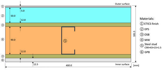
Figure 1.
Reference facade LSF wall horizontal cross-section: materials and geometry.

Table 1.
Reference facade LSF wall material thickness () and thermal conductivities ().
2.1.2. Thermal Break Strips
All the thermal break (TB) strips evaluated have a rectangular cross-section: 50 mm wide by 10 mm thick. The TB strips were placed along the inner, outer and on both sides of the metallic stud flanges, as displayed in Figure 2. They were fixed by compression between the steel studs and the OSB sheathing panels, which were attached to the steel frame using self-drilling screws. Moreover, three materials were tested in the TB strips, namely: recycled rubber and cork composite (R0), recycled rubber (R1) and aerogel (AG). These materials were chosen given their decreasing thermal conductivities, extending from 122 mW/(m∙K) down to 15 mW/(m∙K), as illustrated in Table 2.
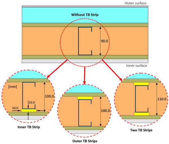
Figure 2.
Geometry and location of the thermal break (TB) strips.
Table 2.
Thermal break strips: material and thermal conductivity ().
Notice that when one or two TBS are attached to the steel stud flanges, the total thickness of the LSF wall is also increased since the steel profiles were always the same. The wall thickness increment is equal to the thickness of the TBS used, i.e., 10 or 20 mm, for one or two TBS, respectively (see Figure 2).
2.2. Experimental Lab Tests
The laboratorial tests were performed using the same experimental setup, as well as the same test procedures and set-points, used in a previous research work to evaluate the thermal performance of partition LSF walls [30]. Therefore, to avoid unnecessary repetitions and for sake of brevity, only the main issues are explained next. More detailed info about this experimental lab test can be found in Reference [30].
2.2.1. Experimental Setup
The thermal performance of the facade LSF elements were assessed making use of the heat flow meter (HFM) method [36]. However, as suggested by Rasooli and Itard [37], this method was modified, having two HF sensors. To ensure a nearly-steady-state difference of temperature, between both surfaces of the tested LSF facade sample, a set of two small climatic boxes was used: one hot (heated using an electric resistance) and another cold (cooled using an attached fridge), as displayed in Figure 3.
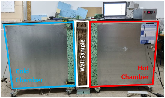
Figure 3.
Cold and hot boxes apparatus used in the experiments.
Since the moisture content of the materials, used during the experiments, can strongly conditionate their thermal properties (e.g., thermal conductivity), a stable relative humidity (RH) condition was ensured during and before the lab tests (storage stage).
Two small fans (one for each climatic chamber), reutilized from old computer case fans (12 V, 0.25 A), were used inside hot and cold boxes to promote air circulation and avoid air temperature stratification [37]. Additionally, near the wall sample (10 cm apart) a black radiation shield was placed, one inside the cold box and another one inside the hot box (not illustrated here). This radiation shield was made of PVC and it was placed at vertical position, parallel to the LSF wall test specimen.
The steel frames of the LSF wall test samples (1030 mm by 1060 mm) have three vertical steel studs, where the central one is positioned exactly in the middle, as displayed in Figure 4a. Given the high thermal conductivity of steel, to minimize the lateral heat flow, the LSF wall sample perimeter was covered by two layers (40 mm thick each) of polyurethane foam insulation, ensuring an additional edge thermal resistance of 2.22 m2·K/W.
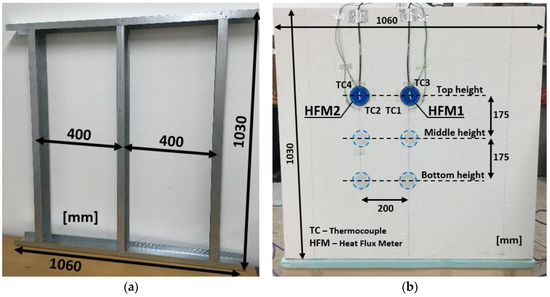
Figure 4.
Tested LSF wall sample. (a) Steel frame. (b) Sensors’ position (cold surface).
To increase the precision of the measurement and reduce its time duration (see Reference [38]), instead of the standard use of only one heat flux meter (HFM) placed in the inner side (hot) of the wall sample, another HFM was simultaneously placed in the outer side (cold). Figure 4b illustrates the sensors’ position on the cold surface of the tested LSF wall sample. As shown here, to adequately characterize the thermal resistance of the LSF wall samples, the sensors were placed in two vertical alignments: (1) near the central steel stud, where the heat flow is higher (HFM1); and (2) in the middle of the insulation cavity, where the heat flow is lower (HFM2).
In addition to heat flow, the sample surface and air temperatures were also measured, making use of certified (class one precision) type K thermocouples (TCs). To ensure the good temperature measurement accuracy of these TCs, they were previously calibrated for a temperature range [5 °C; 45 °C], with a 5 °C increment, by immersing the TCs in a thermostatic stirring water bath.
Six TCs were used in the hot side and another six in the cold side, with their locations symmetrical with regards to the hot and cold environments. Looking to the cold surface of the wall sample (Figure 4b): two TCs (TC1 and TC2) were used to measure the wall surface temperatures; another two (TC3 and TC4) were used to measure the air temperature between the wall surface and the radiation shield; and the remaining two (TC5 and TC6) measured the environment air temperature inside each chamber (not illustrated).
To record all the data obtained by the HFMs and the TCs during the experiments, one datalogger (PICO TC-08) was used on each surface of the LSF facade sample (cold and hot). Moreover, these two dataloggers were coupled to a computer (see Figure 3, over the “Hot Chamber”), where the PicoLog® version 6.1.10 software (Pico Technology Limited, St Neots, UK) was used to manage the recorded data.
To illustrate some recorded data, Figure 5 displays, for the reference LSF facade wall, the measured surface temperatures and the variation in heat flux densities over time when sensors are placed at top height location (see Figure 4b). As expected, during the first measurement hours, there is some variation in the recorded values, but after this stabilizing period there is clearly a convergence. Moreover, the temperature difference is slightly higher for the thermocouples placed in position 2 (cavity, Figure 5b) and the heat flux density is significantly smaller when compared with the sensors located at the vicinity of the steel stud (position 1, Figure 5a). Thus, the measured local thermal resistance will be much higher at this cavity location, in comparison with the steel studs’ location. This relevant thermal resistance reduction was expected, being related to the high thermal conductivity of steel and the consequent thermal bridge phenomenon occurring near this LSF wall location (position 1), even having a 50 mm continuous insulation thickness (ETICS).
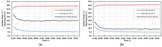
Figure 5.
Measured surface temperatures and variations in heat flux densities over time when sensors are located at top height (see Figure 4b), for the reference LSF facade wall. (a) Sensors’ position 1—stud. (b) Sensors’ position 2—cavity.
2.2.2. Set-Points and Test Procedures
To measure the surface-to-surface R-value (or thermal resistance) of the assessed LSF facade walls, using the heat flow meter (HFM) method, the test procedures prescribed in some international standards were adopted, including ISO 9869-1 [36], ASTM C 1155-95 [39] and ASTM C 1046-95 [40]. More specifically, the “summation technique” described in the standard ASTM C 1155-95 [39] was adopted, with this methodology having some similarities to the “average method” described in standard ISO 9869-1 [36]. According to the so-called “summation technique” [39], the estimated measured thermal resistance for each time interval, , could be computed making use of the following equation
where: and are the interior (hot) and exterior (cold) surface temperatures (°C), respectively; is the heat flux density (W/m2); is the counter for summation of time-series data; and is number of time values.
As suggested by this standard [39], the duration of each test was 24 h (minimum). The convergence factor and criterion are also defined in ASTM C 1155-95 [39] and given by the following expression
where: is the convergence factor; is the estimated measured thermal resistance during the evaluated time interval (e.g., 1 h); and is the estimated thermal resistance during the previously evaluated time interval. This adopted convergence criterion means that the variation in the estimated measured R-value, between a time interval and the previous one, should be smaller than 10%, in relation to the actual time interval.
As already mentioned before, the improvement suggested by Rasooli and Itard [37] was adopted to reduce test duration and increase precision, which consists of the use of two HFMs simultaneously at both cold and hot wall surfaces, as an alternative to measuring only one side, as given by ISO 9869-1 [36].
The adopted set-points for the cold and hot chambers were 5 °C and 40 °C, respectively. The measurements were performed in a quasi-steady-state heat transfer state. This large temperature difference (35 °C) between the cold and hot chambers allowed the reliability and accuracy of the measured R-values to be increased [36].
As illustrated in Figure 4b, three height sensor locations were chosen, for each wall configuration, namely: (1) top, (2) middle and (3) bottom, with one test performed for each one. Thus, the overall surface-to-surface thermal resistance of the LSF facade was achieved by averaging the values from the previously mentioned three tests, this way ensuring the repeatability of the experimental measurements.
Making use of the data recorded (heat fluxes and temperatures) for each test and applying the HFM method [36], two distinct conductive local R-values were obtained: (1) a lower value for location 1 (Figure 4), i.e., in the vicinity of the steel studs (); and (2) a higher value between the steel studs, i.e., in the middle of the insulation cavity (). The overall surface-to-surface R-value of the wall () was obtained by computing an area weighted of both measured conductive R-values, as indicated in the following equation
where: is the total area of the LSF wall (m2); is the area of influence of the steel stud (m2); and is the remaining cavity area of the LSF wall (m2).
The steel stud influence area () was defined as prescribed by ASHRAE zone method [41], i.e., assuming a zone factor () equal to 2.0 [22]. Therefore, the width of the steel stud influence zone (w) is equal to the flange length () plus two times the thickness of the thicker sheathing layer ().
Notice that these computations to obtain an overall R-value of the tested LSF wall were performed making use of a representative wall zone area defined by the studs’ spacing (width) and assuming one meter high (length), i.e., 0.40 m by 1.00 m (0.40 m2).
2.2.3. Experimental Procedures’ Verification
The verification of the reliability and good working conditions of the sensors and dataloggers, in the experimental apparatus, was performed under two different approaches: (1) testing a homogenous extruded polystyrene (XPS) panel (60 mm thick) under the same lab conditions, with known thermal conductivity and resistance; (2) simulating a representative LSF wall cross-section using some finite element models, as described in Section 2.3, and comparing the predicted R-value with the measured thermal resistance.
Regarding the first verification, both measured and manufacturer surface-to-surface thermal resistances were the same (1.784 m2∙K/W). Concerning the second verifications, as displayed later in Section 3.1 (Table 3), there was a very good agreement between the measured and the predicted R-values, the differences ranging between 0% and −3%.
Table 3.
Thermal resistances (surface-to-surface) predicted (THERM) and measured.
Moreover, Figure 6 displays the estimated measured R-values’ variation over time, at three different sensor height positions, as well as the predicted THERM R-value for the reference LSF facade wall. As expected, during the first hours of measurements, there is a convergence phenomenon until the quasi-stationary state is reached (around seven hours). After this period, the convergence criterion is reached (see Equation (2)) and the averaged measured R-values become very similar to the predicted THERM value. In fact, using the average of the measured R-values during the convergence period, the predicted and measured thermal resistances are the same (3.200 m2·K/W).
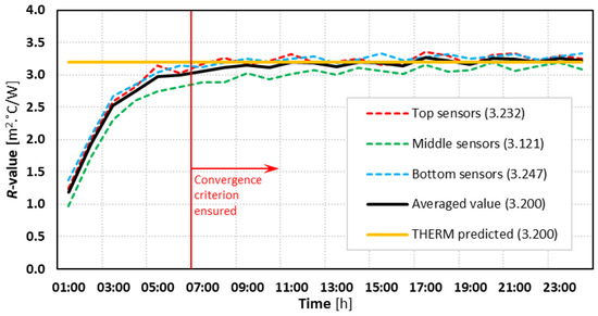
Figure 6.
Estimated measured thermal resistances’ variation over time, three different sensor heights’ locations and the predicted THERM R-value for the reference LSF facade wall.
All these verifications allowed the good working conditions of the experimental apparatus to be evidenced, to ensure the reliability of the measurements, as well as the THERM models.
2.3. Numerical Simulations
The bidimensional simulations of the LSF facades’ thermal performance were achieved using the Finite Element Method (FEM) commercial software THERM® (version 7.6.1, Lawrence Berkeley National Laboratory, United States Department of Energy: Berkeley, CA, USA). The corresponding model details are briefly explained next.
This algorithm makes use of 2D steady-state conservation of energy equation for isotropic materials
where: is the density (kg/m3); is the specific heat capacity (J/(kg·K); is the velocity (m/s); is the temperature (°C or K); λ is the thermal conductivity (W/(m·K)); and represents the volumetric heat source (W/m3).
Given the repetitive features of this LSF facade structure, as previously illustrated in Figure 1, only a typical 2D portion of the facade cross-sections (with 400 mm length) was implemented in the THERM models. The predicted R-values were computed in these models along the inner wall surface (Figure 1). In Section 2.1 (Table 1 and Table 2) the materials’ thermal properties used in the simulations were presented earlier. Additionally, for all models built in this work, a maximum error of 2% on the FEM computations was set.
For each THERM model, two sets of boundary conditions were defined, namely the air temperatures and the surface R-values. The colder external (5 °C) and warmer internal (40 °C) air temperatures were defined equal to the set-points defined for the cold and hot climatic chambers during the laboratory measurements, respectively (see Section 2.2.2). Nevertheless, as is well known, since the R-values are computed for a unitary temperature difference, they do not rely on the chosen temperature difference between interior and exterior environments.
The surface thermal resistances used in the THERM models were set equal to the average values measured for each LSF wall surface and for each test, considering the air and surface temperature differences, as well as the recorded heat fluxes in the wall surfaces. The measured surface R-values, ranging between 0.10 and 0.15 m2∙K/W, were near the value defined in ISO 6946 [42] for the internal surface resistance () when there is a horizontal heat flow, i.e., 0.13 m2∙K/W. These measured values were not even smaller because the fans used were not powerful, having reduced dimensions (only 10 by 10 cm) and oriented to the opposite side of the test-sample wall. Moreover, the black radiation shields provide some protection, uniformizing the air flux near the wall test-sample outer surface.
Several verifications were made to ensure a good accuracy of the THERM models, explicitly: (i) 2D test cases’ verification prescribed in ISO 10211 [43]; (ii) computations assuming simplified homogeneous wall layers; and (iii) validation using experimental laboratory measurements.
The two ISO 10211 [43] 2D test cases were modelled with success and the THERM software FEM algorithm for steady-state heat transfer simulations was classified as a high precision algorithm. Furthermore, the authors have a large amount of experience of using this software, as can be seen in these references [21,22,30,33].
Regarding the homogeneous wall layers’ verification, the reference LSF facade wall (illustrated in Figure 1), was modelled without the steel studs, and it was assumed the other wall layers were homogenous and continuous. Using this simplified wall model, the analytical solution could be applied since it is well known, being prescribed in ISO 6946 [42]. In this case, the total thermal resistance is calculated as the summation of the layer’s thermal resistances. Figure 7b illustrates the obtained results, where, as expected, both analytic and THERM R-values are the same when it is assumed there are homogeneous layers within the facade wall (4.283 m2∙K/W).
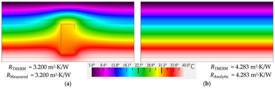
Figure 7.
Accuracy verification of the THERM models: temperature distribution and conductive R-values. (a) Inhomogeneous layers. (b) Homogeneous layers.
Concerning the lab measurements’ verification, Figure 6a also illustrates the measured overall surface-to-surface R-values of the reference facade LSF wall. The measured R-value is equal to the predicted THERM value (3.200 m2∙K/W), ensuring an excellent agreement among simulated and predicted surface-to-surface R-values, even with all the related uncertainties.
Moreover, even with a continuous exterior thermal insulation, it is very clear that, in the foreseen temperature color distribution (Figure 7), the consequence of the steel stud thermal bridge was originated by the higher heat transfer. This higher heat transfer meaningfully decreases the R-value of the facade when related with the simplified model, having homogeneous layers, i.e., without steel studs. This thermal resistance decrease was 1.083 m2∙K/W (−25%).
3. Results
The achieved results are structured here into three subsections. First, the measured and the predicted thermal resistance values are displayed. Next, the measured thermal resistance improvements due to the use of thermal break (TB) strips are graphically exhibited. Finally, the infrared thermography technic is used to better visualize the steel studs’ thermal bridges effect.
3.1. Measured and Predicted R-Values
The obtained measured and predicted results for the evaluated load-bearing LSF facade walls are displayed in Table 3, with these results being organized by the position and material of the TB strips, but starting with the reference LSF facade wall (without any TB strips). As displayed here, the agreement between the predicted and the measured R-values is very good. These differences range between −3% and 0%.
In Table 3, the thermal resistance increase that originated from using TB strips along the metallic profile flanges is well visible. This increase is bigger for materials with smaller thermal conductivities (e.g., AG—aerogel), as well as when two TB strips are used.
3.2. Measured Thermal Resistance Improvement
To better visualize these features in a graphical way, Figure 8a shows the thermal performance improvement originated by the TB strips’ use on the LSF facades, with the thermal resistance increase ranging from +4% (for the inner recycled rubber, R1in) up to +28% (for the double aerogel TB strips, AG × 2). As expected, the outer and inner TB strips’ performances are quite analogous, being a little better when placed in the outer stud flange (+1%).
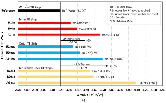
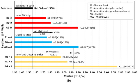
Figure 8.
Measured thermal resistances of load-bearing LSF walls. (a) Facade LSF walls. (b) Partition LSF walls (adapted from [30]).
The major R-value increase occurred when two TB strips were used (×2) and for lower thermal conductivity of the TB strip material, i.e., aerogel, AG. Indeed, the aerogel TB strips displayed a considerable increase in the obtained thermal resistances: +15% and +14% for outer and inner strips, respectively, as well as +28% when using two TB strips. However, it was not possible to reach the thermal resistance provided by a homogeneous wall without steel studs (4.283 m2∙K/W), as previously presented in Figure 7b, not even with the greatest thermal performance configuration, i.e., when having two aerogel TB strips (4.093 m2∙K/W).
To compare these facade LSF wall measurements with previous load-bearing partition LSF wall measured R-values (see Reference [30]), Figure 8b also exhibits these former values. Starting this comparison by using the reference R-values without TB strips, the facade LSF wall has a significantly higher thermal resistance (3.200 m2∙K/W) due to the use of ETICS, when compared with the partition LSF wall (1.558 m2∙K/W), corresponding to a reference R-value increase of 1.642 m2∙K/W (+105%).
Comparing now these measurement results using TB strips for the facade (Figure 8a) with the partition LSF walls (Figure 8b), both plots show a similar tendency, with the thermal resistances being higher for the facade LSF walls, as already justified and previously noticed. However, the thermal performance improvement due to the use of TB strips is now very reduced in the facade LSF walls (Figure 8a), both in absolute values (m2∙K/W) and even more evident in percentage values.
3.3. Infrared Thermography Assessment
To better visualize the differences regarding the steel studs’ thermal bridge effect between the facade and the partition LSF walls, with and without TB strips, some infrared images are displayed in Figure 9. In the partition LSF walls (Figure 9b) the presence of the middle vertical steel stud when there is no TB strip (left image) is well visible, as is the reduction in the thermal bridge effect when two aerogel TB strips are used (right image).
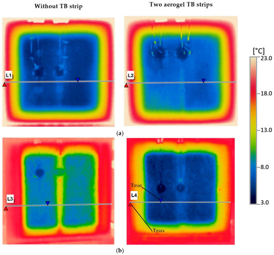
Figure 9.
IR images of the LSF walls: cold surface. (a) Facade LSF walls. (b) Partition LSF walls (adapted from [30]).
However, in the facade LSF walls (Figure 9a), the presence of the vertical central steel stud is not clearly visible, even when there are no TB strips (left image). To see this singularity in more detail, Figure 10 exhibits the surface temperatures along the horizontal lines previously displayed in Figure 9. In this plot the significant peak temperature rises near the central steel stud in the partition LSF wall are even more perceptible (Line 3), as well as the corresponding attenuation due to the use of two aerogel TB strips (Line 4). Again, in the facade wall, with a continuous thermal insulation (ETICS), this steel stud thermal bridge-related temperature increase in the middle of the LSF wall is extremely limited when there are no TB strips (Line 1), and almost negligible when there are two TB strips (Line 2).
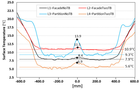
Figure 10.
Cold surface temperatures along horizontal lines obtained from thermographic images of the measured facade and partition LSF walls, with and without thermal break (TB) strips made from aerogel.
4. Discussion of Results
To provide an easier comparison of their overall performances, the charts in Figure 11 exhibit the thermal resistance improvements due to the use of TB strips, for both facade (in red color) and partition (in black color) LSF walls.
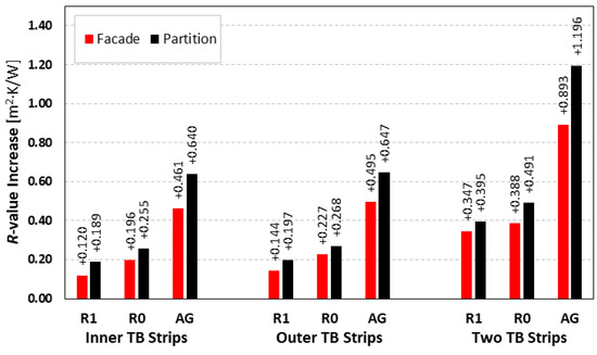
Figure 11.
The increase in thermal resistances due to thermal break (TB) strips’ use in load-bearing LSF walls: facade vs partition [30].
From the previous plots (Figure 11), it can be concluded that the TB strips are clearly less efficient in facade LSF walls when compared to partition LSF walls. This feature is related with the use of a continuous external thermal insulation layer (ETICS) in facade walls (in this case 50 mm of EPS), decreasing in this way the relevance of the thermal bridges originated by the steel studs. Additionally, the thermal resistance increases due to aerogel (AG) TB strips remain very relevant. In fact, this thermal performance improvement is about three times bigger when compared to recycled rubber (R1). Moreover, the thermal resistance rises due to the TB strips made from rubber/cork composite (R0) are only a little bigger when compared to recycled rubber (R1), i.e., about +0.08 m2·K/W for single TB strips and even lower for double TB strips (+0.04 m2·K/W).
Notice that, in all evaluated LSF walls, the use of TB strips allowed their thermal performance to be improved, by increasing the overall R-value of the wall. Obviously, with the higher thermal resistance and the lower thermal transmittance (or U-value) and, therefore, less thermal energy being lost or transferred across the wall, the energy efficiency is increased.
5. Conclusions
In this paper, a new set of experimental lab measurements was performed to evaluate the thermal performance improvement in Lightweight Steel Frame (LSF) facade walls due to the use of thermal break (TB) strips. Three different materials were evaluated as TB strips, namely: recycled rubber (R1); recycled rubber/cork composite (R0); and aerogel (AG), for three different TB strip positions along the steel stud flanges: inner, outer and on both sides (double).
Notice that all the measured R-values were related with the simulation results achieved using implemented numerical bidimensional finite element models. These comparisons provided excellent thermal resistance agreements, within an error range of ±3%, for the ten evaluated facade LSF walls, ensuring good reliability, as well as a high robustness of the test procedures and implemented measurement apparatus.
This research work has provided new developments of a previous study regarding the experimental assessment of TB strips’ performance in non-load-bearing and load-bearing LSF walls [30]. In this case, instead of partition walls, load-bearing facade LSF walls were evaluated, usually with a continuous external thermal insulation composite system (ETICS).
Taking the previous study for load-bearing partition LSF walls as a reference also [30], the main conclusions are summarized as follows:
- The outer and inner TB strips still have very similar thermal performances. However, as happened before for partition walls, the TB strips positioned in the outer steel flange of the facade LSF walls appear to have slightly better performance (around +1% in the measured R-value).
- Again, as expected, the best performances were found for double TB strips and for aerogel TB strips.
- However, neither the former load-bearing partition LSF wall, neither this new facade LSF wall, were able to fully mitigate the steel frame thermal bridges’ effect, not even for the best thermal performance configuration (two aerogel TB strips).
- Quite similar thermal performances were measured for the other two materials: recycled rubber (R1), and rubber/cork composite (R0).
- Comparing the thermal resistance improvement for these facade LSF walls and the previously assessed partition LSF walls, it was observed that the TB strips were clearly less efficient in facade LSF walls.
This last conclusion can be justified by the existence of a continuous external thermal insulation layer (ETICS) in the facade walls (in this case 50 mm of EPS), decreasing the relevance of the thermal bridges originated by the steel studs. Consequently, the efficiency of the TB strips becomes reduced.
Notice that the improved thermal resistances due to the use of TBS were caused not only to the TB strips themselves, but also provided by the increased total thickness of the LSF wall, particularly the increased thickness of the expansible mineral wool thermal insulation, placed inside the wall cavity.
This research allowed the effectiveness of TB strips for the R-values’ increase in partition and facade load-bearing LSF walls to be better comprehended, quantified and compared, information that was not available in the literature, particularly for facade LSF walls. Additionally, the measured conductive thermal resistances can be used, for the validation of numerical simulations in LSF walls with identical arrangements, as benchmark values.
Author Contributions
Conceptualization, P.S. and D.M.; Formal analysis, P.S., D.M., D.F. and A.V.; Funding acquisition, P.S.; Investigation, P.S., D.M., D.F. and A.V.; Methodology, P.S. and D.M.; Project administration, P.S.; Resources, P.S.; Supervision, P.S.; Validation, P.S.; Writing—original draft, P.S.; Writing—review & editing, P.S., D.M., D.F. and A.V. All authors have read and agreed to the published version of the manuscript.
Funding
This research was funded by FEDER funds through the Competitivity Factors Operational Programme, COMPETE, and by national funds through FCT, Foundation for Science and Technology, within the scope of the project POCI-01-0145-FEDER-032061.
Acknowledgments
The authors also want to thank the support provided by the following companies: Pertecno, Gyptec Ibéria, Volcalis, Sotinco, Kronospan, Hulkseflux, Hilti and Metabo.
Conflicts of Interest
The authors declare no conflict of interest.
References
- Farouk, N.; El-Rahman, M.A.; Sharifpur, M.; Guo, W. Assessment of CO2 emissions associated with HVAC system in buildings equipped with phase change materials. J. Build. Eng. 2022, 51, 104236. [Google Scholar] [CrossRef]
- European Union. Directive (EU) 2018/844 of the European Parliament and of the Council of 30 May 2018 amending Directive 2010/31/EU on the energy performance of buildings and Directive 2012/27/EU on energy efficiency. Off. J. Eur. Union 2018, 2018, 75–91. [Google Scholar]
- D’Agostino, D.; Tzeiranaki, S.T.; Zangheri, P.; Bertoldi, P. Assessing Nearly Zero Energy Buildings (NZEBs) development in Europe. Energy Strateg. Rev. 2021, 36, 100680. [Google Scholar] [CrossRef]
- Bustos García, A. Morteros con Propiedades Mejoradas de Ductilidad por Adición de Fibras de Vidrio, Carbono y Basalto. Doctoral Thesis, Universidad Politécnica de Madrid, Madrid, Spain, 2018. (In Spanish). [Google Scholar]
- European Commission. The European Green Deal. In Communication from the European Comission: COM/2019/640 Final, 11.12.2019; EUR-Lex: Brussels, Belgium, 2019. [Google Scholar]
- Cutanda, B.L.; Turrillas, J.C.A. Administración y Legislación Ambiental, 11th ed.; Dykinson: Madrid, Spain, 2020; ISBN 978-84-1324-302-3. [Google Scholar]
- Buckley, N.; Mills, G.; Reinhart, C.; Berzolla, Z.M. Using urban building energy modelling (UBEM) to support the new European Union’s Green Deal: Case study of Dublin Ireland. Energy Build. 2021, 247, 111115. [Google Scholar] [CrossRef]
- Rezai, S.H.; Allard, F.; Abelé, C.; Doya, M. Evaluating External Thermal Insulation Composite Systems (ETICS) regarding the building’s global performance. Energy Procedia 2015, 78, 1562–1567. [Google Scholar] [CrossRef]
- Parracha, J.; Borsoi, G.; Flores-Colen, I.; Veiga, R.; Nunes, L.; Dionísio, A.; Gomes, M.G.; Faria, P. Performance parameters of ETICS: Correlating water resistance, bio-susceptibility and surface properties. Constr. Build. Mater. 2021, 272, 121956. [Google Scholar] [CrossRef]
- Fernandes, C.; de Brito, J.; Cruz, C.O. Architectural integration of ETICS in building rehabilitation. J. Build. Eng. 2016, 5, 178–184. [Google Scholar] [CrossRef]
- Luján, S.V.; Arrebola, C.V.; Sánchez, A.R.; Benito, P.A.; Cortina, M.G. Experimental comparative study of the thermal performance of the façade of a building refurbished using ETICS, and quantification of improvements. Sustain. Cities Soc. 2019, 51, 101713. [Google Scholar] [CrossRef]
- Kolaitis, D.I.; Malliotakis, E.; Kontogeorgos, D.A.; Mandilaras, I.; Katsourinis, D.I.; Founti, M.A. Comparative assessment of internal and external thermal insulation systems for energy efficient retrofitting of residential buildings. Energy Build. 2013, 64, 123–131. [Google Scholar] [CrossRef]
- Santos, P.; da Silva, L.S.; Ungureanu, V. Energy Efficiency of Light-Weight Steel-Framed Buildings, 1st ed.; Technical Committee 14—Sustainability & Eco-Efficiency of Steel Construction; European Convention for Constructional Steelwork (ECCS): Brussels, Belgium, 2012; ISBN 978-92-9147-105-8. [Google Scholar]
- Choi, J.-S.; Kim, C.-M.; Jang, H.-I.; Kim, E.-J. Detailed and fast calculation of wall surface temperatures near thermal bridge area. Case Stud. Therm. Eng. 2021, 25, 100936. [Google Scholar] [CrossRef]
- Liu, C.; Mao, X.; He, L.; Chen, X.; Yang, Y.; Yuan, J. A new demountable light-gauge steel framed wall: Flexural behavior, thermal performance and life cycle assessment. J. Build. Eng. 2022, 47, 103856. [Google Scholar] [CrossRef]
- Perera, D.; Poologanathan, K.; Gillie, M.; Gatheeshgar, P.; Sherlock, P.; Upasiri, I.; Rajanayagam, H. Novel conventional and modular LSF wall panels with improved fire performance. J. Build. Eng. 2022, 46, 103612. [Google Scholar] [CrossRef]
- Alembagheri, M.; Sharafi, P.; Rashidi, M.; Bigdeli, A.; Farajian, M. Natural dynamic characteristics of volumetric steel modules with gypsum sheathed LSF walls: Experimental study. Structures 2021, 33, 272–282. [Google Scholar] [CrossRef]
- Tavares, V.; Soares, N.; Raposo, N.; Marques, P.; Freire, F. Prefabricated versus conventional construction: Comparing life-cycle impacts of alternative structural materials. J. Build. Eng. 2021, 41, 102705. [Google Scholar] [CrossRef]
- Perera, D.; Upasiri, I.; Poologanathan, K.; Gatheeshgar, P.; Sherlock, P.; Hewavitharana, T.; Suntharalingam, T. Energy performance of fire rated LSF walls under UK climate conditions. J. Build. Eng. 2021, 44, 103293. [Google Scholar] [CrossRef]
- Moga, L.; Petran, I.; Santos, P.; Ungureanu, V. Thermo-Energy Performance of Lightweight Steel Framed Constructions: A Case Study. Buildings 2022, 12, 321. [Google Scholar] [CrossRef]
- Santos, P.; Gonçalves, M.; Martins, C.; Soares, N.; Costa, J.J. Thermal Transmittance of Lightweight Steel Framed Walls: Experimental versus Numerical and Analytical Approaches. J. Build. Eng. 2019, 25, 100776. [Google Scholar] [CrossRef]
- Santos, P.; Lemes, G.; Mateus, D. Analytical Methods to Estimate the Thermal Transmittance of LSF Walls: Calculation Procedures Review and Accuracy Comparison. Energies 2020, 13, 840. [Google Scholar] [CrossRef]
- Santos, P.; Poologanathan, K. The Importance of Stud Flanges Size and Shape on the Thermal Performance of Lightweight Steel Framed Walls. Sustainability 2021, 13, 3970. [Google Scholar] [CrossRef]
- Roque, E.; Santos, P. The Effectiveness of Thermal Insulation in Lightweight Steel-Framed Walls with Respect to Its Position. Buildings 2017, 7, 13. [Google Scholar] [CrossRef]
- Roque, E.; Santos, P.; Pereira, A.C. Thermal and sound insulation of lightweight steel-framed façade walls. Sci. Technol. Built Environ. 2019, 25, 156–176. [Google Scholar] [CrossRef]
- Santos, P.; Ribeiro, T. Thermal Performance of Double-Pane Lightweight Steel Framed Walls with and without a Reflective Foil. Buildings 2021, 11, 301. [Google Scholar] [CrossRef]
- Santos, P.; Ribeiro, T. Thermal Performance Improvement of Double-Pane Lightweight Steel Framed Walls Using Thermal Break Strips and Reflective Foils. Energies 2021, 14, 6927. [Google Scholar] [CrossRef]
- Santos, P.; Abrantes, D.; Lopes, P.; Mateus, D. Experimental and Numerical Performance Evaluation of Bio-Based and Recycled Thermal Break Strips in LSF Partition Walls. Buildings 2022, 12, 1237. [Google Scholar] [CrossRef]
- Martins, C.; Santos, P.; da Silva, L.S. Lightweight steel-framed thermal bridges mitigation strategies: A parametric study. J. Build. Phys. 2016, 39, 342–372. [Google Scholar] [CrossRef]
- Santos, P.; Mateus, D. Experimental assessment of thermal break strips performance in load-bearing and non-load-bearing LSF walls. J. Build. Eng. 2020, 32, 101693. [Google Scholar] [CrossRef]
- WEBERTHERM UNO. Technical Sheet: Weber Saint-Gobain ETICS Finish Mortar. 2018. Available online: www.pt.weber/files/pt/2019-04/FichaTecnica_weberthermuno.pdf (accessed on 14 March 2019). (In Portuguese).
- TincoTerm. Technical Sheet: EPS 100. 2015. Available online: http://www.lnec.pt/fotos/editor2/tincoterm-eps-sistema-co-1.pdf (accessed on 14 March 2021). (In Portuguese).
- Santos, P.; Lemes, G.; Mateus, D. Thermal Transmittance of Internal Partition and External Facade LSF Walls: A Parametric Study. Energies 2019, 12, 2671. [Google Scholar] [CrossRef]
- Santos, C.; Matias, L. ITE50—Coeficientes de Transmissão Térmica de Elementos da Envolvente dos Edifícios; LNEC—Laboratório Nacional de Engenharia Civil: Lisbon, Portugal, 2006. (In Portuguese) [Google Scholar]
- MS-R0 Test Report. Test Report Ref. 5015 PE 1977/08—Determination of Thermal Conductivity (Acousticork MS-R0); Departamento de Engenharia Têxtil, Universidade do Minho: Braga, Portugal, 2008.
- ISO 9869-1; Thermal Insulation—Building Elements—In-Situ Measurement of Thermal Resistance and Thermal Transmittance. Part 1: Heat Flow Meter Method. ISO—International Organization for Standardization: Geneva, Switzerland, 2014.
- Soares, N.; Martins, C.; Gonçalves, M.; Santos, P.; da Silva, L.S.; Costa, J.J. Laboratory and in-situ non-destructive methods to evaluate the thermal transmittance and behaviour of walls, windows, and construction elements with innovative materials: A review. Energy Build. 2019, 182, 88–110. [Google Scholar] [CrossRef]
- Rasooli, A.; Itard, L. In-situ characterization of walls’ thermal resistance: An extension to the ISO 9869 standard method. Energy Build. 2018, 179, 374–383. [Google Scholar] [CrossRef]
- ASTM-C1155–95 (Reapproved-2013); Standard Practice for Determining Thermal Resistance of Building Envelope Components from the In-Situ Data. ASTM—American Society for Testing and Materials: Philadelphia, PA, USA, 2013.
- ASTM-C1046–95 (Reapproved-2013); Standard Practice for In-Situ Measurement of Heat Flux and Temperature on Building Envelope Components. ASTM—American Society for Testing and Materials: Philadelphia, PA, USA, 2013.
- ASHRAE. Handbook of Fundamentals (SI Edition); ASHRAE—American Society of Heating, Refrigerating and Air-conditioning Engineers: Atlanta, GA, USA, 2017. [Google Scholar]
- ISO 6946; Building Components and Building Elements—Thermal Resistance and Thermal Transmittance—Calculation Methods. International Organization for Standardization: Geneva, Switzerland, 2017.
- ISO 10211; Thermal Bridges in Building Construction—Heat Flows and Surface Temperatures—Detailed Calculations. ISO—International Organization for Standardization: Geneva, Switzerland, 2017.


Publisher’s Note: MDPI stays neutral with regard to jurisdictional claims in published maps and institutional affiliations. |
© 2022 by the authors. Licensee MDPI, Basel, Switzerland. This article is an open access article distributed under the terms and conditions of the Creative Commons Attribution (CC BY) license (https://creativecommons.org/licenses/by/4.0/).