Article

Numerical Simulation of Roughness Effects of Ice Accretion on Wind Turbine Airfoils

1
ForWind-Centre for Wind Energy Research, Institute of Physics, University of Oldenburg, 26129 Oldenburg, Germany
2
Fraunhofer Institute for Wind Energy Systems, Küpkersweg 70, 26129 Oldenburg, Germany
3
Senvion GmbH, Überseering 10, 22297 Hamburg, Germany
*
Author to whom correspondence should be addressed.
Current address: Institute of Energy and Climate Research (IEK-14), Forschungszentrum Juelich GmbH, 52425 Juelich, Germany.
Current address: Nordex Energy SE & Co., KG, Service Product Management, Langenhorner Chaussee 600, 22419 Hamburg, Germany.
Energies 2022, 15(21), 8145; https://doi.org/10.3390/en15218145
Submission received: 15 June 2022 / Revised: 24 July 2022 / Accepted: 28 August 2022 / Published: 1 November 2022
(This article belongs to the Special Issue Advanced Technologies in Wind Power Generation)

Abstract

:
One of the emerging problems in modern computational fluid dynamics is the simulation of flow over rough surfaces. A good example of these rough surfaces is wind turbine blades with ice formation on its leading edge. Instead of resolving the airflow field using a fine computational grid near the wall, rough wall functions (RWFs) can be used to model the flow behavior in case of the presence of roughness. This work aims to investigate the performance of state-of-the-art RWFs to show which of these models can provide the most accurate results with the lowest computational cost possible. This aim is achieved by comparing coefficients of lift and pressure resulting from CFD simulations with wind tunnel results of an airfoil with actual ice profiles collected from the site. The RWFs are used to simulate airflow field over the airfoil profiles with ice profile attached to its leading edge using OpenFOAM CFD framework. The comparison of the numerical simulations and the wind tunnel measurements showed that the Colebrook RWF provided the best agreement between simulation and experimental results while using about 20% of the number of cells used with smooth RWF.

1. Introduction

For the last few decades, energy generation from wind has increased rapidly as a renewable source of energy. Because of this rapidly increasing demand for wind energy, wind turbine manufacturers have been trying to increase the size of the turbine rotors. By increasing rotor diameter and tower height, the single turbine can now harvest more power from wind in almost the same horizontal area occupied by old, small size wind turbines. However, some of the best wind energy sites such as in Europe and North America suffer from icing atmospheric conditions. These conditions can decrease the annual energy production by up to 40% as shown by Sailor et al. [1]. This drop in blade aerodynamic performance occurs due to several detachments and reattachment areas on the surface due to the presence of a rough ice surface.
Since the 1930s, different experiments were conducted to understand the effect of roughness on fluid flow in general. One of the pioneers in this field was Nikuradse [2] who investigated turbulent flow in pipes with different relative roughness values and Reynolds numbers between 10 4 to 10 6 . He noticed that the boundary layer follows the log law as in the case of a smooth surface. However, in the case of rough surfaces, there is a clear velocity shift ( Δ u ) . A few years later, Schlichting [3] studied the internal flow of a square-section channel with one rough wall. This rough wall had spherical segments, cones, and angular shapes. He found that the velocity shift depends on four different geometrical parameters of roughness elements, namely: the element’s height, the area projected on the surface, the area projected in the flow direction, and the average distance between elements. Accordingly, he derived an equation to calculate the friction coefficient on the plate surface. Later, Moody [4] provided an engineering method to calculate friction losses in pipes due to roughness.
For external flow applications, Blanchard [5] and Hosni [6] provided measurements of the heat transfer performance of a heated flat plate with hemispherical roughness elements. In addition, Hosni [7] studied the effect of roughness shape on the boundary layer. Achenbach [8] studied heat transfer of a roughened circular cylinder at different roughness heights and Reynolds numbers.
From the computational point of view, it is known that to correctly model the viscous sub-layer in computational fluid dynamics (CFD) methods, the height of the grid’s first cell should fulfill the y + 1 criteria. Additionally, to avoid high aspect ratio cells, a large number of cells over the surface should be generated. Accordingly, one method to simulate rough surfaces is to generate a fine grid that fits the rough surface. Wang and Zhu [9] simulated ice accretion on the NREL Phase VI wind turbine blade. In their numerical setup, they used a grid y + 1 , which resulted in a grid with a total of 7.3 million cells for a half-cylindrical domain for one blade. This provides a good idea about how much computational cost is needed to perform such simulations in the standard way. However, this cost can be much more increased for larger turbine blades manufactured nowadays.
Another approach is to modify the mathematical models in a way that the behavior of flow over rough surfaces is grasped without the need for a fine grid. The growing use of CFD in fluid flow simulations in both research and industrial applications has caused an increased interest in this approach and more new models have been developed. The challenge is to find the proper mathematical models which are often based on the results of the aforementioned experiments. Chen and Patel [10] introduced a two-layer model and a wall function in the k- ϵ model to simulate rough surfaces. Hellsten and Laine [11] provided an extension for the k- ω SST turbulence model to simulate the behavior of flow, and so did Wilcox et al. [12] with the k- ω model. Instead of providing changes to turbulence models, rough wall functions (RWFs) were developed to simulate the behavior of turbulent flow near walls. In general, wall functions must provide adequate handling for flow change from its stream velocity to stagnation on the wall according to the no-slip condition. Thus RWFs should provide additional models that account for roughness. Recently, Da Silva et al. [13] applied a new ν t wall function base on the work of Suga et al. [14]. In addition, Knopp et al. [15] and Chedevergne and Aupoix [16] provided k and ω wall functions that are capable to adapt for the presence of roughness on the surface.
The current work aims to find a computational model that can simulate the airflow around an iced wind turbine airfoil. This model should provide the most accurate results using the least computational resources possible. This aim is approached by comparing the CFD simulation results of different RWFs with experimental results of actual wind turbine ice accretion profiles. The studied ice profiles were collected from the site and tested in a wind tunnel after being molded and attached to the airfoil. In this work, three different RWFs were implemented in OpenFOAM® v6 [17] and compared: Knopp et al. [15] RWF, which will be referred to in this work as DLR-RWF, Da Silva et al. [13] RWF, which will be referred to as Momentum-RWF, and Chedevergne and Aupoix [16] RWF fitted to Colebrook’s experimental results, which will be referred as Colebrook-RWF.
This article is structured as follows: In Section 2, the mathematical model of each of the used RWFs is shown. In Section 3, the preparation of the rough ice numerical model for the simulation and the corresponding computational mesh generation is explained. Meanwhile, in Section 4, the experimental results, the validation cases, and the results of each case studied in this work are explained. In the last section, a discussion and conclusions of this work and how these results can be applied to general rough surface simulations are provided.

2. Mathematical Models

In this section, a brief description of the RANS models used in flow field simulations is introduced as a background for the studied RWFs. Subsequently, the details of the implemented RWFs are also given.
In RANS models, Navier–Stokes equations are solved as time-averaged while an extra one equation is solved (like in Spalart–Allmaras) or two equations (like in k- ω SST) or more equations are solved to close the system of equations required to solve the flow field [18].

2.1. RANS Turbulence Models

In this work, only steady-state RANS turbulence models, namely Spalart–Allmaras [19] and Menter’s k- ω SST [20], were used to simulate the turbulent flow field over the iced airfoils. In general aerodynamic simulation problems, both models show good results, especially in the pre-stall AoA’s. However, each model has its advantages. Since Spalart–Allmaras (SA) turbulence model is a one-equation model, it is usually more stable and requires less computational power. On the other hand, k- ω SST can reach better results due to solving more turbulence parameters, but of course with more computational cost.
In this work, these two different turbulence models were specifically chosen to fit different wall functions. As will be explained in the next section, one of the used RWFs defines a relationship for turbulent kinematic viscosity ν t . This type will be used only with the SA model since it mainly solves the ν t equation to simulate the flow field. The other two RWFs adapt k and ω values near the wall for the presence of roughness. Accordingly, these two RWFs will be used only with the k- ω SST turbulence model.

2.2. Rough Wall Functions

Nikuradse [2] found that the boundary layer log-law behavior in flow over both rough and smooth surfaces is the same except for a velocity shift ( Δ u ) . The difference between most of the proposed RWFs in various literature is how to calculate this shift. Schlichting [3] worked out the parameters on which the velocity shift depends on, the four parameters: average elements height ( K a v g ), the area projected on the surface ( A p ), area projected in the flow direction ( A s ), and the average distance between elements ( L a v g ) (as shown in Figure 1) are contracted together to one dimensionless parameter called equivalent sand roughness height ( K s ) that can be calculated by the equations presented in Dirling [21]
K s K a v g = 0.0164 × Λ 3.78 for Λ < 4.93 139.0 × Λ 1.90 for Λ > 4.93
where
Λ = L a v g K a v g A p A s 4 / 3
So, once the roughness profile is known, K a v g , L a v g , and D a v g can be calculated. Assuming roughness elements take certain geometrical shape for approximation, A p and A s can be calculated.In the current study, roughness elemnts are assumed to take conical shapes. Accordingly, A p / A s = π D a v g / 2 K a v g and Equations (1) and (2) can be implemented to calculate K s . The final value of the velocity shift in all RWFs used in this work depends on the calculated value of K s .

2.2.1. Momentum RWF

Da Silva et al. [13] applied the velocity shift to the well-known log-low equation by introducing a new term, namely Δ B , that represents this velocity shift as a function of K s according to Cebeci [22] ideas in the equations
u + = 1 κ ln ( E y + Δ B )
Δ B = 0 : K s + 2.5 1 κ l n K s + 2.25 87.75 + C s K s + sin 0.4258 ( ln K s + 0.811 ) : 2.5 < K s + < 90 1 κ l n ( 1 + C s K s + ) : K s + 90
where y + = y ( 1 ) u τ / ν , K s + = u τ K s / ν , E = 9.8 , κ = 0.41 and
C s = E 32.6 1 K s +
Finally, turbulent viscosity can be calculated by:
ν t | w = ν ( y + κ ln ( E y + / e κ Δ B ) ) .
Since this wall RWF deals mainly with ν t , it is used with the Spalart–Allmaras turbulence model to simulate rough surface.

2.2.2. DLR RWF

In their work, Knopp et al. [15] followed the ideas of Aupoix and Spalart [23] in adding the velocity shift effect to the wall function. However, instead of applying the shift on turbulent viscosity as in Aupoix and Spalart [23], they used their procedure to adapt k and ω turbulence parameters. The new k and ω RWF states that
ω | w = m i n ( u τ β k 1 / 2 κ d ˜ o , 60 ν β ω y ( 1 ) 2 )
d ˜ o = 0.033 ϕ r 2 k s
ϕ r 2 = m i n ( 1 , k s + 2 / 3 30 ) m i n ( 1 , k s + 1 / 4 45 ) m i n ( 1 , k s + 1 / 4 60 )
k | w = ϕ r 2 k r o u g h
k r o u g h = u τ β k 0.5 , ϕ r 2 = m i n ( 1 , k s + 90 )
where β k = 0.09 , κ = 0.41 , β w = 0.075 . Unlike Momentum RWF explained in Section 2.2.1, this RWF deals with modifying k and ω values near the wall. Hence, this RWF is used with k- ω SST turbulence model.

2.2.3. Colebrook RWF

Chedevergne and Aupoix [16] applied Suga et al. [14] approach in adapting k and ω turbulence parameters to rough surfaces and fitted the resulting formula to Colebrook’s experimental data. This resulted in:
k | w = m a x 0 , 1 β * tanh ln k s + 90 ln 10 + 1 t a n h k s + 125 t a n h k s + 125
ω | w = 300 k s + t a n h 15 4 k s + 1 + 191 k s + 1 e x p k s + 250
Also, the same as DLR RWF, this one is used with the k- ω SST turbulence model.

3. Profiles and Grids of CFD Simulations

To enable the usage of the aforementioned RWF’s, rough ice profiles have to be smoothened to give an equivalent smooth surface. By using this smooth surface and the K s value calculated from Equation (1), the RWF’s can be used in the simulation cases. This section explains how these profiles should be prepared and how the computational grid should be generated.

3.1. Wind Turbine Airfoil with Ice Accretion

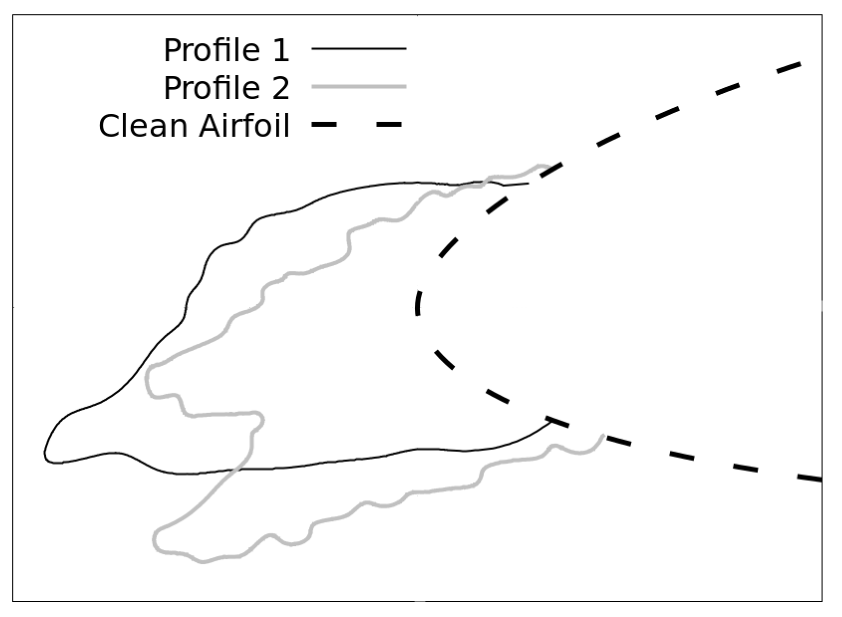
To show the different wall functions described in Section 2, they were applied on a wind turbine airfoil with two different ice accretion profiles. Both ice profiles take the horn-ice form Figure 2 which usually occur under severe icing conditions and also both of them extend to 7.5–10% of chord length. However, it can be noticed that profile 1 is smoother than profile 2. In addition, it can be noticed that profile 1 takes a more aerodynamic shape than profile 2 since profile 2 has two horns which form a stagnation area between them.

3.2. Roughness Parameters Calculations

Since all RWFs treat the rough wall as a smooth wall with a velocity shift as explained in Section 2.2, the actual rough surface of the ice profile is replaced with another equivalent smooth surface. The new smooth surface will be used to generate the computational grid around the profile and will be numerically treated as a rough surface, i.e., a velocity shift will be added to the smoothed surface. To calculate this new surface, the rough surface was smoothed with cubic splines. Similar to the calculation procedures of roughness parameters indicated in the DIN-EN-ISO 4287 standard [24], the rough surface should be smoothed as shown in Figure 3a, using a cubic spline in this work, to find an average, smooth surface. The next step is to map this smooth surface to the x-axis as shown in Figure 3b to be able to analyze the roughness parameters.
Knowing the distance between roughness elements and height of elements, the average sand roughness height explained in Figure 1 can be calculated using Equation (1). By analyzing the laser-scanned ice surfaces in different works in the literature such as Hawkins et al. [25] and McClain et al. [26], it can be assumed that roughness elements take conical shapes. Accordingly, A p = π D a v g 2 / 4 and A s = 0.5 K a v g D a v g . The above analysis provides results in K s = 1 × 10 3 m and 1 × 10 2 m for profiles 1 and 2, respectively.

3.3. Grid Generation

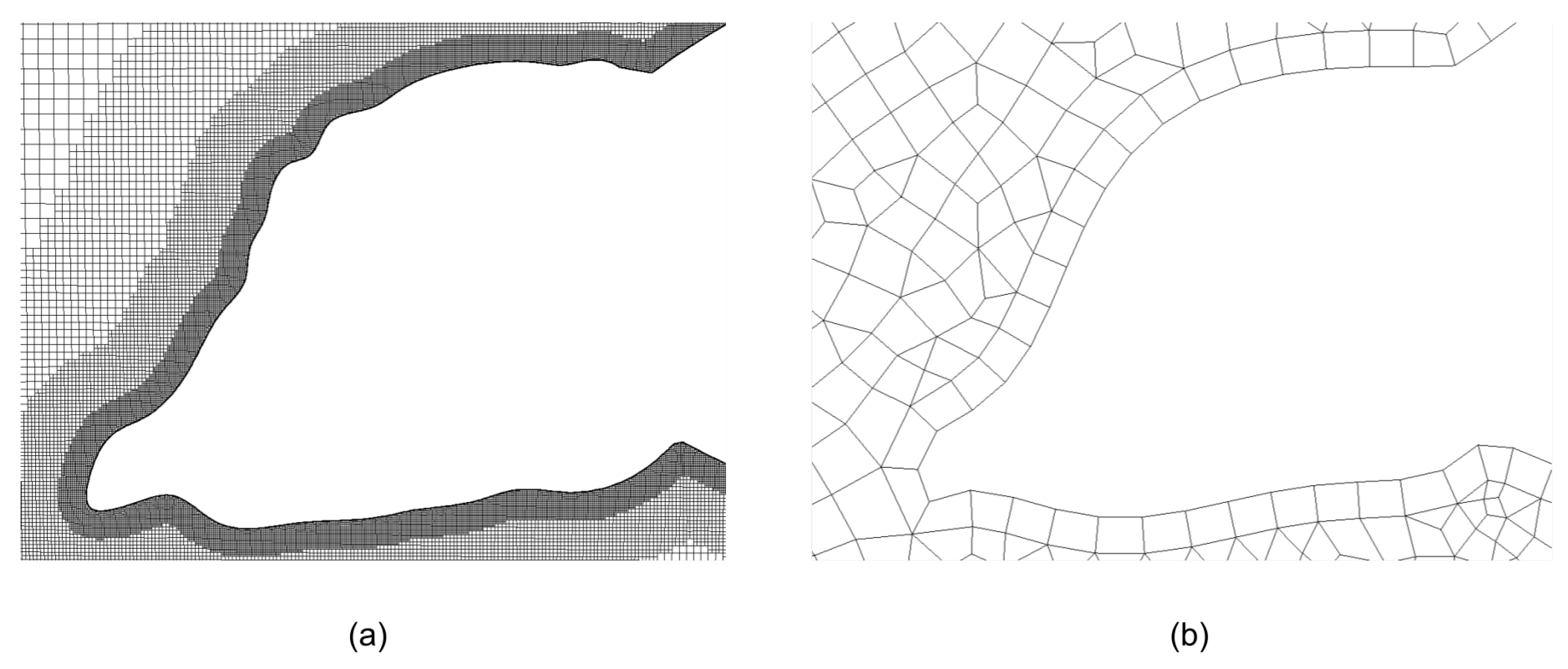
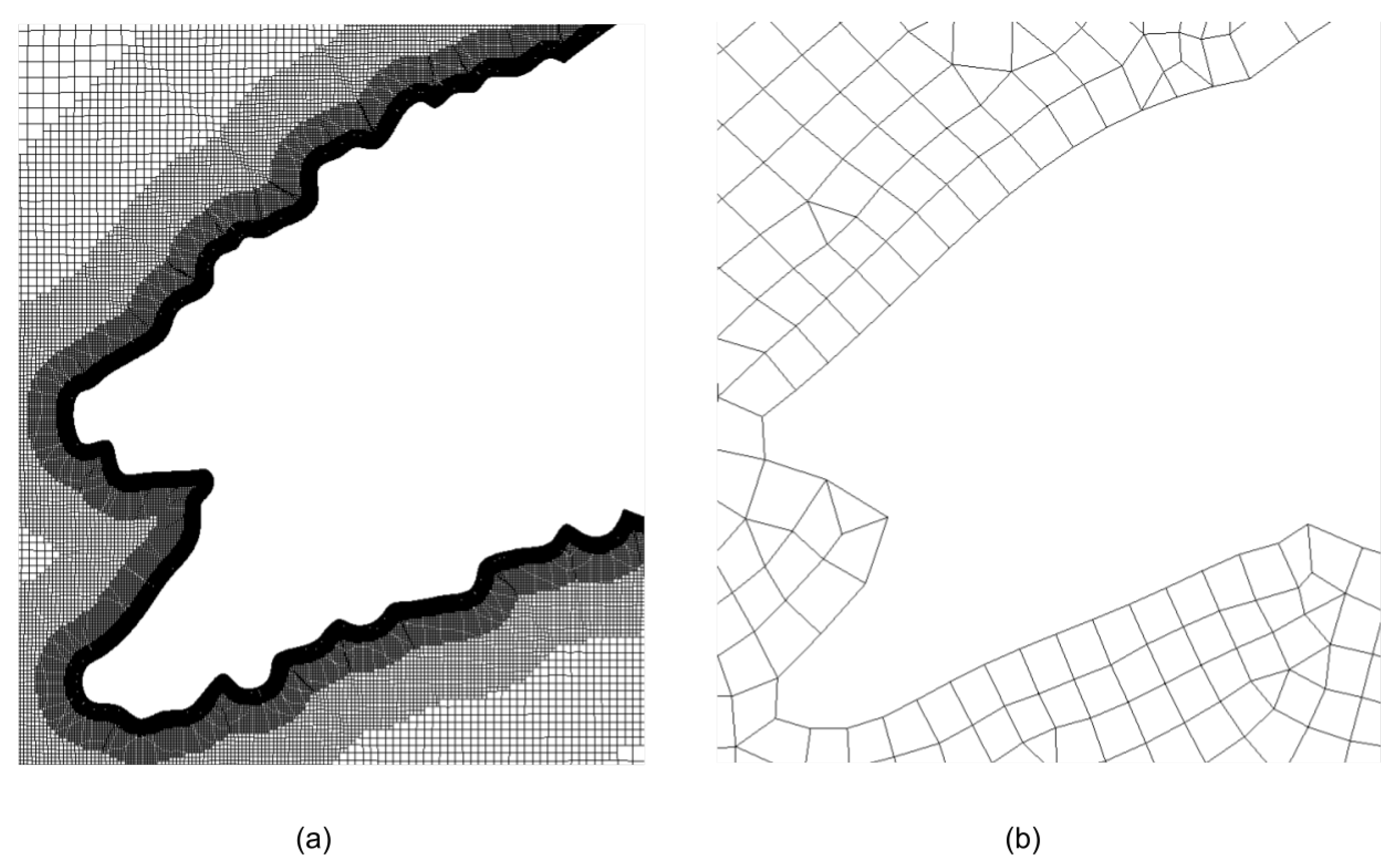
In order to use rough wall functions, the height of the first cell center should be large enough to cover the roughness element. Along with converting the rough surface into a smoother one, the resulting grid is much coarser than the grid required by smooth wall functions which require y + ( 1 ) < 1 to be able to correctly simulate the boundary layer. Accordingly, the studied approach in this work requires fewer computational resources. In the case of the two ice profiles studied in this work, properly generating a grid that fulfills the condition of y + ( 1 ) < 1 , is found to require the number of cells ≈ 4 × 10 5 cells in 2D simulations. On the other hand, when using rough wall functions with the proper first cell height and roughness smoothing, it is found to require less than 8 × 10 4 cells in 2D simulations. This means that number of cells required for the simulations using RWFs is less than 20% of the number of cells required in case of a fully resolved boundary layer. This is reflected in the computational cost to perform such simulations. A comparison between smooth and rough wall function grids is shown in Figure 4 and Figure 5. Resulting of the numerical setup described above, the properties of computational grids used in this work are given in Table 1.
To provide a comparison between the results of fully resolved surface roughness and using RWFs, the next section will also provide a comparison between C l values resulting from using fine and coarse grids, shown in Figure 5a and Figure 6a, respectively, and coarse grids, shown in Figure 5b and Figure 6b, used with RWFs.
It should be noticed that the first cell height in the case of RWF simulations is relatively larger than in the case of fully resolved mesh to fit the criteria explained by Liu [27]. This criteria mandates that the height of the cell center of the first cell near the wall should be larger than the roughness height. Accordingly, a grid independence test was conducted to select the first cell height values indicated in Table 1. The first cell heights are shown in Table 1. In these grid tests, grids with first cell heights between 4–10 mm were used to simulate the airflow around the rough ice surface after smoothing. The results of these grid tests are shown in Appendix A. Figure A1 shows the C l resulting from the used RWFs in this work for profile 1 while Figure A2 shows the C l results for profile 2.

4. Numerical Simulation Results

For simulation results, a validation case will be introduced to give evidence of the correct implementation of the new codes. Then, the results of the CFD simulation cases of airfoils with ice accretion profiles indicated in Table 1 are shown, analyzed, and evaluated.

4.1. Implementation and Validation

To apply the aforementioned RWF, Equations (7)–(13) were implemented within OpenFOAM framework. The Momentum RWF is already available in OpenFOAM (named nutURoughWallFunction). However, the other two wall functions, namely DLR and Colebrook RWF, are not available. These two wall functions were implemented and validated against experimental results published by Achenbach [8]. In this paper, the author analyzed the flow field around a circular copper cylinder with pyramidal roughness elements to study both fluid flow and heat transfer. This experiment was conducted on a 0.5 m length, 0.15 m diameter copper cylinder at different roughness heights and Reynolds numbers.
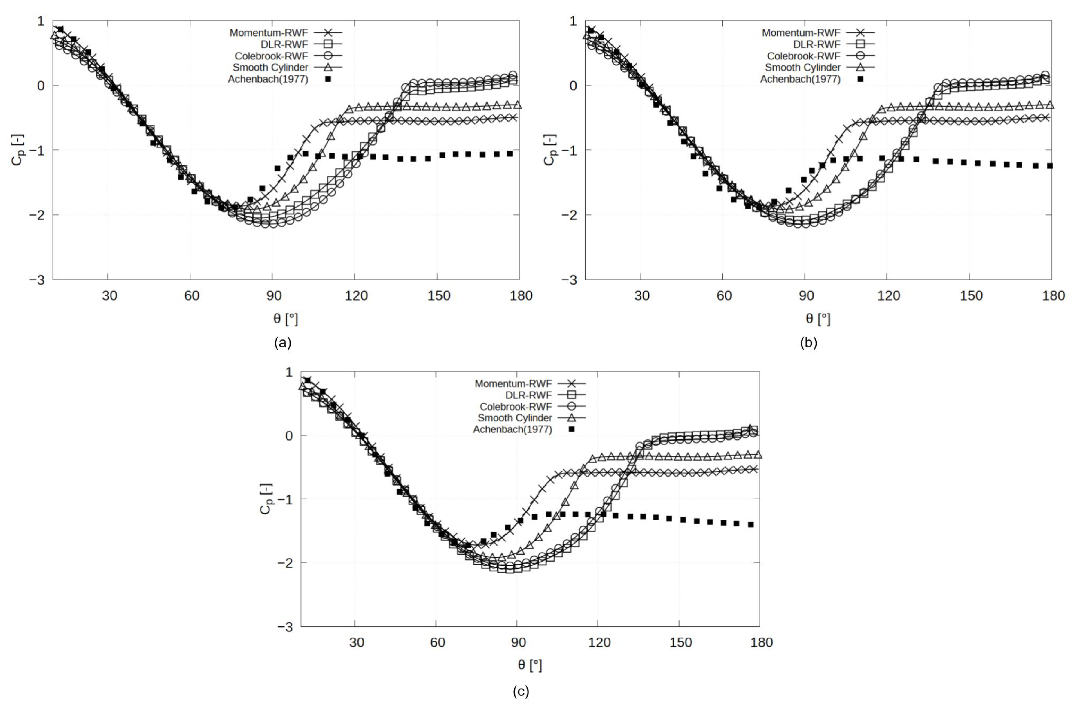
It is known that RANS simulations of the flow field around a cylinder are already unstable and hard to predict, especially when it comes to the prediction of separation location. However, this case was selected to identify any false implementation of RWFs in OpenFOAM that may lead to unstable numerical solutions. Figure 7a–c shows the results of simulating circular cylinder at R e = 4 × 10 6 and K s = 75 × 10 5 m, 3 × 10 3 m, 9 × 10 3 m, and smooth cylinder surface, respectively. Despite the experiments being carried out at different R e numbers, this work only considered the comparison with R e = 4 × 10 6 since this value is in the same order of magnitude of the wind tunnel results of iced airfoils that will be shown in the next sections. In addition, this work did not take into consideration the heat transfer results of Achenbach. The main focus was the fluid flow only.
As shown in Figure 7a–c, all the three RWFs managed to predict C p of this case correctly between 0 and 60 of the cylinder surface. For angles higher than 60 , each RWF had different behavior. For the Momentum RWF, a good agreement between numerical and experimental results can be predicted up to 100 where the model fails to correctly simulate the separation location. On the other hand, both DLR and Colebrook RWFs underestimate the value of C p and overestimate the separation location over the cylinder.
Figure 7a–c also shows the results of simulation of smooth, resolved cylinder simulation using the Spalart–Allmaras Turbulence model. In comparison with Momentum RWF simulations, it can be noticed that the RWF caused an earlier prediction of the location of separation. This matches with the fact that the rough surface prevents the transition from laminar to turbulent flow and initiates separation earlier.
While analyzing the results of these validation cases, one must keep in mind that such a complicated simulation case of flow over a cylinder at a high Reynolds number using steady-state RANS simulation is difficult. Accordingly, one should not expect good agreement between numerical and experimental simulation on all locations over the cylinder. These low expectations come from the fact that all RANS models fail to accurately predict the flow separation location even for airfoils with relatively high AoA. For the cylinder case, the situation is even harder. Since the aim of this validation process is to make sure that the RWFs have been correctly implemented and are working properly and not to judge the mathematical behavior of these RWFs, it can be concluded that the RWFs follow the trend of C p distribution over the cylinder.

4.2. Comparison of Simulation Results and Wind Tunnel Experiments

In this research, the CFD simulation results illustrated in Table 1 are compared with wind tunnel results carried out and provided by SENVION GmbH. A detailed description of the wind tunnel experiment and the results is provided.

4.2.1. Experimental Setup

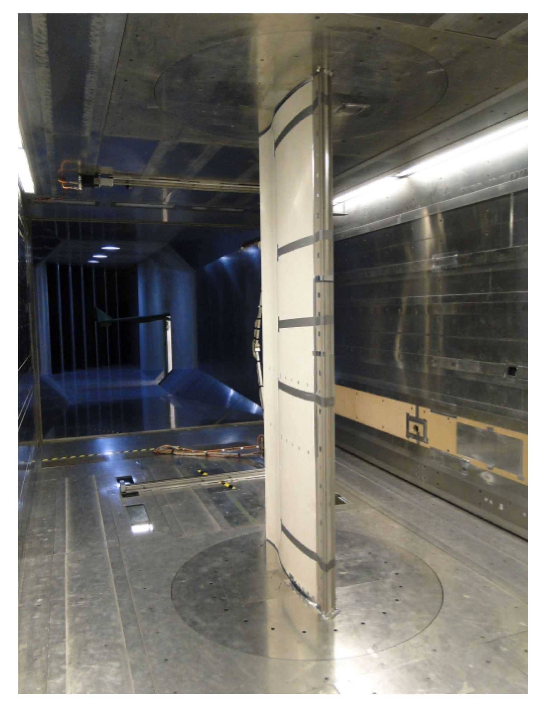
To test the effects of rough, non-aerodynamic ice profiles formed on the leading edge of the wind turbine airfoil, thrown ice bulks were collected from the wind site. Using laser scanning, the 3D shape of the ice bulk was scanned and a 2D section was extracted from it. This 2D section was used to manufacture an extruded section of this 2D profile to be molded to the leading edge of an airfoil as shown in Figure 8. For the airfoil, the tested profile represents a SENVION blade section with thickness to chord ratio ( t / c ) = 20.5 % . This new assembly of the airfoil and molded ice profile are then tested at different Reynolds numbers shown in Table 1.
The airfoil-ice assembly was tested by the German-Dutch wind tunnels (DNW) in the Low Wind Speed Wind tunnel (NWB) located in Braunschweig, Germany [28]. In the experiments used in this work, the open jet section was used, which can hold experiments with wind speeds ranging between 0–80 ms 1 . The test section has a cross-section of 3.25 m × 2.8 m.
Pressure on the surface of the airfoil was measured at 100 different points on the surface of the airfoil using pressure taps distributed over the airfoil’s upper and lower surfaces and the blunt trailing edge.

4.2.2. Case 1: Profile 1 at Re = 2.6 × 10 6

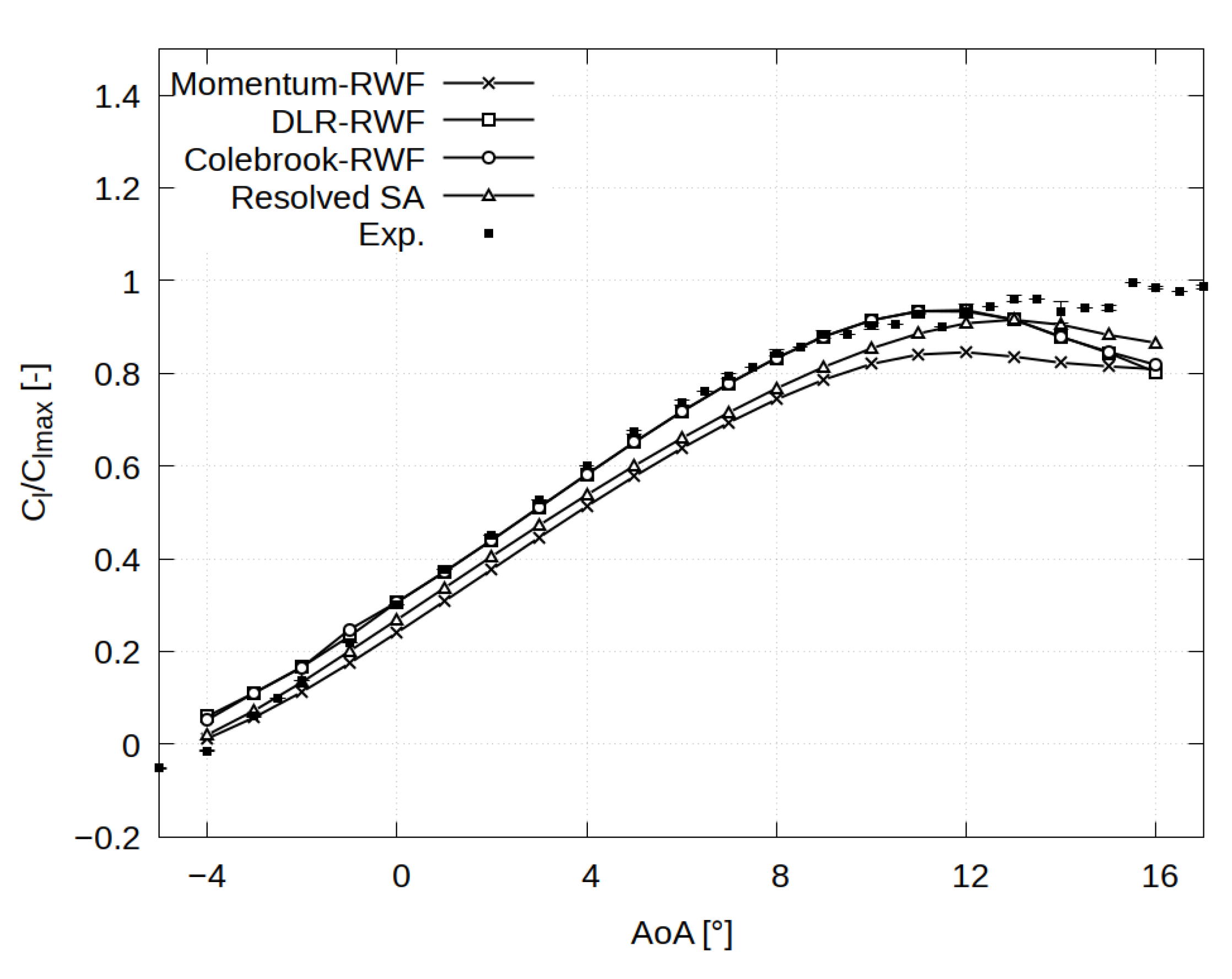
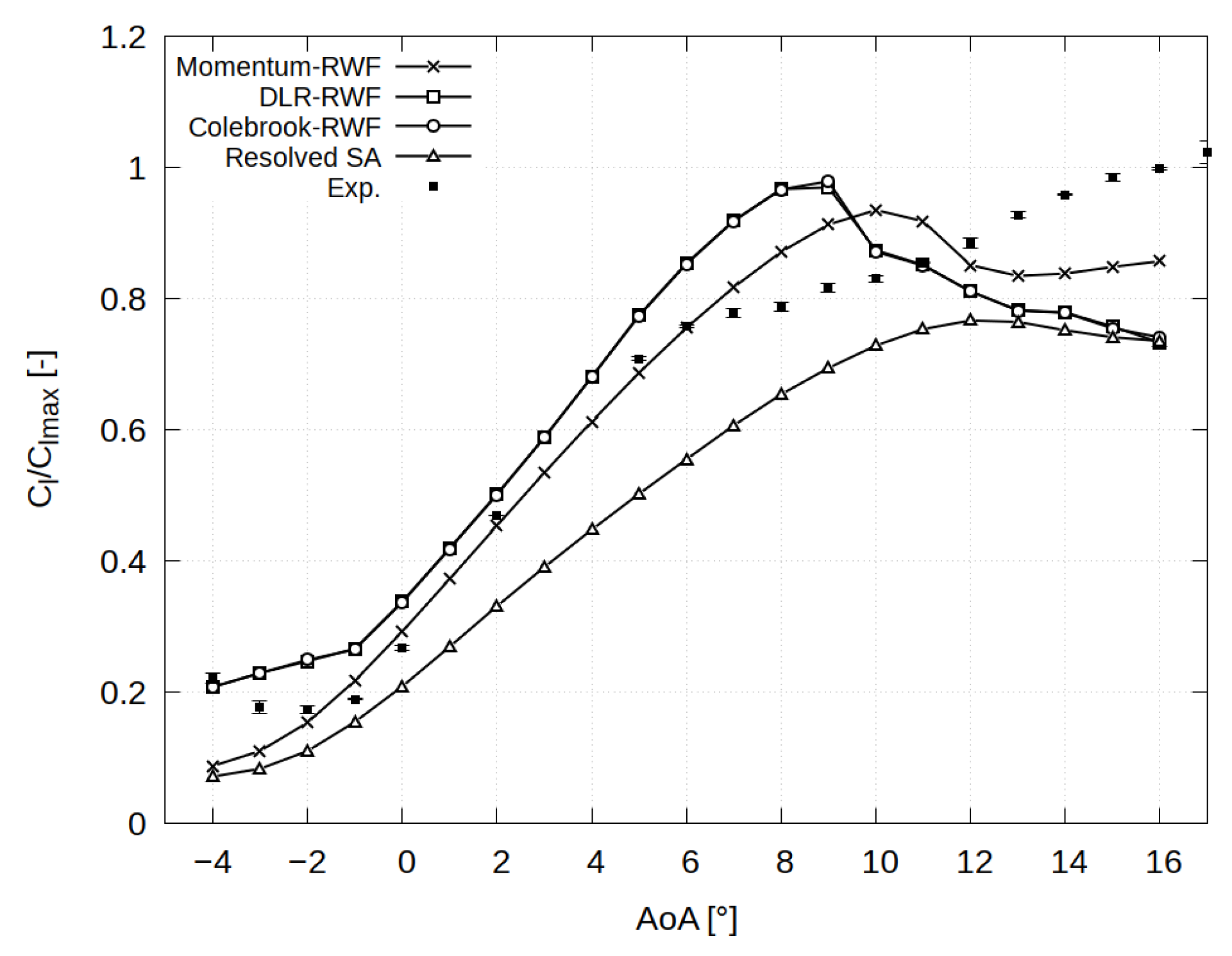
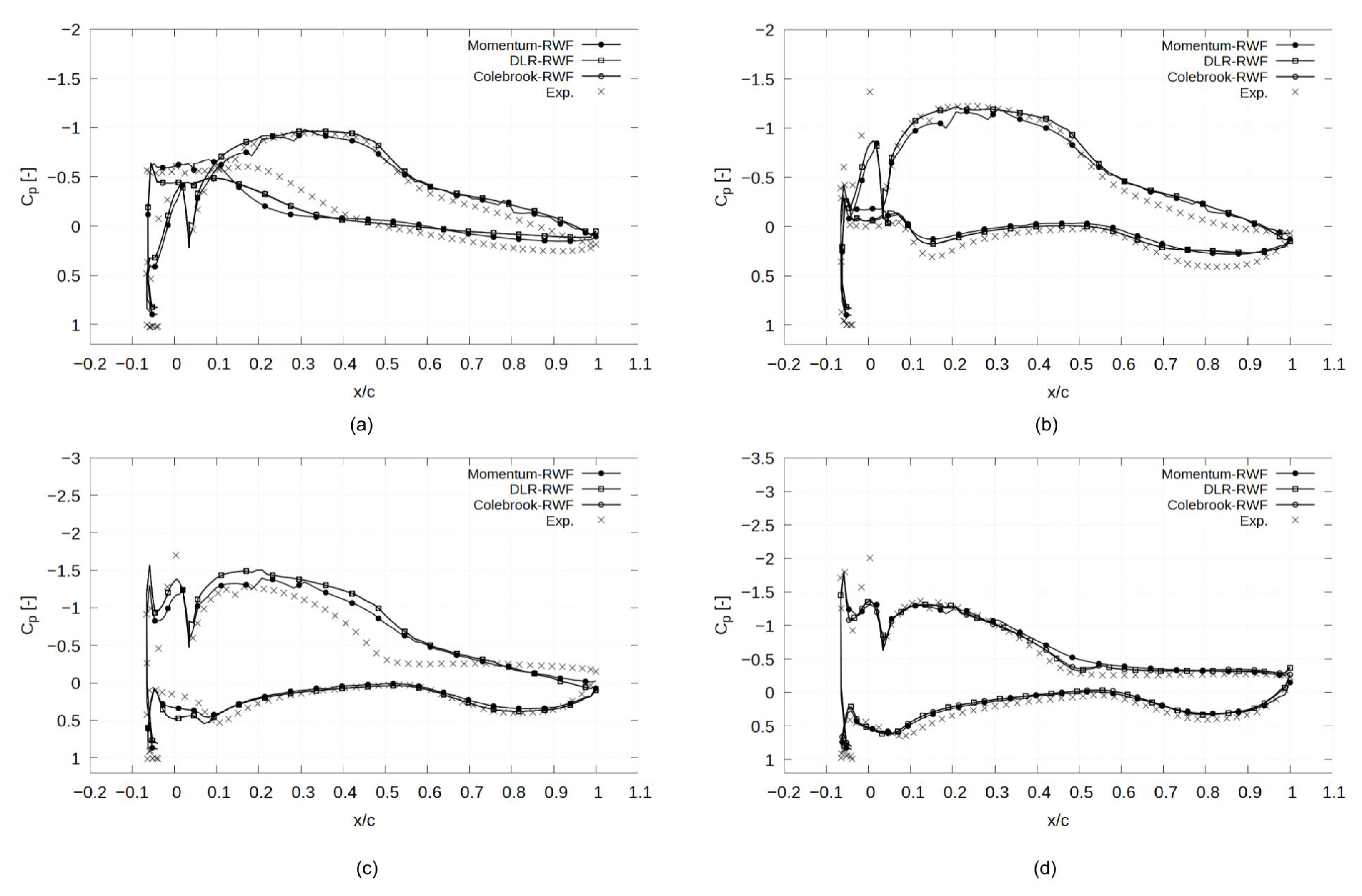
In this case, profile 1 was tested at Re = 2.6 × 10 6 , which is a relatively low Reynolds number compared to the other two cases. Figure 9 shows the comparison between the predictions of each of the three RWFs with wind tunnel results. On the other hand, Figure 10a–d provides a deeper look at the prediction of pressure distribution on the surface of the profile and compares the results with pressure-tap measurement values.
It can be noticed from Figure 9, and also expected, that each model has a different prediction for the maximum lift coefficient C l m a x value or the angle of attack (AoA) at which this C l m a x occurs. However, Momentum-RWF showed the best agreement with C l values. On the other hand, the pressure coefficient ( C p ) shows different behaviors depending on the angle of attack.
Figure 10a–d show that the C p distribution at AoA = 0 , 4 , 8 , and 12 , respectively. At AoA = 0 , a good agreement between experimental and CFD results can be seen except for the lower surface region at x/c ≈−0.05 to 0.05. At AoA’s = 4 and 8 , good agreement was achieved over both smooth and rough surfaces of the airfoil. This agreement starts to suffer from some deviations at AoA = 12 . These deviations are expected due to relatively high AoA that is higher than the AoA of max C l .

4.2.3. Case 2: Profile 1 at Re = 5.1 × 10 6

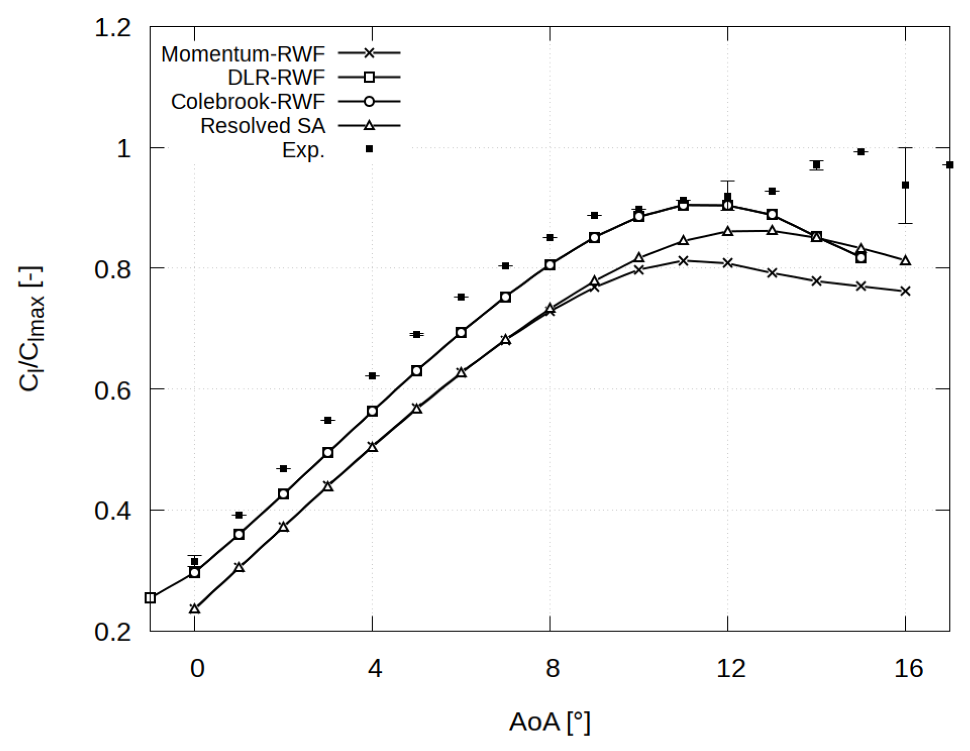
This case is exactly like the previous case except for being tested at Re = 5.1 × 10 6 . This high Reynolds number is challenging for RWFs since it leads to more violent separation and hence is harder to be predicted.
This case shows good agreement (Figure 11), especially in the linear region of AoA vs C l relationship. However, the overprediction of C l m a x can be noticed in DLR and Colebrook RWFs results.
The effect of the high Reynolds number can be seen in C p distribution curves (Figure 12a–d) where large differences between DLR RWF predictions and experimental results occur for AoA = 0 and 4 . In addition, Colebrook RWF shows an underestimation of pressure on the upper surface of the airfoil at AoA = 4 . While the Momentum RWF shows better agreement for all studied AoA’s.

4.2.4. Case 3: Profile 2 at Re = 3.1 × 10 6

In this case, the flow over profile 2 was simulated. It can be noticed from Figure 2 that profile 2 has not only two ice horns, but also it has a rougher surface, i.e., has a higher K s value. The effect of this complex shape can be seen Figure 13. It can be noticed from this figure that the C l curve does not show a clear stall AoA. Only the slope of the C l curve decreases starting from AoA = 5 .
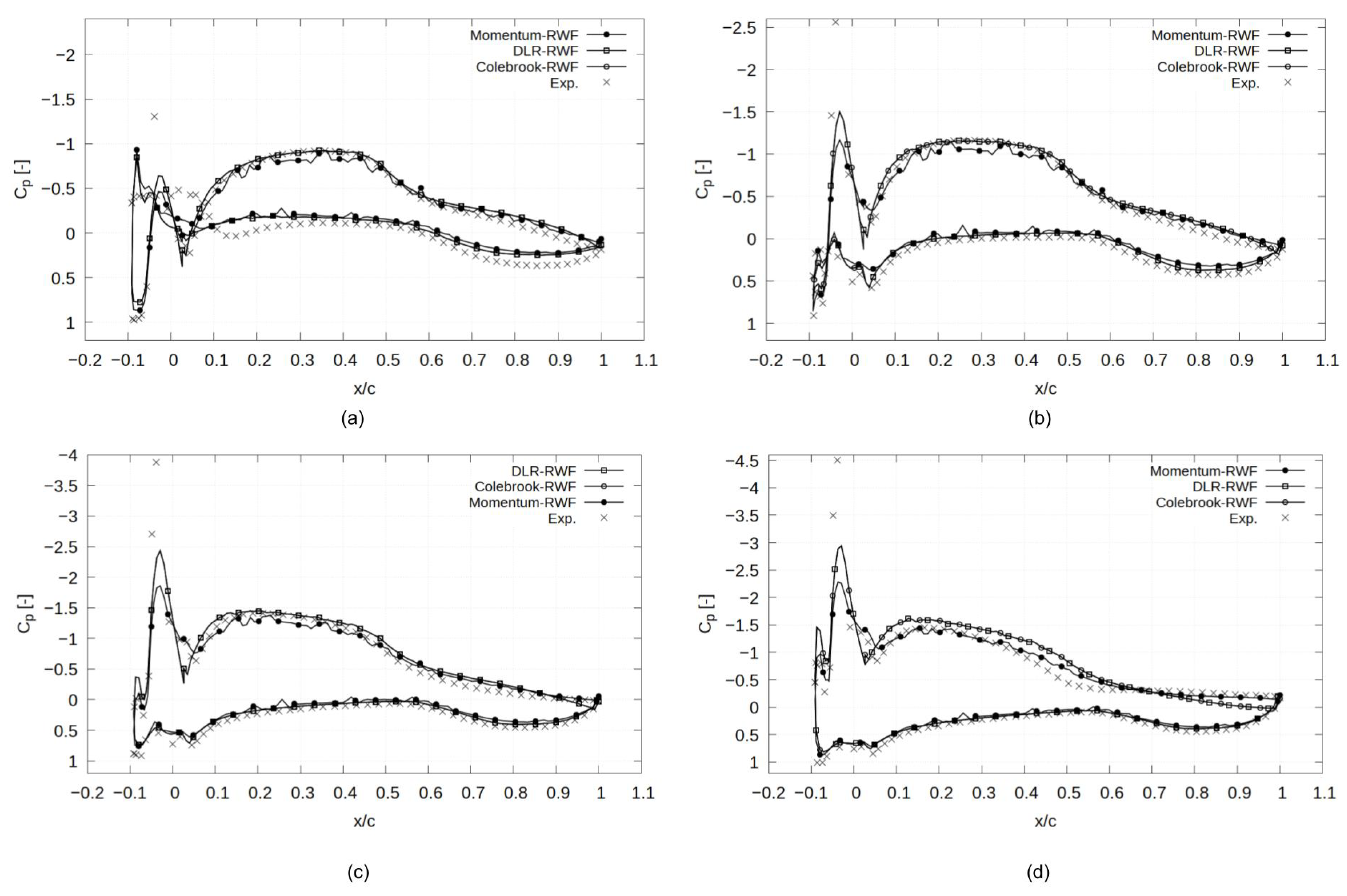
Figure 13 also shows that all compared models had good agreement with experimental results for AoA’s in the range between −1 and 5 . Out of this range, each model shows different behavior. For Colebrook and Momentum RWFs show large deviations from experimental results for AoA’s higher than 5 while DLR RWF shows better agreement in this range. For C p distribution, Figure 14a shows good agreement between the experiment and all simulations at AoA = 0 on the upper surface of the airfoil while they have higher deviations from the experiment on the lower surface in the x/c range between −0.1 to 0.4. At AoA = 4 results shown in Figure 14b, Colebrook and DLR RWFs show large deviations over the whole airfoil while Momentum RWF shows better agreement. In Figure 14c,d good agreement between all models and experimental results can be noticed.

4.3. Analysis of the Agreement between Experiments and RWFs

The results shown in the last sections show that the flow field has different behaviors with using each RWFs. To find out which of the three RWFs resulted in the most accurate results, error analysis should be conducted to find out which RWF had less deviation from the experimental results. C p distribution was chosen as the main criteria to compare since as explained earlier, the C p distribution provides a better understanding of the shape of the flow field over the body which is very important to simulate ice accumulation. In this work, the average absolute error between C p calculated from pressure measurements in the wind tunnel and the corresponding C p calculated from simulations using the standard error of estimates:
σ a v g = 1 N ( C p , e x p C p , s i m ) 2 N
where σ a v g is the standard error, C p , e x p and C p , s i m are coefficients of the pressure of experiments and simulations, respectively, and N is the number of experimental points.
As shown in the Figure 15a,b, it can be noticed that the higher the AoA value, the more error between simulation and wind tunnel results except for some results at AoA = 4 in case 1. While in Figure 15a, we can see that the error values are not increasing with the increase of AoA at the same rates as shown in the previous two figures. These error results show that all RWFs have limited capabilities in simulating the detachment of the flow and accordingly give results deviated from actual results. In addition, in case 3, where profile 2 was simulated, the flow should be highly unsteady which is not suitable for RANS simulations. However, the Momentum RWF managed to predict the C p distribution better than the other models except for AoA = 4 .

5. Discussion and Conclusions

In this work, three different rough wall functions were tested on iced wind turbine airfoils. This comparison aimed to find out which RWF will be the most suitable one to simulate ice accretion on wind turbine blades exposed to icing atmospheric conditions. To be able to apply these RWFs, DLR and Colebrook RWFs were implemented to the OpenFOAM v6 CFD framework along with the existing Momentum RWF. Two ice profiles collected from a wind site, scanned, molded to an airfoil, and tested in the wind tunnel were smoothed by a cubic spline to find the equivalent smooth surface. In addition, roughness parameters described in Section 3.2 were calculated and used to calculate the velocity shift value Δ u .
In this section, general remarks and discussions of the results are introduced. Then the conclusions from the outcomes of this work will be highlighted.

5.1. General Remarks and Discussion

Regarding the rough ice surface shown in Figure 2, one should keep in mind that the ice formation process (or roughness formation in general) is a stochastic phenomenon. This means, that if the same airfoil is exposed to the same atmospheric conditions, the ice profile resulting will not be the same. Hence, to find the real smooth surface required for the simulations, a large number of ice profiles of the same atmospheric conditions should be studied and averaged to find the real average surface. In addition, each rough surface will give different attachment and reattachment bubble locations and might have different overall pressure distribution. However, the scope of this work is only to prove that the RWF approach results in good results compared to experiments.
Figure 16 shows the LIC of flow in cases 2 and 3 at AoA = 0 in a fully resolved grid case only. In the case of coarse grids, such separation bubbles will not be visible since the RWFs compensate for these effects with a mathematical model affecting the different turbulence parameters. From the geometry of the two ice profiles shown in Figure 2, it can be noticed that both profiles are slightly inclined downwards. This inclination forms a relatively big separation bubble behind the profile on the lower surface as shown in Figure 16. That is why we can see deviations between simulations and experimental results of C p distribution in this region (i.e., the lower surface between x/c = −0.1 to 0.1) in most of the studied cases.
It can be noticed from the results that agreement of C l curves between simulations and experimental results does not necessarily mean that the flow field was accurately simulated. For example, in case 3, DLR RWF shows better C l agreement than other models at AoA = 4 while from C p distribution, DLR RWF showed larger deviations from experimental results. The same happened with case 2 at AoA = 0 and 4 . The overall C l at these AoA’s, in the end, had good agreement because the deviations on the upper and lower surfaces compensate for each other which can be misleading in this case. To accurately access the C l , it should be studied together with the C p distribution curves.
It is noteworthy that all the RWFs used are only algebraic equations that express the behavior of the flow near that wall. Accordingly, the three different RWFs have the same computational cost. However, the overall computational cost depends only on the number of cells in the used computational grid and the turbulence model itself as discussed in Section 2.

5.2. Conclusions

In this work, three different RWFs (namely: Momentum, DLR and Colebrook RWFs) are tested using two different rough ice profiles. For each case, C l and C p are compared to experimental wind tunnel results of the lift force and pressure distribution over the airfoil and ice profiles.
The simulation cases show that DLR and Colebrook RWFs provides the best agreement of cases 1 and 2 simulations with experiments compared to the other models. While in case 3, Momentum RWF provides the least errors between experiments and simulations. In some cases, the simulations show fair agreement at locations that witness violent separation such as concave areas between ice and airfoil. This fair agreement is expected due to using steady-state RANS simulations.
Considering that wind turbine airfoils usually operates at AoA’s between AoA = 4 –8 , Colebrook RWF provides the least error between wind tunnel measurements and simulation results in these two AoA’s for the three cases except for case 3 at AoA = 8 . Such a method should be beneficial for the simulation of the performance drop of wind turbine blades exposed to icing atmospheric conditions with minimum computational effort.
Further studies should be conducted to compare the overall performance of wind turbine rotors, power production for instance, after being affected by ice formation on the blades and compare it with measured turbine performance from wind sites.

Author Contributions

K.Y. simulated the cases and wrote the article. H.K. and K.Y. implemented methods in OpenFOAM. T.K. provided experimental data and consultation regarding experimental results. B.S. coordinated the project. B.S. and J.P. provided consultation and supervision. All authors have read and agreed to the published version of the manuscript.

Funding

This work is part of project OptAnIce: Optimales Anti-Icing für Rotorblätter im kalten Klima, funded by the German Federal Ministry for Economic Affairs and Energy (BMWi), fund No.: 0324232C. The simulations were performed using the HPC Cluster EDDY in the University of Oldenburg, a part of WIMS-Cluster project and funded by the BMWi.

Institutional Review Board Statement

Not applicable.

Informed Consent Statement

Not applicable.

Data Availability Statement

The rough ice profiles are available upon request to the corresponding author. The wind tunnel measurements are property of SENVION GmbH and not publicly available.

Acknowledgments

The first author would like to thank the CFD group of Fraunhofer IWES for their discussions and guidance.

Conflicts of Interest

The authors declare no conflict of interest.

Abbreviations

The following abbreviations are used in this manuscript:
A p Area projected normal to streamwise direction
A s Area projected to streamwise direction
Δ B Log-law velocity shift
C l Coefficient of Lift
C l m a x Max lift coefficient
C p Coefficient of pressure
DRoughness element diameter
kTurbulent kinetic energy
KElement Roughness Height
K s Equivalent Sand Roughness Height
LDistance between two roughness elements
u τ Friction velocity
y ( 1 ) First cell height
Abbreviations
RWFRough wall function
RANSReynolds-averaged Navier–Stokes
Greek letters
κ von Karman constant
ω Specific rate of dissipation
ν Eddy viscosity
Subscripts and superscripts
a v g average value
e x p experimental result
s i m simulation result
wwall value
+value in wall scaling

Appendix A. Grid Tests

In this appendix, the process of selecting the suitable first cell height of each profile is shown. To select the first cell height, different values have been tested with the different RWFs to check which cell height provides good convergence of the numerical solution.

Appendix A.1. Grid Tests for Profile 1

In cases 1 and 2, ice profile 1 was simulated at two different Reynolds numbers shown in Table 1. Since the first cell height is dependent only on the roughness height, cases 1 and 2 should have the same first cell height.
From Figure A1, it can be noticed that first cell height y ( 1 ) = 9 mm shows the best stability for the three RWFs
Figure A1. C l vs. AoA of profile 1 for different first cell heights y ( 1 ) using (a) Momentum, (b) DLR, and (c) Colebrook RWF.
Energies 15 08145 g0a1

Appendix A.2. Grid Tests for Profile 2
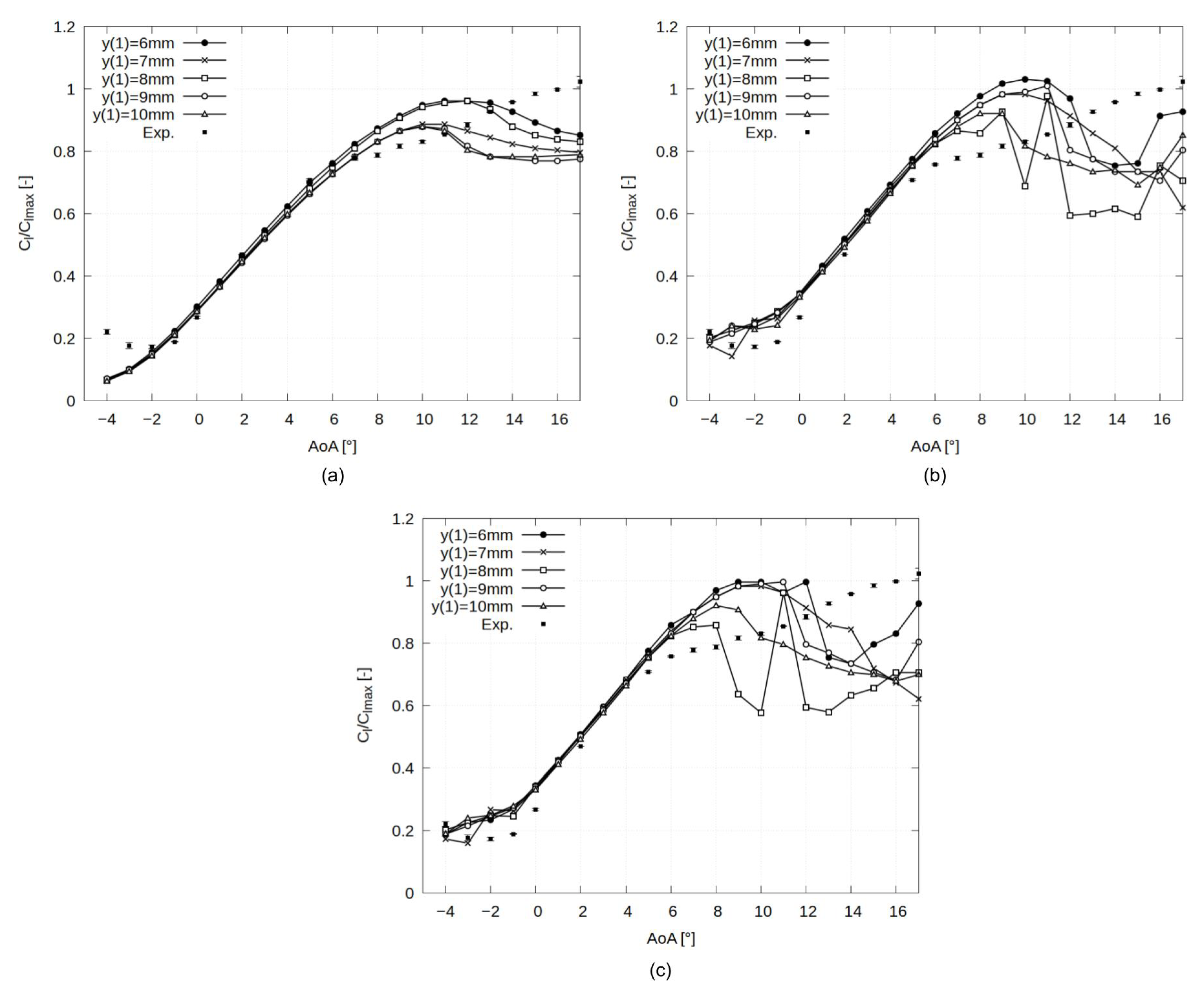
In case 3, where ice profile 2 is simulated. first cell height y ( 1 ) = 10 mm provides the best convergence over the range of simulations.
Figure A2. C l vs. AoA of profile 2 for different first cell heights y ( 1 ) using (a) Momentum, (b) DLR, and (c) Colebrook RWF.
Energies 15 08145 g0a2

References

  1. Sailor, D.J.; Smith, M.; Hart, M. Climate change implications for wind power resources in the Northwest United States. Renew. Energy 2008, 33, 2393–2406. [Google Scholar] [CrossRef]
  2. Nikuradse, J. Strömungsgesetze in Rauhen Rohren. VDI-Forschungsheft, 1933. [Google Scholar]
  3. Schlichting, H. Experimental Investigation of the Problem of Surface Roughness; National Advisory Commitee for Aeronautics: Boston, MA, USA, 1937. [Google Scholar]
  4. Moody, L.F. Friction factors for pipe flow. Trans. Asme 1944, 66, 671–684. [Google Scholar]
  5. Blanchard, A. Analyse Expérimentale et Théorique de la Structure de la Turbulence D’une Couche Limite sur Paroi Rugueuse. Ph.D. Thesis, University of Poitiers, Poitiers, France, 1977. [Google Scholar]
  6. Hosni, M.; Coleman, H.W.; Taylor, R.P. Measurements and calculations of rough-wall heat transfer in the turbulent boundary layer. Int. J. Heat Mass Transf. 1991, 34, 1067–1082. [Google Scholar] [CrossRef]
  7. Hosni, M.; Coleman, H.W.; Garner, J.W.; Taylor, R.P. Roughness element shape effects on heat transfer and skin friction in rough-wall turbulent boundary layers. Int. J. Heat Mass Transf. 1993, 36, 147–153. [Google Scholar] [CrossRef]
  8. Achenbach, E. The effect of surface roughness on the heat transfer from a circular cylinder to the cross flow of air. Int. J. Heat Mass Transf. 1977, 20, 359–369. [Google Scholar] [CrossRef]
  9. Wang, Z.; Zhu, C. Numerical simulation for in-cloud icing of three-dimensional wind turbine blades. Simulation 2018, 94, 31–41. [Google Scholar] [CrossRef] [Green Version]
  10. Chen, H.; Patel, V. Near-wall turbulence models for complex flows including separation. AIAA J. 1988, 26, 641–648. [Google Scholar] [CrossRef]
  11. Hellsten, A.; Laine, S. Extension of the k-omega-SST turbulence model for flows over rough surfaces. In Proceedings of the 22nd Atmospheric Flight Mechanics Conference, New Orleans, LA, USA, 11–13 August 1997; p. 3577. [Google Scholar]
  12. Wilcox, D.C. Turbulence Modeling for CFD; DCW Industries: La Canada, CA, USA, 2006; Volume 3. [Google Scholar]
  13. Da Silva, G.A.L.; Arima, M.N.; Branco, N.N.; de Mattos Pimenta, M. Proposed Wall Function Models for Heat Transfer around a Cylinder with Rough Surface in Cross Flow; SAE Technical Paper; SAE: Warrendale, PA, USA, 2011. [Google Scholar] [CrossRef] [Green Version]
  14. Suga, K.; Craft, T.; Iacovides, H. An analytical wall-function for turbulent flows and heat transfer over rough walls. Int. J. Heat Fluid Flow 2006, 27, 852–866. [Google Scholar] [CrossRef]
  15. Knopp, T.; Eisfeld, B.; Calvo, J.B. A new extension for k–ω turbulence models to account for wall roughness. Int. J. Heat Fluid Flow 2009, 30, 54–65. [Google Scholar] [CrossRef]
  16. Chedevergne, F.; Aupoix, B. Accounting for wall roughness effects in turbulence models: A wall function approach. In Proceedings of the 7th EUCASS Conference, Milan, Italy, 3–6 July 2017. [Google Scholar]
  17. Greenshields, C.J. OpenFoam User Guide; Version 6; OpenFOAM Foundation Ltd.: London, UK, 2017. [Google Scholar]
  18. Versteeg, H.K.; Malalasekera, W. An Introduction to Computational Fluid Dynamics: The Finite Volume Method; Pearson Education: London, UK, 2007. [Google Scholar]
  19. Spalart, P.; Allmaras, S. A one-equation turbulence model for aerodynamic flows. In Proceedings of the 30th Aerospace Sciences Meeting and Exhibit, Reno, NV, USA, 6–9 January 1992; p. 439. [Google Scholar]
  20. Menter, F. Two-equation eddy-viscosity turbulence models for engineering applications. AIAA J. 1994, 32, 1598–1605. [Google Scholar] [CrossRef]
  21. Dirling, J.R. A method for computing rough wall heat transfer rates on reentry nose tips. In Proceedings of the 8th Thermophysics Conference, Palm Springs, CA, USA, 16–18 July 1973; p. 763. [Google Scholar]
  22. Cebeci, T. Analysis of Turbulent Flows with Computer Programs; Elsevier: Amsterdam, The Netherlands, 2004. [Google Scholar]
  23. Aupoix, B.; Spalart, P. Extensions of the Spalart–Allmaras turbulence model to account for wall roughness. Int. J. Heat Fluid Flow 2003, 24, 454–462. [Google Scholar] [CrossRef]
  24. ISO 4287:1997; Geometrical Product Specifications (GPS)-Surface Texture: Profile Method-Terms, Definitions and Surface Texture Parameters. International Organization for Standardization: Berlin, Germany, 2010.
  25. Hawkins, D.M.; Shannon, T.A.; McClain, S.T. Convection from Surfaces with Real Laser-Scanned Ice Accretion Roughness and Different Thermal Conductivities. In Proceedings of the 9th AIAA Atmospheric and Space Environments Conference, Denver, CO, USA, 5–9 June 2017; p. 3579. [Google Scholar]
  26. McClain, S.T.; Vargas, M.M.; Tsao, J.C.; Broeren, A.P. Ice Roughness and Thickness Evolution on a Business Jet Airfoil. In Proceedings of the 2018 Atmospheric and Space Environments Conference, Atlanta, GA, USA, 25–29 June 2018; p. 3014. [Google Scholar]
  27. Liu, X. New near-wall treatment for suspended sediment transport simulations with high Reynolds number turbulence models. J. Hydraul. Eng. 2014, 140, 333–339. [Google Scholar] [CrossRef]
  28. Niedergeschwindigkeits-Windkanal Braunschweig. Available online: https://www.dnw.aero/wind-tunnels/nwb/ (accessed on 12 June 2022).
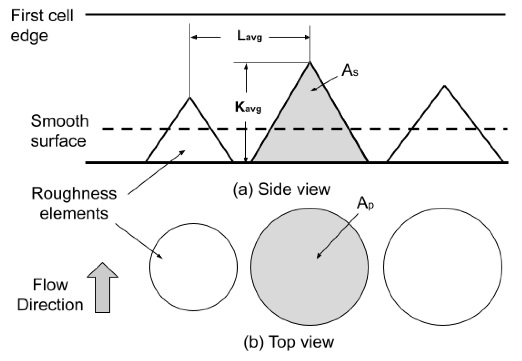
Figure 1. Roughness element geometrical parameters.
Energies 15 08145 g001
Figure 2. Ice profiles 1 and 2.
Energies 15 08145 g002
Figure 3. An example of: (a) smoothing a rough surface using cubic spline and (b) mapping roughness to x-axis.
Energies 15 08145 g003
Figure 4. Comparison between original and smoothed ice surfaces for: (a) profile 1 and (b) profile 2.
Energies 15 08145 g004
Figure 5. Comparison between: (a) fine (with fully resolved roughness) and (b) coarse (with RWFs) grids of profile 1.
Energies 15 08145 g005
Figure 6. Comparison between (a) fine (with fully resolved roughness) and (b) coarse (with RWFs) grids of profile 2.
Energies 15 08145 g006
Figure 7. C p distribution over rough cylinders using implemented wall functions at R e = 4 × 10 6 and: (a) K s = 75 × 10 5 m, (b) K s = 3 × 10 3 m, (c) K s = 9 × 10 3 m where θ = 0 at stagnation point and increases downstream.
Energies 15 08145 g007
Figure 8. Experimental setup of an airfoil with ice profile-1 in the German-Dutch low wind speed, open section wind tunnel.
Energies 15 08145 g008
Figure 9. Case 1: C l vs AoA for different wall functions.
Energies 15 08145 g009
Figure 10. Case 1: C p distribution for AoA = (a) 0 , (b) 4 , (c) 8 , and (d) 12 .
Energies 15 08145 g010
Figure 11. Case 2: C l vs. AoA for different wall functions.
Energies 15 08145 g011
Figure 12. Case 2: C p distribution for AoA = (a) 0 , (b) 4 , (c) 8 , and (d) 12 .
Energies 15 08145 g012
Figure 13. Case 3: C l vs AoA for different wall functions.
Energies 15 08145 g013
Figure 14. Case 3: C p distribution for AoA = (a) 0 , (b) 4 , (c) 8 , and (d) 12 .
Energies 15 08145 g014
Figure 15. Average error between experimental and simulation results of C p distribution (a) case 1, (b) case 2, and (c) case 3.
Energies 15 08145 g015
Figure 16. LIC of flow in (a) case 2 at AoA = 0 (b) case 3 at AoA = 0 .
Energies 15 08145 g016
Table 1. Simulation cases and its grids.
Case No.ProfileAmbient Temp. [ C]ReAoA [ ]y(1) [m]No. of Cells
ResolvedRWFResolvedRWF
1Profile 120.1 2.6 × 10 6 −4 to 16 1.57 × 10 5 9 × 10 3 4.1 × 10 5 7.9 × 10 4
2Profile 127.3 5.2 × 10 6 0 to 16 1.22 × 10 6 9 × 10 3 4.6 × 10 5 7.9 × 10 4
3Profile 220.3 3.1 × 10 6 −4 to 16 1.56 × 10 5 10 × 10 3 4.1 × 10 5 6.3 × 10 4
Publisher’s Note: MDPI stays neutral with regard to jurisdictional claims in published maps and institutional affiliations.