
Deep Learning-Based Methods for Forecasting Brent Crude Oil Return Considering COVID-19 Pandemic Effect

 , , and
Abstract
1. Introduction
2. Literature Review
2.1. Classical Models
2.2. Artificial Intelligence-Based Models
3. Materials and Methods
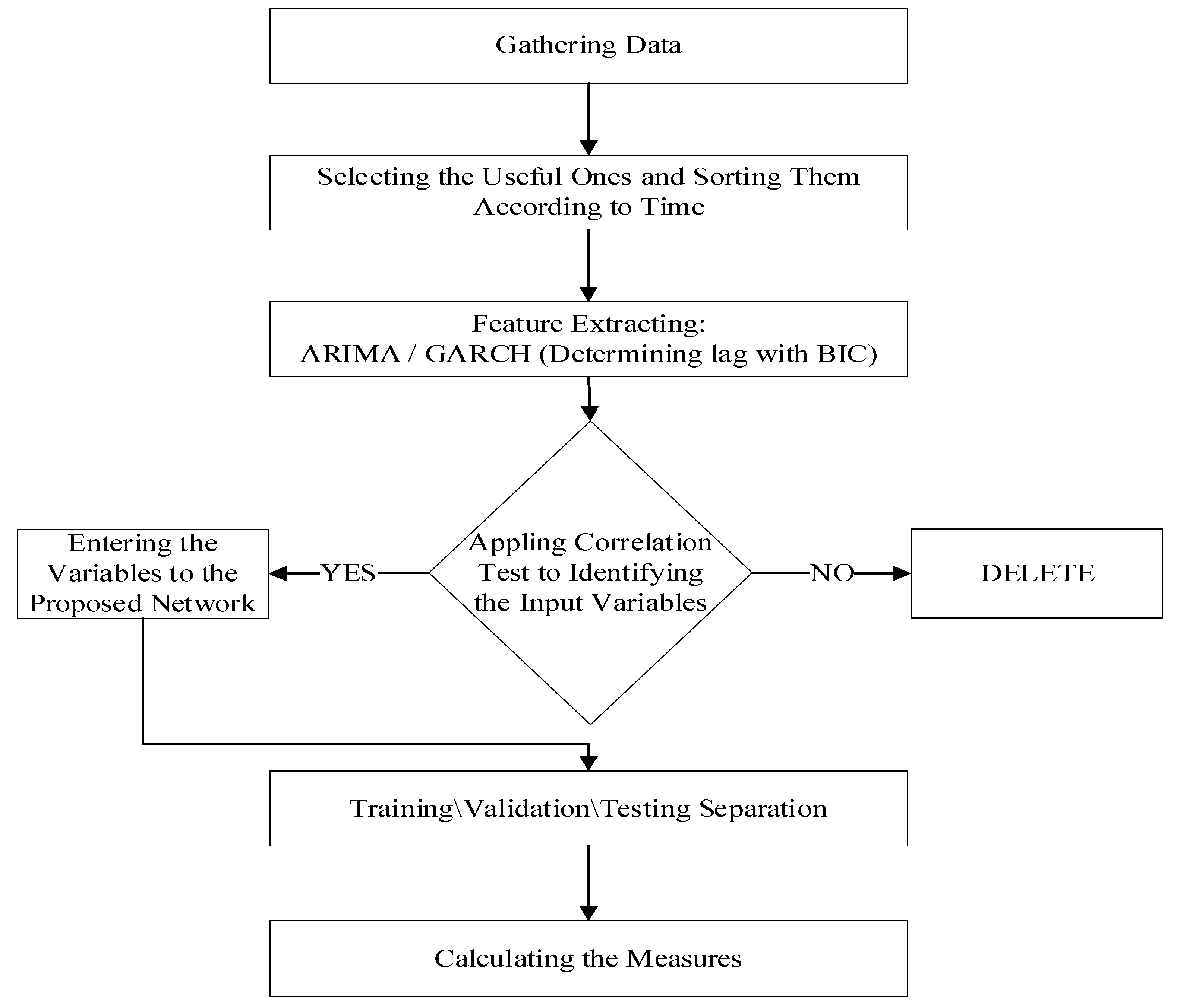
3.1. Methodology
3.1.1. CNN
Convolutional Layers
Max Pooling Layer
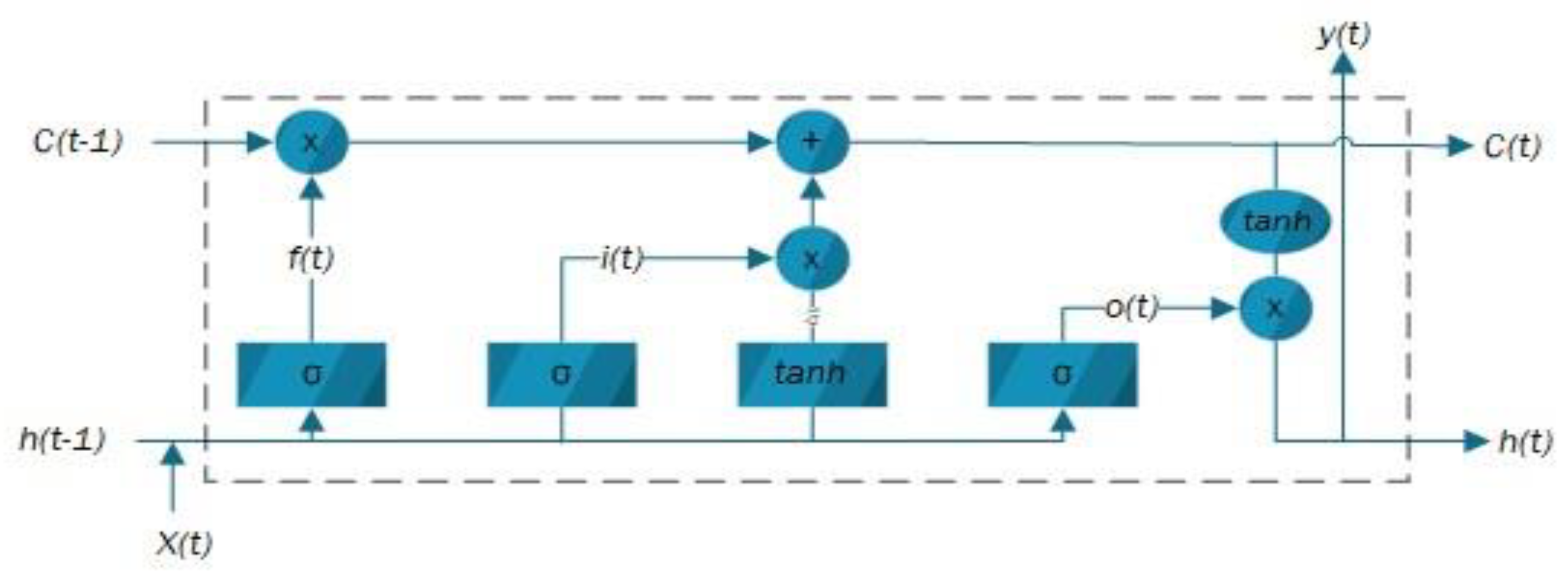
3.1.2. LSTM Model
3.1.3. Trading Strategy
3.2. Comparative and Proposed Models
3.2.1. ANN and ANN-PCA
3.2.2. CNN-ANN and LSTM
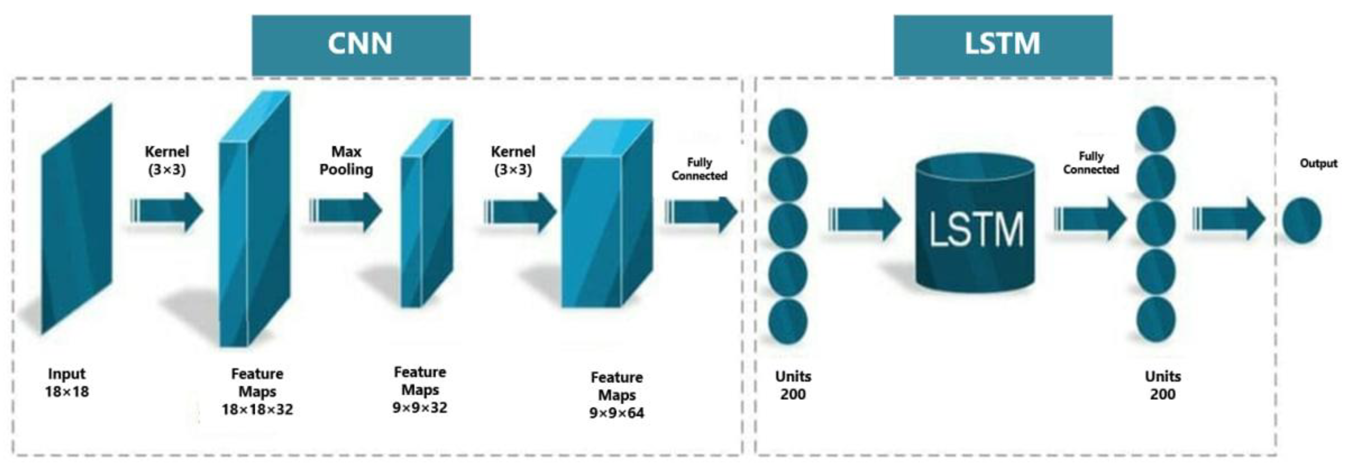
3.2.3. The Proposed 2D CNN-LSTM
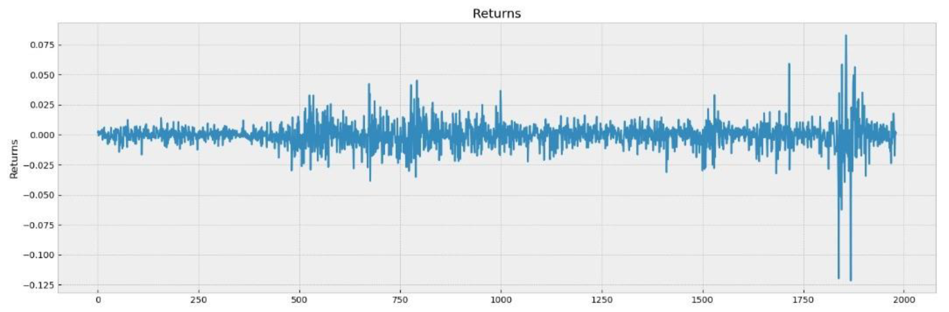
3.3. Characteristics of the Data
3.3.1. Performance Evaluation
Mathematical Tests
Financial Evaluation
4. Results
4.1. Before the COVID-19 Pandemic
4.1.1. Computational Performance Evaluation
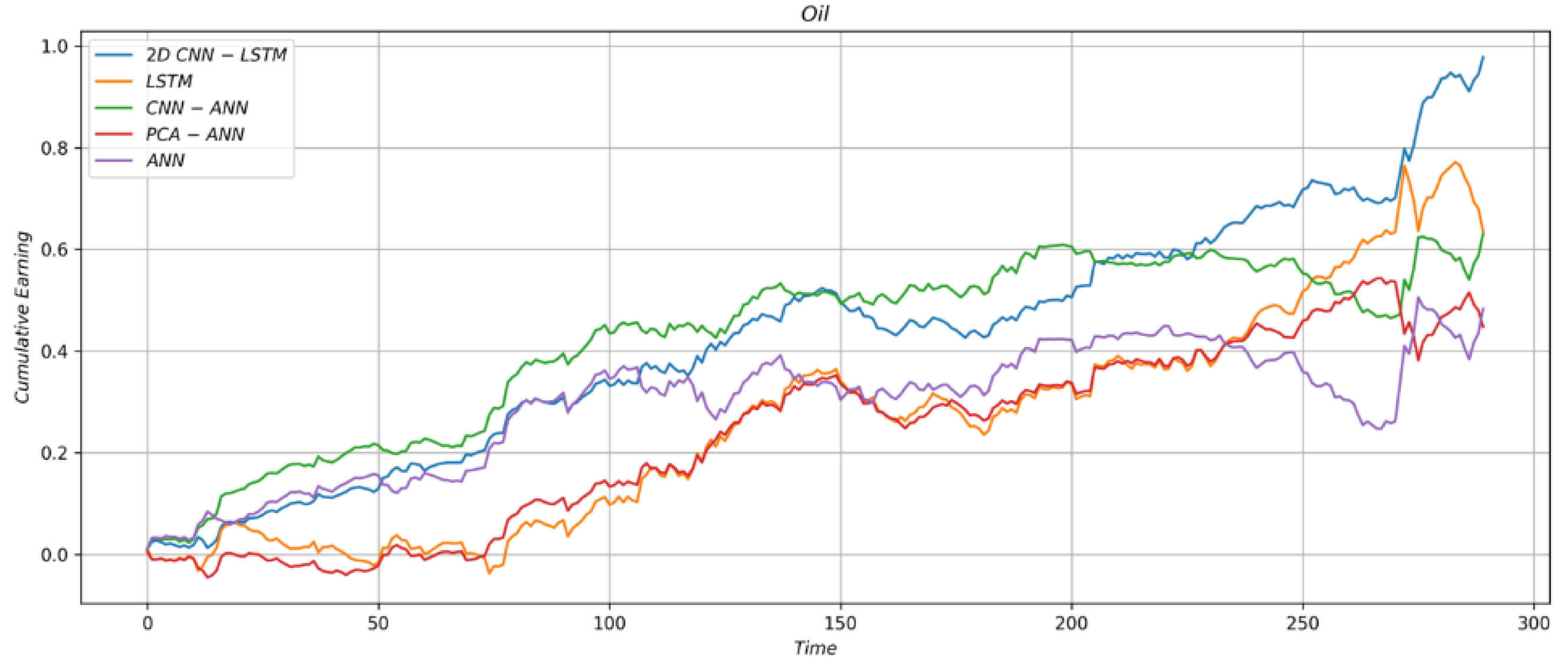
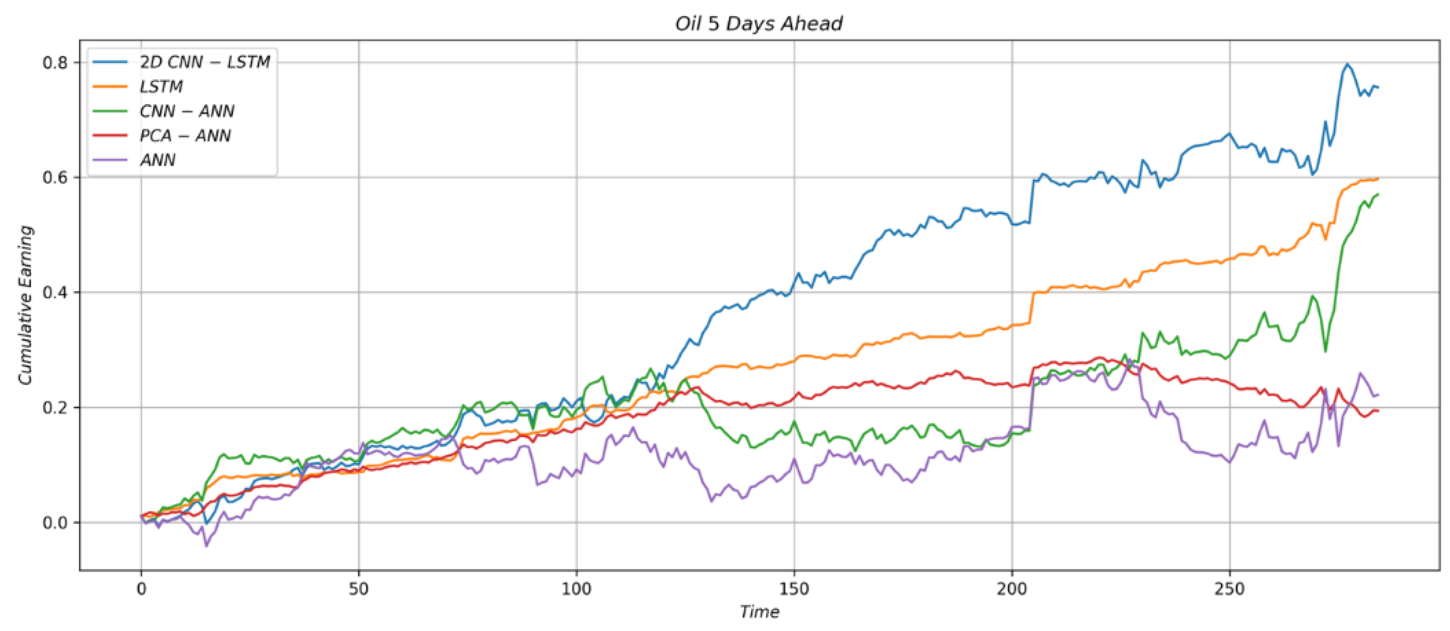
4.1.2. Financial Performance Evaluation
4.1.3. Trading Strategy Results
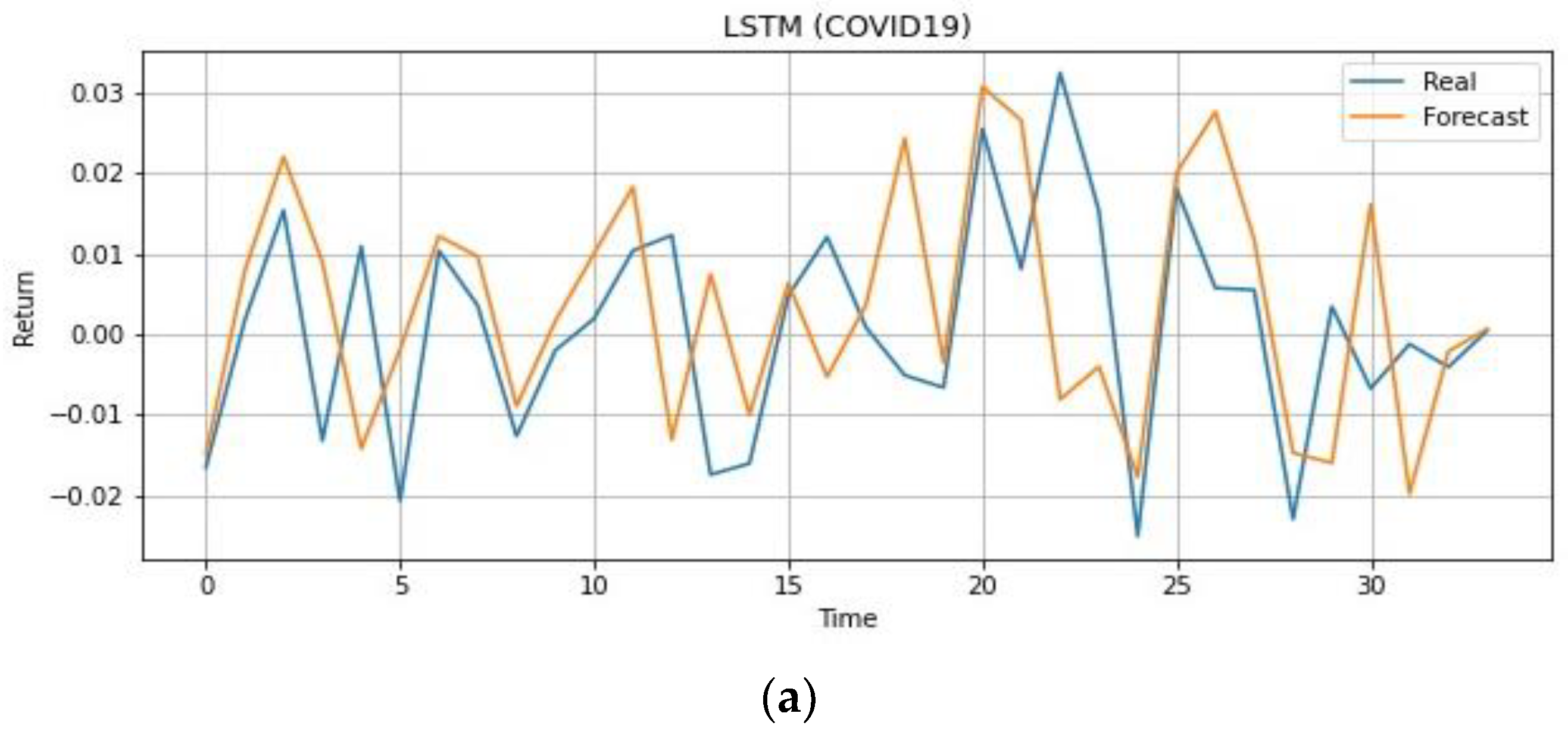
4.2. During COVID-19 Outbreak
5. Conclusions
Author Contributions
Funding
Data Availability Statement
Conflicts of Interest
References
- Deng, S.; Xiang, Y.; Nan, B.; Tian, H.; Sun, Z. A hybrid model of dynamic time wrapping and hidden Markov model for forecasting and trading in crude oil market. Soft Comput. 2020, 24, 6655–6672. [Google Scholar] [CrossRef]
- Quayyoum, S.; Khan, M.H.; Shah, S.Z.A.; Simonetti, B.; Matarazzo, M. Seasonality in crude oil returns. Soft Comput. 2020, 24, 13547–13556. [Google Scholar] [CrossRef]
- Wang, B.; Wang, J. Forecasting hybrid neural network with variational learning rate and q-DSCID synchronization evalua-tion for energy market. Soft Comput. 2020, 24, 16811–16828. [Google Scholar] [CrossRef]
- Zhang, L.; Wang, J. Forecasting global crude oil price fluctuation by novel hybrid E-STERNN model and EMCCS assessment. Soft Comput. 2021, 25, 2647–2663. [Google Scholar] [CrossRef]
- Engle, R.F. Autoregressive Conditional Heteroscedasticity with Estimates of the Variance of United Kingdom Inflation. Econom. J. Econom. Soc. 1982, 50, 987–1007. [Google Scholar] [CrossRef]
- Bollerslev, T. Generalized autoregressive conditional heteroskedasticity. J. Econom. 1986, 31, 307–327. [Google Scholar] [CrossRef]
- Kristjanpoller, W.; Minutolo, M.C. Gold price volatility: A forecasting approach using the Artificial Neural Network–GARCH model. Expert Syst. Appl. 2015, 42, 7245–7251. [Google Scholar] [CrossRef]
- Hajizadeh, E.; Mahootchi, M.; Esfahanipour, A. A new NN-PSO hybrid model for forecasting Euro/Dollar exchange rate volatility. Neural Comput. Appl. 2019, 31, 2063–2071. [Google Scholar] [CrossRef]
- Yu, L.; Wang, S.; Lai, K.K. A neural-network-based nonlinear metamodeling approach to financial time series forecasting. Appl. Soft Comput. 2009, 9, 563–574. [Google Scholar] [CrossRef]
- Lu, Y.K.; Perron, P. Modeling and forecasting stock return volatility using a random level shift model. J. Empir. Finance 2010, 17, 138–156. [Google Scholar] [CrossRef]
- Racine, J. On the nonlinear predictability of stock returns using financial and economic variables. J. Bus. Econ. Stat. 2001, 19, 380–382. [Google Scholar] [CrossRef]
- Hajizadeh, E.; Seifi, A.; Zarandi, M.F.; Turksen, I. A hybrid modeling approach for forecasting the volatility of S&P 500 index return. Expert Syst. Appl. 2012, 39, 431–436. [Google Scholar] [CrossRef]
- Di Persio, L.; Honchar, O. Artificial neural networks architectures for stock price prediction: Comparisons and applications. Int. J. Cir-cuits Syst. Signal Process. 2016, 10, 403–413. [Google Scholar]
- Wu, C.-H.; Lu, C.-C.; Ma, Y.-F.; Lu, R.-S. A New Forecasting Framework for Bitcoin Price with LSTM. In Proceedings of the 2018 IEEE International Conference on Data Mining Workshops (ICDMW), Singapore, 17–20 November 2018. [Google Scholar]
- Karakoyun, E.; Cibikdiken, A. Comparison of ARIMA Time Series Model and LSTM deep Learning Algorithm for Bitcoin Price Forecasting. In Proceedings of the 13th Multidisciplinary Academic Conference in Prague, Prague, Czech Republic, 12–13 October 2018. [Google Scholar]
- Bildirici, M.; Bayazit, N.G.; Ucan, Y. Analyzing Crude Oil Prices under the Impact of COVID-19 by Using LSTARGARCHLSTM. Energies 2020, 13, 2980. [Google Scholar] [CrossRef]
- Dey, P.; Saurabh, K.; Kumar, C.; Pandit, D.; Chaulya, S.K.; Ray, S.K.; Prasad, G.M.; Mandal, S.K. t-SNE and variational auto-encoder with a bi-LSTM neural network-based model for prediction of gas concentration in a sealed-off area of underground coal mines. Soft Comput. 2021, 25, 14183–14207. [Google Scholar] [CrossRef]
- Bollerslev, T.; Chou, R.Y.; Kroner, K.F. ARCH modeling in finance: A review of the theory and empirical evidence. J. Econ. 1992, 52, 5–59. [Google Scholar] [CrossRef]
- Bauwens, L.; Laurent, S.; Rombouts, J.V.K. Multivariate GARCH models: A survey. J. Appl. Econ. 2006, 21, 79–109. [Google Scholar] [CrossRef]
- Lam, K.S.; Tam, L.H. Liquidity and asset pricing: Evidence from the Hong Kong stock market. J. Bank. Finance 2011, 35, 2217–2230. [Google Scholar] [CrossRef]
- Wang, L.; Feng, C.; Song, Q.; Yang, L. Efficient semiparametric garch modeling of financial volatility. Stat. Sin. 2012, 22, 249–270. [Google Scholar] [CrossRef]
- Maciel, L.; Gomide, F.; Ballini, R. Evolving Fuzzy-GARCH Approach for Financial Volatility Modeling and Forecasting. Comput. Econ. 2016, 48, 379–398. [Google Scholar] [CrossRef]
- Sadik, Z.A.; Date, P.M.; Mitra, G. News augmented GARCH(1,1) model for volatility prediction. IMA J. Manag. Math. 2018, 30, 165–185. [Google Scholar] [CrossRef]
- Naimy, V.; Haddad, O.; Fernández-Avilés, G.; El Khoury, R. The predictive capacity of GARCH-type models in measuring the volatil-ity of crypto and world currencies. PLoS ONE 2021, 16, e0245904. [Google Scholar] [CrossRef]
- Hamid, S.A.; Iqbal, Z. Using neural networks for forecasting volatility of S&P 500 Index futures prices. J. Bus. Res. 2004, 57, 1116–1125. [Google Scholar] [CrossRef]
- Pérez-Rodríguez, J.V.; Torra, S.; Andrada-Félix, J. STAR and ANN models: Forecasting performance on the Spanish “Ibex-35” stock index. J. Empir. Financ. 2005, 12, 490–509. [Google Scholar] [CrossRef]
- Wang, Y.-H. Nonlinear neural network forecasting model for stock index option price: Hybrid GJR–GARCH approach. Expert Syst. Appl. 2009, 36, 564–570. [Google Scholar] [CrossRef]
- Bildirici, M.; Ersin, Ö.Ö. Improving forecasts of GARCH family models with the artificial neural networks: An application to the daily returns in Istanbul Stock Exchange. Expert Syst. Appl. 2009, 36, 7355–7362. [Google Scholar] [CrossRef]
- Roh, T.H. Forecasting the volatility of stock price index. Expert Syst. Appl. 2007, 33, 916–922. [Google Scholar] [CrossRef]
- Adhikari, R.; Agrawal, R.K. A combination of artificial neural network and random walk models for financial time series forecasting. Neural Comput. Appl. 2014, 24, 1441–1449. [Google Scholar] [CrossRef]
- Mohammed, G.T.; Aduda, J.A.; Kube, A.O. Improving Forecasts of the EGARCH Model Using Artificial Neural Network and Fuzzy Inference System. J. Math. 2020, 2020, 6871396. [Google Scholar] [CrossRef]
- Tay, F.E.; Cao, L. Application of support vector machines in financial time series forecasting. Omega 2001, 29, 309–317. [Google Scholar] [CrossRef]
- Tang, L.-B.; Tang, L.-X.; Sheng, H.-Y. Forecasting volatility based on wavelet support vector machine. Expert Syst. Appl. 2009, 36, 2901–2909. [Google Scholar] [CrossRef]
- Chen, C.-H.; Yu, W.-C.; Zivot, E. Predicting stock volatility using after-hours information: Evidence from the Nasdaq actively traded stocks. Int. J. Forecast. 2012, 28, 366–383. [Google Scholar] [CrossRef]
- Zhiqiang, G.; Huaiqing, W.; Quan, L. Financial time series forecasting using LPP and SVM optimized by PSO. Soft Comput. 2013, 17, 805–818. [Google Scholar] [CrossRef]
- Geng, L.; Liang, Y.; Zhang, Z.; Shi, X. Forecasting Range Volatility Using Support Vector Machines with Improved PSO Algorithms. Telkomnika 2016, 14, 208. [Google Scholar] [CrossRef]
- Zhao, J.; Mao, X.; Chen, L. Speech emotion recognition using deep 1D & 2D CNN LSTM networks. Biomed. Signal Process. Control 2019, 47, 312–323. [Google Scholar] [CrossRef]
- Lu, C.-J.; Lee, T.-S.; Chiu, C.-C. Financial time series forecasting using independent component analysis and support vector regres-sion. Decis. Support Syst. 2009, 47, 115–125. [Google Scholar] [CrossRef]
- Sun, H.; Yu, B. Forecasting Financial Returns Volatility: A GARCH-SVR Model. Comput. Econ. 2020, 55, 451–471. [Google Scholar] [CrossRef]
- Lawrence, S.; Giles, C.L.; Tsoi, A.C.; Back, A.D. Face recognition: A convolutional neural-network approach. IEEE Trans. Neural Netw. 1997, 8, 98–113. [Google Scholar] [CrossRef]
- Yang, J.; Nguyen, M.N.; San, P.P.; Li, X.; Krishnaswamy, S. Deep Convolutional Neural Networks on Multichannel Time Series for Human Activity Recognition. In Proceedings of the International Joint Conference on Artificial Intelligence, Buenos Aires, Argentina, 25–31 July 2015. [Google Scholar]
- Gunduz, H.; Yaslan, Y.; Cataltepe, Z. Intraday prediction of Borsa Istanbul using convolutional neural networks and feature correlations. Knowl.-Based Syst. 2017, 137, 138–148. [Google Scholar] [CrossRef]
- Hoseinzade, E.; Haratizadeh, S. CNNpred: CNN-based stock market prediction using a diverse set of variables. Expert Syst. Appl. 2019, 129, 273–285. [Google Scholar] [CrossRef]
- Siami-Namini, S.; Tavakoli, N.; Namin, A.S. A Comparison of ARIMA and LSTM in Forecasting Time Series. In Proceedings of the 2018 17th IEEE International Conference on Machine Learning and Applications (ICMLA), Orlando, FL, USA, 17–20 December 2018. [Google Scholar]
- Kim, H.Y.; Won, C.H. Forecasting the volatility of stock price index: A hybrid model integrating LSTM with multiple GARCH-type models. Expert Syst. Appl. 2018, 103, 25–37. [Google Scholar] [CrossRef]
- Cao, J.; Li, Z.; Li, J. Financial time series forecasting model based on CEEMDAN and LSTM. Phys. A Stat. Mech. Appl. 2019, 519, 127–139. [Google Scholar] [CrossRef]
- Tomar, A.; Gupta, N. Prediction for the spread of COVID-19 in India and effectiveness of preventive measures. Sci. Total Environ. 2020, 728, 138762. [Google Scholar] [CrossRef]
- Livieris, I.E.; Pintelas, E.; Pintelas, P. A CNN–LSTM model for gold price time-series forecasting. Neural Comput. Appl. 2020, 32, 17351–17360. [Google Scholar] [CrossRef]
- Krizhevsky, A.; Sutskever, I.; Hinton, G.E. Imagenet classification with deep convolutional neural networks. Adv. Neural Inf. Process. Syst. 2012, 25, 1097–1105. [Google Scholar] [CrossRef]
- Li, W.; Zhu, L.; Shi, Y.; Guo, K.; Cambria, E. User reviews: Sentiment analysis using lexicon integrated two-channel CNN–LSTM family models. Appl. Soft Comput. 2020, 94, 106435. [Google Scholar] [CrossRef]
- Sagheer, A.; Kotb, M. Time series forecasting of petroleum production using deep LSTM recurrent networks. Neurocomputing 2019, 323, 203–213. [Google Scholar] [CrossRef]
- Baek, Y.; Kim, H.Y. ModAugNet: A new forecasting framework for stock market index value with an overfitting prevention LSTM module and a prediction LSTM module. Expert Syst. Appl. 2018, 113, 457–480. [Google Scholar] [CrossRef]
- Abdi, H.; Williams, L.J. Principal component analysis. Wiley Interdiscip. Rev. Comput. Stat. 2010, 2, 433–459. [Google Scholar] [CrossRef]
- Chen, Y.; Hao, Y. Integrating principle component analysis and weighted support vector machine for stock trading signals predic-tion. Neurocomputing 2018, 321, 381–402. [Google Scholar] [CrossRef]
- Zhong, X.; Enke, D. Forecasting daily stock market return using dimensionality reduction. Expert Syst. Appl. 2017, 67, 126–139. [Google Scholar] [CrossRef]
- Haggag, M.; Abdelhay, S.; Mecheter, A.; Gowid, S.; Musharavati, F.; Ghani, S. An Intelligent Hybrid Experimental-Based Deep Learning Algorithm for Tomato-Sorting Controllers. IEEE Access 2019, 7, 106890–106898. [Google Scholar] [CrossRef]
- Hussain, O.K.; Dillon, T.S.; Hussain, F.K.; Chang, E.J. Risk Assessment Phase: Financial Risk Assessment in Business Activities. In Risk Assessment and Management in the Networked Economy; Springer: Berlin/Heidelberg, Germany, 2013; pp. 151–185. [Google Scholar] [CrossRef]
- Sharpe, W.F. Mutual fund performance. J. Bus. 1966, 39, 119–138. [Google Scholar] [CrossRef]
- Khodaee, P.; Esfahanipour, A.; Taheri, H.M. Forecasting turning points in stock price by applying a novel hybrid CNN-LSTM-ResNet model fed by 2D segmented images. Eng. Appl. Artif. Intell. 2022, 116, 105464. [Google Scholar] [CrossRef]
- Bailey, D.H.; de Prado, M.L. Practical Applications of The Deflated Sharpe Ratio: Correcting for Selection Bias, Backtest Overfitting, and Non-Normality. J. Portf. Manag. 2014, 40, 94–107. [Google Scholar] [CrossRef]
- Mohan, V.; Singh, J.G.; Ongsakul, W. Sortino Ratio Based Portfolio Optimization Considering EVs and Renewable Energy in Mi-crogrid Power Market. IEEE Trans. Sustain. Energy 2016, 8, 219–229. [Google Scholar] [CrossRef]
- de Melo Mendes, B.V.; Lavrado, R.C. Implementing and testing the Maximum Drawdown at Risk. Finance Res. Lett. 2017, 22, 95–100. [Google Scholar] [CrossRef]
- Esfahanipour, A.; Khodaee, P. A.; Khodaee, P. A Constrained Portfolio Selection Model Solved by Particle Swarm Optimization Under Different Risk Measures. In Applying Particle Swarm Optimization; Springer: Berlin/Heidelberg, Germany, 2021; pp. 133–153. [Google Scholar] [CrossRef]
- Goodwin, T.H. The information ratio. Financ. Anal. J. 1998, 54, 34–43. [Google Scholar] [CrossRef]
- Szaruga, E.; Kłos-Adamkiewicz, Z.; Gozdek, A.; Załoga, E. Linkages between Energy Delivery and Economic Growth from the Point of View of Sustainable Development and Seaports. Energies 2021, 14, 4255. [Google Scholar] [CrossRef]


| Definition | Symbol |
|---|---|
| The input gate | it |
| The forget gate that controls the previous information | |
| The second gate that controls the new information | Ct∗ |
| The state of memory at the time t | Ct |
| Output gate which manages the information and could be used as the memory cell output | |
| The input | |
| The hidden state that constitutes the memory cell output | |
| Weight matrices | U∗ & W∗ |
| The bias term vectors | B∗ |
| The sigmoid function | σ |
| The component-wise multiplication operator | ʘ |
| Model | Description |
|---|---|
| ANN | Five hidden layers in size order of 200, 150, 120, 80, and 50 neurons Activation function RELU Learning rate 0.01 Batch normalization Cost function MSE |
| PCA-ANN | Five hidden layers in size order of 20, 30, 20, 15, and 10 neurons Activation function RELU Learning rate 0.01 Batch normalization Cost function MSE |
| CNN-ANN | The convolutional layer including 32 filters size (3 × 3) Max pooling layer (2 × 2) The convolutional layer of 64 filters size (3 × 3) Five hidden layers in size order of 200, 150, 120, 80, 50 neurons Activation function RELU Learning rate 0.01 Batch normalization Cost function MSE |
| LSTM | 100 units |
| 2D CNN-LSTM | The convolutional layer including 32 filters of size (3 × 3), max pooling layer (2 × 2) The convolutional layer including 64 filters of size (3 × 3) Fully connected layer with 200 neurons LSTM layer with 100 units |
| Obs. Mean | 1980 −0.0002 |
| Max | 0.0828 |
| Min | −0.1215 |
| Variance | 0.0106 |
| Skewness | −1.0340 |
| Kurtosis | 21.7231 |
| Q2(10) | 6.4905 |
| ARCH test (10) | 26.7749 |
| 1 | Price Normalized | 10 | 8-day lag-return |
| 2 | Return | 11 | 9-day lag-return |
| 3 | 1-day lag-return | 12 | 10-day lag-return |
| 4 | 2-day lag-return | 13 | Index EURO/Dollar |
| 5 | 3-day lag-return | 14 | Price Natural Gas |
| 6 | 4-day lag-return | 15 | US Dollar Index |
| 7 | 5-day lag-return | 16 | Price Crude Oil |
| 8 | 6-day lag-return | 17 | ARIMA(4,0,3) |
| 9 | 7-day lag-return | 18 | GARCH(4,3) |
| Evaluation Criteria | Formula | Descriptions |
|---|---|---|
| MSE | n = number of total iterations each run Av = actual value = forecast value | |
| RMSE | ||
| MAE | ||
| MAPE | ||
| MFE |
| Evaluation Criteria | Description |
|---|---|
| Sharpe Ratio | As a measure of the excess return earned per unit of volatility over the risk-free rate, [58,59] the Sharpe ratio can be determined. |
| Deflated Sharpe Ratio | The deflated Sharpe ratio is used to determine the probability that a discovered strategy is a false positive [60]. |
| Sortino Ratio | In terms of the Sharpe ratio, the Sortino ratio [61] is a variation on this. Sortino calculates the portfolio’s return by dividing it by its downside risk (downside risk refers to the volatility of returns below a certain level, most commonly the average return of the portfolio or returns below zero). The ratio of return generated per unit of the downside risk is represented by Sortino. |
| Maximum Drawdown | A maximum drawdown (MDD) is defined as the maximum loss that a portfolio has experienced between a peak and trough before a new peak is reached. During a specified period, maximum drawdown is an indicator of downside risk [62,63]. |
| Information Ratio | In contrast to the volatility of returns, the information ratio (IR) measures portfolio returns that exceed the returns of a benchmark, usually an index. The benchmark used is usually an index representing the market or a specific sector [64]. |
| Evaluation Criteria | Formula | Description |
|---|---|---|
| Sharpe Ratio | = Expected Portfolio Return = Risk-Free Rate Sigma(p) = Standard Deviation of Portfolio | |
| Deflated Sharpe Ratio | = The expected maximum Sharpe ratio = The estimated Sharpe ratio T = The sample length The skewness of the return’s distribution = The kurtosis of the return’s distribution N = The number of independent trials | |
| Sortino Ratio | Sigma(d) = A measure of the negative asset return’s standard deviation | |
| Maximum Drawdown | LP = Lowest value after peak value PV = Peak value | |
| Information Ratio | = Return’s benchmark rate Tracking error = Excess return standard deviation compared to return’s benchmark rate |
| ANN | PCA-ANN | CNN-ANN | LSTM | 2D CNN-LSTM | |
|---|---|---|---|---|---|
| MSE | 0.0004 | 0.0003 | 0.0003 | 0.0002 | 0.0001 |
| RMSE | 0.0190 | 0.0175 | 0.0173 | 0.0149 | 0.0122 |
| MAE | 0.0146 | 0.0135 | 0.0132 | 0.0050 | 0.0039 |
| MAPE | 2.3440 | 1.4999 | 2.0530 | 0.2070 | 0.1301 |
| MFE | −0.0070 | −0.0078 | 0.0081 | 0.0086 | 0.0017 |
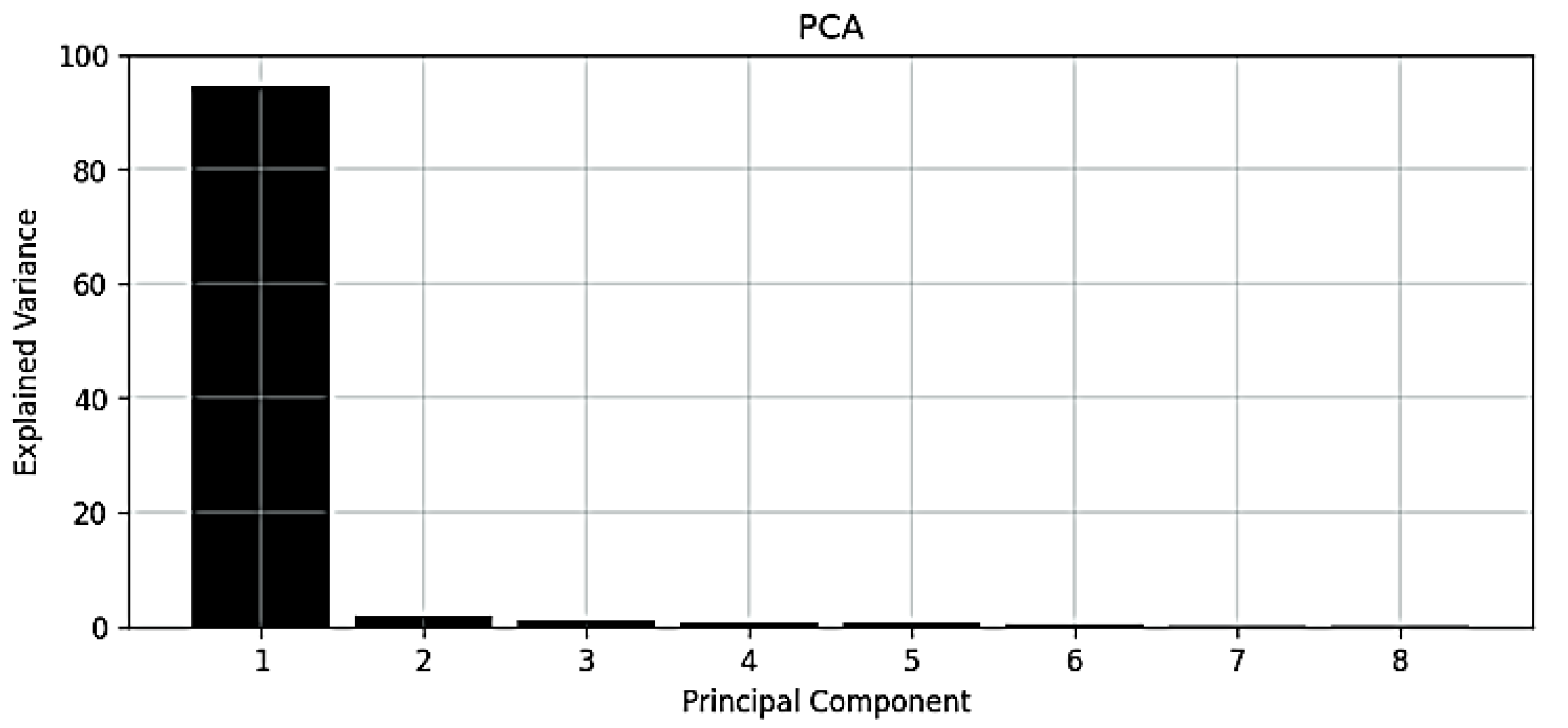
| PCs | Explained Variance | PCs | Explained Variance |
|---|---|---|---|
| 1 | 0.9453 | 10 | 0.0003 |
| 2 | 0.0185 | 11 | 0.0002 |
| 3 | 0.0104 | 12 | 0.0001 |
| 4 | 0.0088 | 13 | 0.0001 |
| 5 | 0.0074 | 14 | 0.0001 |
| 6 | 0.0047 | 15 | 0.0001 |
| 7 | 0.0015 | 16 | 0.0000 |
| 8 | 0.0013 | 17 | 0.0000 |
| 9 | 0.0013 | 18 | 0.0000 |
| ANN | PCA-ANN | CNN-ANN | LSTM | 2D CNN-LSTM | |
|---|---|---|---|---|---|
| MSE | 0.0003 | 0.0003 | 0.0003 | 0.0002 | 0.0001 |
| RMSE | 0.0177 | 0.0177 | 0.0165 | 0.0141 | 0.0119 |
| MAE | 0.0135 | 0.0145 | 0.0066 | 0.0048 | 0.0033 |
| MAPE | 1.5511 | 1.926 | 1.0537 | 0.1495 | 0.1023 |
| MFE | 0.0002 | 0.0022 | 0.0001 | 0.0017 | 0.0010 |
| Model | Mean | Standard Deviation | SE Mean | 95% CI for μ |
|---|---|---|---|---|
| ANN | 0.0007 | 0.0155 | 0.0006 | (−0.0004, 0.0019) |
| PCA-ANN | 0.0020 | 0.0139 | 0.0006 | (0.0008, 0.0031) |
| CNN-ANN | 0.0006 | 0.0055 | 0.0006 | (−0.0005, 0.0018) |
| LSTM | 0.0021 | 0.0063 | 0.0006 | (0.0009, 0.0032) |
| 2D CNN-LSTM | 0.0026 | 0.0130 | 0.0006 | (0.0015, 0.0038) |
| Model | Mean | Standard Deviation | SE Mean | 95% CI for μ |
|---|---|---|---|---|
| ANN | 0.0016 | 0.0141 | 0.0006 | (0.0005, 0.0028) |
| PCA-ANN | 0.0015 | 0.0115 | 0.0006 | (0.0004, 0.0027) |
| CNN-ANN | 0.0021 | 0.0114 | 0.0006 | (0.0010, 0.0033) |
| LSTM | 0.0022 | 0.0150 | 0.0006 | (0.0010, 0.0033) |
| 2D CNN-LSTM | 0.0033 | 0.0111 | 0.0006 | (0.0022, 0.0045) |
| ANN | PCA-ANN | CNN-ANN | LSTM | 2D CNN-LSTM | |
|---|---|---|---|---|---|
| Sharpe Ratio | 0.0808 | 0.0900 | 0.1441 | 0.1110 | 0.2582 |
| Deflated Sharpe Ratio (0.15) | 0.0163 | 0.0340 | 0.1401 | 0.0600 | 0.8801 |
| Deflated Sharpe Ratio (0.2) | 0.0012 | 0.0040 | 0.0204 | 0.0076 | 0.5658 |
| Deflated Sharpe Ratio (0.25) | 0.8620 | 0.8774 | 0.9917 | 0.9439 | 0.9999 |
| Maximum Drawdown | 0.1059 | 0.1038 | 0.0952 | 0.1349 | 0.0764 |
| Sortino Ratio | 0.1268 | 0.1036 | 0.2762 | 0.1637 | 0.5388 |
| Information Ratio (IR) | 0.0737 | 0.0813 | 0.1353 | 0.1043 | 0.2491 |
| ANN | PCA-ANN | CNN-ANN | LSTM | 2D CNN-LSTM | |
|---|---|---|---|---|---|
| Sharpe Ratio | 0.0158 | 0.1062 | 0.0266 | 0.1638 | 0.2501 |
| Deflated Sharpe Ratio (0.15) | 0.0119 | 0.2202 | 0.0183 | 0.5999 | 0.9879 |
| Deflated Sharpe Ratio (0.2) | 0.0010 | 0.0492 | 0.0017 | 0.2546 | 0.8704 |
| Deflated Sharpe Ratio (0.25) | 0.0000 | 0.0056 | 0.0001 | 0.0581 | 0.5012 |
| Maximum Drawdown | 0.1724 | 0.1424 | 0.0524 | 0.1220 | 0.0790 |
| Sortino Ratio | 0.0127 | 0.1554 | 0.0128 | 0.2513 | 0.4005 |
| Information Ratio (IR) | 0.0093 | 0.0990 | 0.0085 | 0.1561 | 0.2341 |
| LSTM (SARS + COVID-19) | LSTM (COVID-19) | |
|---|---|---|
| MSE | 0.0002 | 0.0005 |
| RMSE | 0.0153 | 0.0224 |
| MAE | 0.0110 | 0.0158 |
| MAPE | 2.2044 | 2.7714 |
| MFE | 0.0067 | −0.0056 |
| LSTM (SARS + COVID-19) | LSTM (COVID-19) | |
|---|---|---|
| MSE | 0.0003 | 0.0003 |
| RMSE | 0.0177 | 0.0184 |
| MAE | 0.0145 | 0.0143 |
| MAPE | 1.9260 | 2.8300 |
| MFE | 0.0022 | −0.0001 |
Publisher’s Note: MDPI stays neutral with regard to jurisdictional claims in published maps and institutional affiliations. |
© 2022 by the authors. Licensee MDPI, Basel, Switzerland. This article is an open access article distributed under the terms and conditions of the Creative Commons Attribution (CC BY) license (https://creativecommons.org/licenses/by/4.0/).
Share and Cite
Sajadi, S.M.A.; Khodaee, P.; Hajizadeh, E.; Farhadi, S.; Dastgoshade, S.; Du, B. Deep Learning-Based Methods for Forecasting Brent Crude Oil Return Considering COVID-19 Pandemic Effect. Energies 2022, 15, 8124. https://doi.org/10.3390/en15218124
Sajadi SMA, Khodaee P, Hajizadeh E, Farhadi S, Dastgoshade S, Du B. Deep Learning-Based Methods for Forecasting Brent Crude Oil Return Considering COVID-19 Pandemic Effect. Energies. 2022; 15(21):8124. https://doi.org/10.3390/en15218124
Chicago/Turabian StyleSajadi, Seyed Mehrzad Asaad, Pouya Khodaee, Ehsan Hajizadeh, Sabri Farhadi, Sohaib Dastgoshade, and Bo Du. 2022. "Deep Learning-Based Methods for Forecasting Brent Crude Oil Return Considering COVID-19 Pandemic Effect" Energies 15, no. 21: 8124. https://doi.org/10.3390/en15218124
APA StyleSajadi, S. M. A., Khodaee, P., Hajizadeh, E., Farhadi, S., Dastgoshade, S., & Du, B. (2022). Deep Learning-Based Methods for Forecasting Brent Crude Oil Return Considering COVID-19 Pandemic Effect. Energies, 15(21), 8124. https://doi.org/10.3390/en15218124