Impacts of Trade Friction and Climate Policy on Global Energy Trade Network

Abstract

The trade impacts of the COVID-19 pandemic and the Russian invasion of Ukraine have raised questions about the role of trade and climate policies in energy security and global emissions. This study updates a widely used integrated assessment model (IAM), MESSAGEix-GLOBIOM, to represent complex trade networks to explicitly draw energy flows from their origins to their destination. It then examines the effects of (1) energy trade tariff policies, such as import tariffs, as a proxy to represent an unfriendly trade environment and (2) a global carbon emissions tax on the global energy trade network. Results indicate that trade tariff policies have marginal effects on the trade network, i.e., the size of trade and importing-exporting regions do not change significantly. While high import tariffs significantly reduce emissions due to reduced fossil fuel imports in the importing region, this effect does not translate to significant emission reductions globally, as trade policies only impact downstream of the energy supply chain. However, a carbon emission tax dramatically alters the trade network, by (1) reducing its size by up to 50% and (2) forming trade linkages that allow for a more complex and diverse network of suppliers. This diversity under the emissions tax scenario improves the energy security of major energy-importing regions. Moreover, under an emission tax scenario, a friendly trade environment reduces the energy system costs globally. However, trade friction, such as sanctions or high import tariffs, will increase the energy supply cost significantly, especially for energy-importing regions such as Europe, East and South Asia.

1. Introduction

1.1. Background

Large-scale energy transitions are required to meet the commitments put forth in the Paris Climate Agreement [1,2]. Global assessments provide direction to international policymaking and target setting via nationally determined contributions (INDC) [3]. Region-specific analyses are used to test the feasibility and impact of these transitions because the system requirements of one region do not translate to another [4,5]. However, a region’s energy system not only depends on its own production and consumption of energy, but also the ways in which it interacts with others [6]. These interconnections form a robust trade network [7,8], and the dynamics of this network (i.e., the rate at which trade interconnections form, grow, constrain, and break) inform the rate at which new energy technologies can be adopted.

Recent events underscore the need to better understand the linkages among trade, policy, and energy use. COVID-19 posed a major shock to global supply chains. This was particularly pronounced in the global semiconductor shortage, which cascaded throughout consumer technology and automobile supply chains. This type of unforeseen shock can severely limit the rate at which clean energy technologies, which often rely on many different inputs from many different countries, can diffuse through the global market. The Russian invasion of Ukraine poses yet another direct shock to the global energy trade network. In July 2022, Gazprom, Russia’s main gas company, threatened to cut its gas supply to the EU [9]. Notably, 83% of the EU’s gas consumption came from imports in 2021 [10]. While this type of shock can have the effect of accelerating the EU’s transition to clean energy resources [11], it can also cause other regions to ramp up their gas production to fill the gap that Russia left [12]. It is now clear that we need a better way to model these types of shocks and their implications for advancing climate policy.

1.2. Literature Review

Existing literature suggests that climate policies, such as emissions taxes or cap-and-trade schemes, may have a large impact on international energy markets [13]. Recent literature also suggests that the reverse is not necessarily true; trade policy may not have as large an impact on emissions reduction as previously assumed [14,15]. For this line of research, Integrated Assessment Models (IAMs) are often used to assess the complex interconnections between economic processes (e.g., demand of oil) and physical processes (e.g., carbon emissions). IAMs allow for a coherent analysis of disparate fields in environmental research, including economics, demography, atmospheric chemistry, oceanography, and ecology. Because of this wide disciplinary scope, each IAM makes explicit assumptions on how global systems operate. As such, a group of IAMs (e.g., AIM [16], MESSAGE [17], IMAGE [18]) are used collectively to frame policy evaluations, such as the scenarios used by Intergovernmental Panel for Climate Change (IPCC) reports [19].

In addition to its interactions with climate policymaking, the global energy trade network plays a key role in determining energy security [20]. The conventional approach to achieving energy security is by diversifying the trade portfolio; energy importers are considered less vulnerable when they import more diverse types of resources from a greater number of exporters [21]. Energy independence, or the ability to meet the national energy demand using only domestic resources, is also used as a key indicator for energy security [15,22]. In the last few decades, energy security indices have been updated so that they also address issues of geopolitical path dependence [23,24], energy shocks (e.g., the oil shock of the 1970s, the COVID-19 pandemic [25], and the Russia–Ukraine war in 2022 [26]), and the integration of new economies into the global market [21].

Despite advances in both energy security research and IAMs, few studies have examined the role of trade networks in projections of global energy pathways. Extensive literature exists on historical networks of energy flows, both in terms of physical fuels and the energy embodied in goods and services. For the former, researchers can rely on bilateral trade data to visualize the fuel trade as a network [8,27]. For the latter, input–output analysis (IOA) can be used to estimate the energy required to produce a good or render a service [28,29]. While these retrospective analyses describe how the current global energy network came to be, they cannot be used to forecast possible energy networks of the future. First, regions have heterogenous responses to economic and policy events based on their natural resources, demographics, political economy, and geography. In addition, methods such as IOA are static models that provide snapshots of the global system. A time series built from multiple years of IO tables would be similar to stringing together a series of snapshots without an understanding of how one system evolved into another. These methods are therefore inappropriate for modeling the future global trade network. Second, large-scale, optimization-based, global energy models that provide trajectories of energy use and emissions have not evaluated energy trade as a network problem. They focus on energy stocks and flows by region, rather than the energy stocks and flows between regions. However, economic and political linkages among countries underpin international policymaking. Understanding how these linkages might evolve is crucial in developing effective policy.

1.3. Contribution of This Study

In this study, we bridge the gap between global energy models and trade network analysis by introducing and applying a framework for modeling bilateral trade in MESSAGEix [17,30], which is the core of the MESSAGEix-GLOBIOM integrated assessment framework, one of several key global energy-land use models. MESSAGEix is an optimization-based model, in which the objective function is to minimize global energy system costs. This minimization mimics decision making by each region. The most disaggregated specification to date represents the world in 14 regions. We use this specification to explicitly model trade flows between regions, which allows us to represent global energy trade as a network. We then use this framework to answer two key questions for the nexus of climate and trade policymaking.

We first analyze the emissions and energy security consequences of trade policy. Here, we focus on tariff policies and model three scenarios: a baseline tariff scenario in which rates are held at the historic median by importers, a low tariff scenario in which rates are removed by 2030, and a high tariff scenario in which historic median rates are increased by a factor of five by 2030 (here, we use the word “rate” interchangeably with ad valorem equivalent (AVE) rates for energy commodities). This reflects the upper bound on regional fluctuations in historic tariff rates. We estimate the effect of tariffs on emissions and examine whether these policies, taken independently, can reduce or increase global and regional emissions. We also explore the effects of these policies on energy security by using complex network analysis (CNA) metrics to assess the stability of the trade network and measuring the diversity and dependence of each region’s energy trade portfolio. Note that, throughout the paper, we will use the term “trade” to mean the trade of energy resources (for the purposes of this study, we focus solely on the trade of physical energy resources and not on the energy that is embodied in goods and services).

Second, we analyze the trade and energy security consequences of climate policy. In this study, we represent climate policies through a global tax on greenhouse gas emissions. Emissions taxes are a widely discussed tool for emissions reduction and their potential consequences have been extensively studied using general equilibrium models [31,32], statistical analysis [33,34], and IAMs. We build on this literature by using MESSAGEix to model the effect of a global $27/tCO₂ ($100/tC) emissions tax in 2020 that increases by 5% each year. We model the effect of this tax on the global energy trade network to 2050. We then apply the same metrics as in the first question to assess global emissions, network stability, and regional energy security. Further, we model the low/high tariff scenarios under a carbon emissions tax to examine the marginal effect of trade policy in the presence of a strong climate policy. For the rest of this paper, we use the term emissions tax interchangeably with a carbon emissions tax.

Through these two questions, we hope to (i) better understand how these two policies diverge in their impacts on the global energy trade network, and (ii) estimate the impacts of these policies’ interaction. Our results suggest that tariff policies have little impact on the size and composition of the global energy trade network in 2050. Emissions taxes, on the other hand, systematically change the types of energy that are traded and how this trade is conducted. We observe three types of changes under this policy. First, the network shifts from trading primarily crude oil to primarily trading light oil. As a refined petroleum product, light oil commands a higher price than crude oil. The reason that we observe this change is that the cost of importing a fuel with a high emissions factor (e.g., coal, crude) is greater than the cost of importing a more expensive fuel that has a lower emissions factor. Second, the trade network becomes more complex under an emissions tax scenario. Large energy linkages that exist in the baseline scenario are broken down into smaller linkages, each carrying a smaller amount of fuel. Finally, under an emissions tax scenario, the size of the network contracts significantly (~50%). Unsurprisingly, the emissions tax has a much more substantial impact on global emissions than trade tariffs. While a high tariff policy reduces emissions that are directly linked to imports, its impacts on overall emissions are minimal. The impacts of a tariff policy on energy security metrics are limited. On the other hand, an emissions tax, because it generates more linkages among regions, increases the energy security of key importers.

We begin this paper by introducing the data used to support the bilateral trade framework in MESSAGEix and our scenario analysis. We then present the methodology for this study, including a brief introduction to MESSAGEix, the conceptual framework for the bilateral trade representation, additional developments to MESSAGEix required to support this representation, and scenario design. Finally, we discuss the results of the model and their implications for energy security and climate change mitigation.

2. Materials and Methods

2.1. Configuring Bilateral Trade in MESSAGEix

MESSAGE is a dynamic linear least-cost optimization model that is developed and maintained at the International Institute for Applied Systems Analysis (IIASA) for the purpose of modeling energy system decision making and the associated environmental impacts. The model, developed over four decades, hinges on an objective function that minimizes the total system cost (i.e., the total cost of meeting the energy demand across all regions) while being subject to dozens of economic and physical constraints [35]. MESSAGE has been used extensively in international climate policy, including in the assessment reports published by the Intergovernmental Panel on Climate Change (IPCC) [36]. MESSAGEix is a recent, open-source iteration, developed for the purposes of increasing transparency and efficiency in data compilation and use across scenarios [17]. MESSAGEix provides a flexible model structure; researchers can apply their own data platform to implement the model at any geographic level. This study uses MESSAGEix in combination with the ixmp platform, a database that includes historical data on global energy use patterns, shared socioeconomic pathways, and associated parameter assumptions. Most recently, MESSAGEix has been used to understand electricity sector reliability [37], as well as the implications of increasing energy efficiency in industry [38,39].

MESSAGEix currently represents the world through 14 regions. A table of represented countries and their corresponding regions can be found in the Supplementary Materials. For the purposes of this analysis, we set these 14 regions as the nodes in our trade network. Trade, with the exception of gas interconnections in Europe, is represented through what we call the global pool schema in MESSAGEix. In this schema, regions with excess energy resources can export to a global pool from which regions that demand this resource can import. Figure 1a below illustrates the global pool schema as a map. Figure 1b represents the same schema as the flow of energy from one region to another. Here, commodities represent a specific energy resource (e.g., LNG) while technologies represent the movement of the commodity (e.g., LNG exports, LNG imports). The technology is differentiated by commodity but not by location. This is what defines the global pool schema. Note that while the global pool schema allows us to examine the total exports from/imports to regions, it does not explicitly model the trade flows among them. This explicit bilateral representation is necessary to model trade as a network and to measure security indices such as trade portfolio diversity and import dependence.

The bilateral trade representation is illustrated in Figure 1c,d. To explicitly delineate bilateral trade flows among regions, we needed to completely reparametrize trade in MESSAGEix.

Note that in the global pool schema, the origin of fuel imports and the destination of fuel exports are not explicit in the commodity or technology. In the bilateral framework, we explicitly define the destination of commodity imports (e.g., LNG_weu means LNG imports to Western Europe) and export technologies (e.g., LNG_exp_weu means LNG exports from the given region that are destined for Western Europe). This is illustrated in Figure 2.

For this analysis, we focus on eight commodities: coal, crude oil, ethanol, fuel oil, light oil, liquid hydrogen, LNG, and methanol. We use the BACI bilateral trade database from CEPII to extract historical bilateral trade activity at the region level for each commodity [40]. BACI includes bilateral trade flows of products in both monetary units ($1000) and weight (tons). The data are identified at the importer–exporter–product–year level, and span from 1995 to 2018. In

Table 1. Interregional trade in key fuels (2018). Energy flows are derived from the BACI bilateral trade database, which includes the value and tonnage of trade between countries at the HS6 level. We then convert trade flows from tonnage to EJ using specific energy values published by the IEA.

Commodity	Total Trade (EJ)	Largest Interregional Flows
Coal	19.35	Pacific OECD to South Asia (3.51 EJ) Pacific Asia to Centrally Planned Asia (3.51 EJ) Pacific OECD to Centrally Planned Asia (3.07 EJ)
Crude oil	53.20	Middle East to Centrally Planned Asia (9.79 EJ) Middle East to South Asia (6.69 EJ) Middle East to Western Europe (6.55 EJ)
Fuel oil	17.50	Western Europe to Middle East (1.35 EJ) Middle East to Western Europe (1.31 EJ) Middle East to Pacific Asia (1.09 EJ)
LNG	13.01	Middle East to Western Europe (2.32 EJ) Central Asian States to Centrally Planned Asia (1.53 EJ) Middle East to South Asia (1.43 EJ)

, below, we illustrate the total amount exported/imported for each fuel type among the 14 regions represented in MESSAGE in 2018. This table was built by aggregating BACI data to the region level and converting interregional flows from weight (ton) to physical values (EJ) using IEA conversion values (the correspondence between countries and the 14 MESSAGE regions can be found in Table S3 in the Supplementary Materials). The regional flows are aggregated based on the national flows in each region, according to the mapping presented in Table S3 in the Supplementary Materials.

To calibrate the trade flows derived from the BACI database, we link these data with the Net Calorific Value (NCV) dataset from the International Energy Agency (IEA), which includes data on the energy content (in kJ/kg) of energy resources at the country–year level (our aggregation methodology for both the BACI and NCV datasets is presented in Section 2 in the Supplementary Materials). We use the NCV data to convert units on bilateral trade flows from weight to energy. We then benchmark these data against the World Energy Balances (WEB) database from the IEA. The WEB has total imports and exports of energy resources from individual countries but does not represent these amounts bilaterally.

Trade under the global pool schema utilizes 22 parameters. Parameters are user-defined values that build constraints and costs for the optimization model. One example of a parameter is the emissions factor, which defines the per unit emission by an energy technology (e.g., coal power plants). Another one is the upper bound on the growth constraint for activity; this parameter sets an upper limit for how much more a technology can be adopted compared to the previous timestep. The parameters used in the global schema are presented in Table S4 in the Supplementary Materials. The bilateral trade framework takes each of these parameters and applies them to each trade technology, now differentiated by region.

A key assumption underlying the global pool schema is that the characteristics, and therefore the costs, of maritime shipping are equal across energy commodities. This is clearly not a realistic assumption; for instance, the vessels that carry LNG are vastly different from the vessels that carry coal. To address the heterogeneity across shipping capacity and to ensure that trade growth does not outpace the growth of the global capacity for maritime shipping, we include additional constraints for fuel shipping. Details on these constraints can be found in Section 8 in the Supplementary Materials.

2.2. The Effect of Sea Distance on Trade Cost

In the bilateral representation of energy trade, we assume that—all else being equal, and in the absence of any sanctions or other constraints—exporters are more likely to trade with regions that are closer to them. This is based on the gravity model of bilateral trade, which assumes that trade flows are a function of the size of each economy and the distance between them [41]. To represent the trade friction from distance, we therefore need to estimate the marginal effect of distance on trade cost. Because the objective function in MESSAGEix is to minimize costs, by incorporating trade frictions through the exporting region’s variable cost, we can capture the impedances to trade flows.

We apply a regression analysis using data from the U.S. International Trade Commission (USITC) that are linked to the BACI data introduced above. The USITC data include information on importer and exporter GDP, population, and a slew of relative variables that can introduce or reduce trade friction. We develop the distance-based variable cost term by: (1) measuring the shortest sea distances among regions, (2) aggregating these distances to the regional level (differentiating by energy commodity), (3) running a regression analysis to tease out the effect of distance on trade cost ($1000/ton), and (4) multiplying this effect by the shortest sea distances to build our variable cost parameter. We provide further details on the methodology and results of this intermediary analysis in the Supplementary Materials.

2.3. Scenario Assumptions

We build six scenarios to compare the implications of energy trade and climate policies for the global energy trade network:

• Baseline tariffs (Scenario 1);
• High tariffs (Scenario 2);
• Low/no tariffs (Scenario 3);
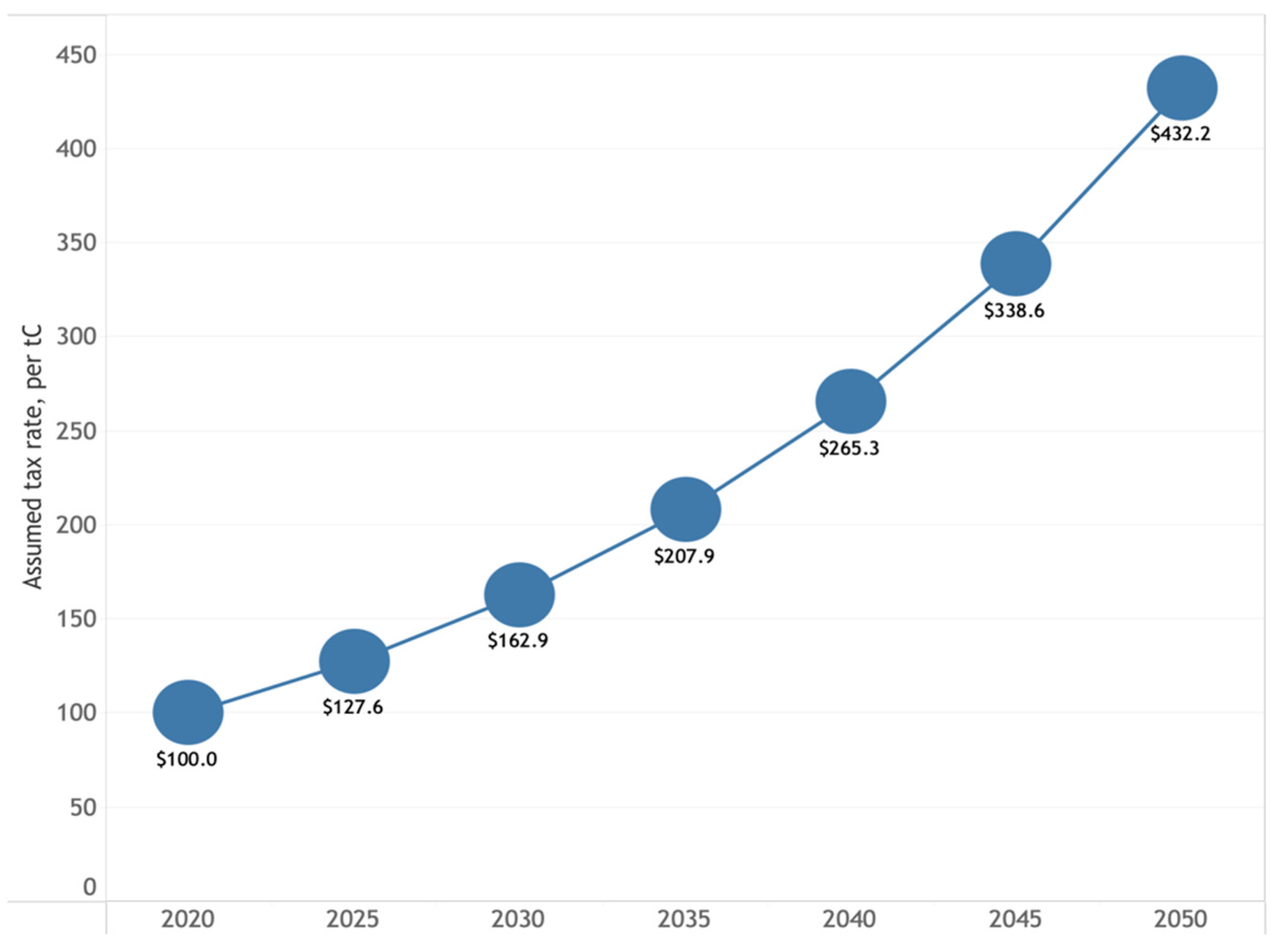
• Emissions tax ($27/tCO₂) and baseline tariffs (Scenario 4);
• Emissions tax ($27/tCO₂) and high tariffs (Scenario 5);
• Emissions tax ($27/tCO₂) and low tariffs (Scenario 6).

Scenario 1 gives the reference scenario, which assumes that the current policies will continue through 2050. Scenarios 2 and 3 allow us to compare how increased/reduced trade friction impacts the global energy trade network. Scenario 4 estimates the impact of a global emissions tax, all else held constant (i.e., climate policy in isolation). Scenarios 5 and 6 estimate the marginal effect of a trade policy when an emissions tax has been imposed, thereby evaluating the interaction of climate policy and trade policy. We will refer to these scenario numbers for the remainder of this paper.

We derive historic tariff rates from a database of product-level ad valorem equivalent rates (AVE) from the World Trade Organization. This database includes AVE at the country–product–year level. These product codes are the same as those used in the BACI database. Tariff data are at the importer–product level, where products are identified by HS6 (Harmonized System, 6 digit) codes. A correspondence table linking HS6 codes to MESSAGEix-represented energy commodities can be found in Table S10 in the Supplementary Materials. We follow methods from Guimbard et al. (2012) and Bouet et al. (2008) to aggregate tariffs while addressing the endogeneity between tariff rates and trade flow; details can also be found in Section 4 in the Supplementary Materials [42,43].

In the baseline scenario, tariffs are held at the historic regional median. In the high tariff scenario, we allow tariff rates to increase to 500% of the historic regional median by 2030, after which it is held constant. This represents an increase that is slightly less than the six-fold increase in tariffs between the U.S. and China in 2019 [44]. In the low tariff scenario, we allow tariff rates to reduce to 0% of the historical median by 2030.

We build the emissions tax scenario by setting the tax to the equivalent of $27/tCO₂ (or $100/tC), increasing by 5% annually. This annual increase has been used in other studies on carbon pricing [45]. Figure 2 displays the emissions tax at each stage of the model horizon.

For each emissions tax scenario, we set tariffs to the historical median (Scenario 4), 500% of the historical median (Scenario 5), or 0% of the historical median (Scenario 6). The emissions tax scenarios and tariff scenarios apply different pressures to global energy trade. Each stage of the energy supply chain has an associated emissions factor; therefore, an emissions tax applies additional pressure throughout the supply chain based on how emissions-intensive each activity is. On the other hand, a tariff scenario impacts only the distribution stage of the energy supply chain. It is a demand-side pressure because it applies an additional cost to the importers of energy. Whether a tariff policy significantly impacts the global energy network would therefore depend on how much this additional cost extends back upstream in the supply chain.

2.4. Energy Security Metrics

Trade portfolio diversity gives a sense of how fungible trade flows are for a given region. When a region imports from a greater number of energy exporters, it is better able to navigate shocks to one of its trade connections because it has options. Alternatively, when an importer relies on a less diverse trade portfolio, it is more vulnerable to changes in its trade partnerships; this is particularly the case when the energy exporter is a region of high political/financial volatility [23]. In this study, we measure trade diversity using the Herfindahl–Hirschman Index (HHI) (see Equation (1)). The HHI measures both the diversity and market concentration of a given portfolio. The index is given by the following formula:

$$HH{I}_{ei}={\displaystyle \sum }_j{s}_{ej}^2$$

(1)

When estimating the HHI of the energy exporter, $s_{ej}^2$ represents the squared share of exports in fuel e going from region i to region j. When estimating the HHI of the energy importer, $s_{ej}^2$ represents the squared share of imports in fuel $e$ going to region $i$ from region $j$. The HHI ranges between approximately 770 and 10,000. (We assume a minimum HHI of around 770 given that there are 13 potential trade partners for each region. If each of these partners receive an equal share of the country’s trade, we would have an HHI equal to 13(7.72), or ~771.) A higher HHI suggests a more concentrated portfolio, whereas a lower HHI suggests a more diverse and balanced portfolio.

3. Results

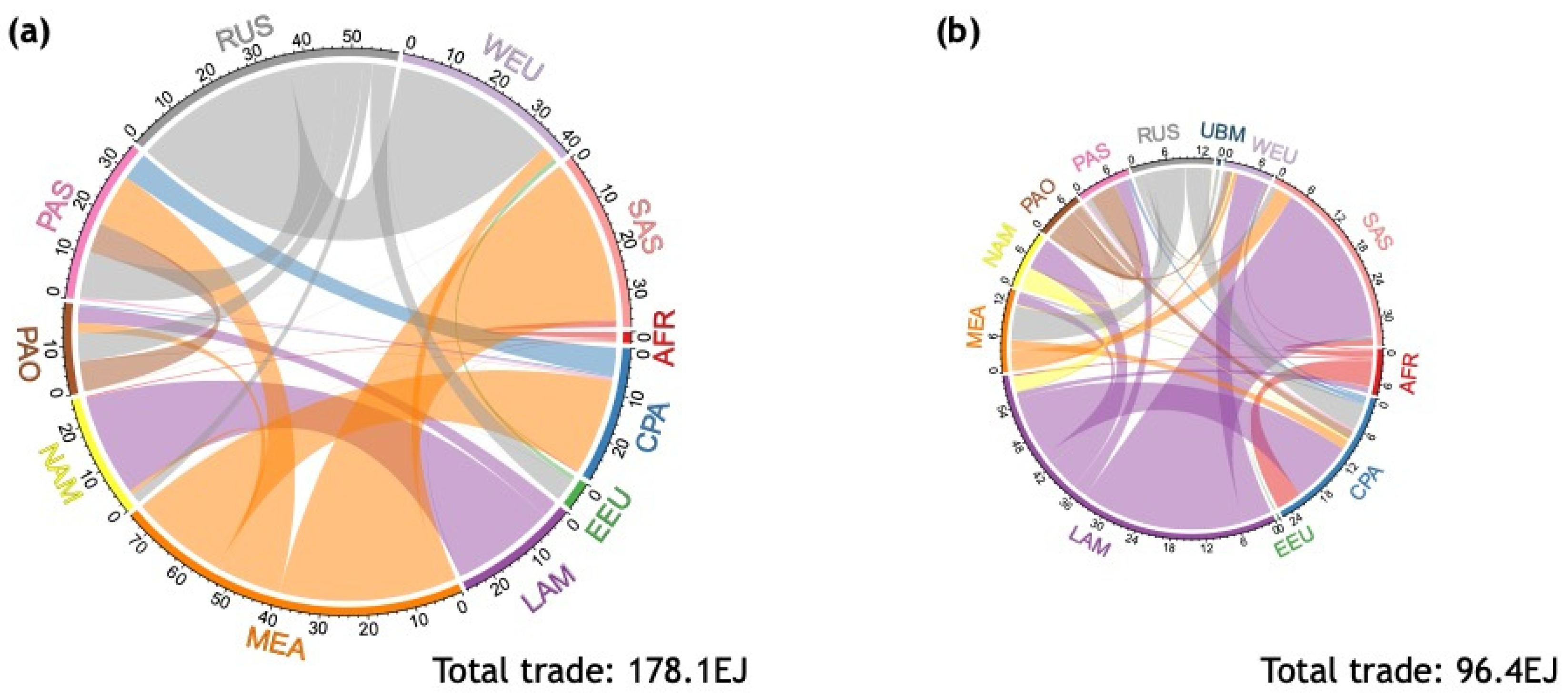
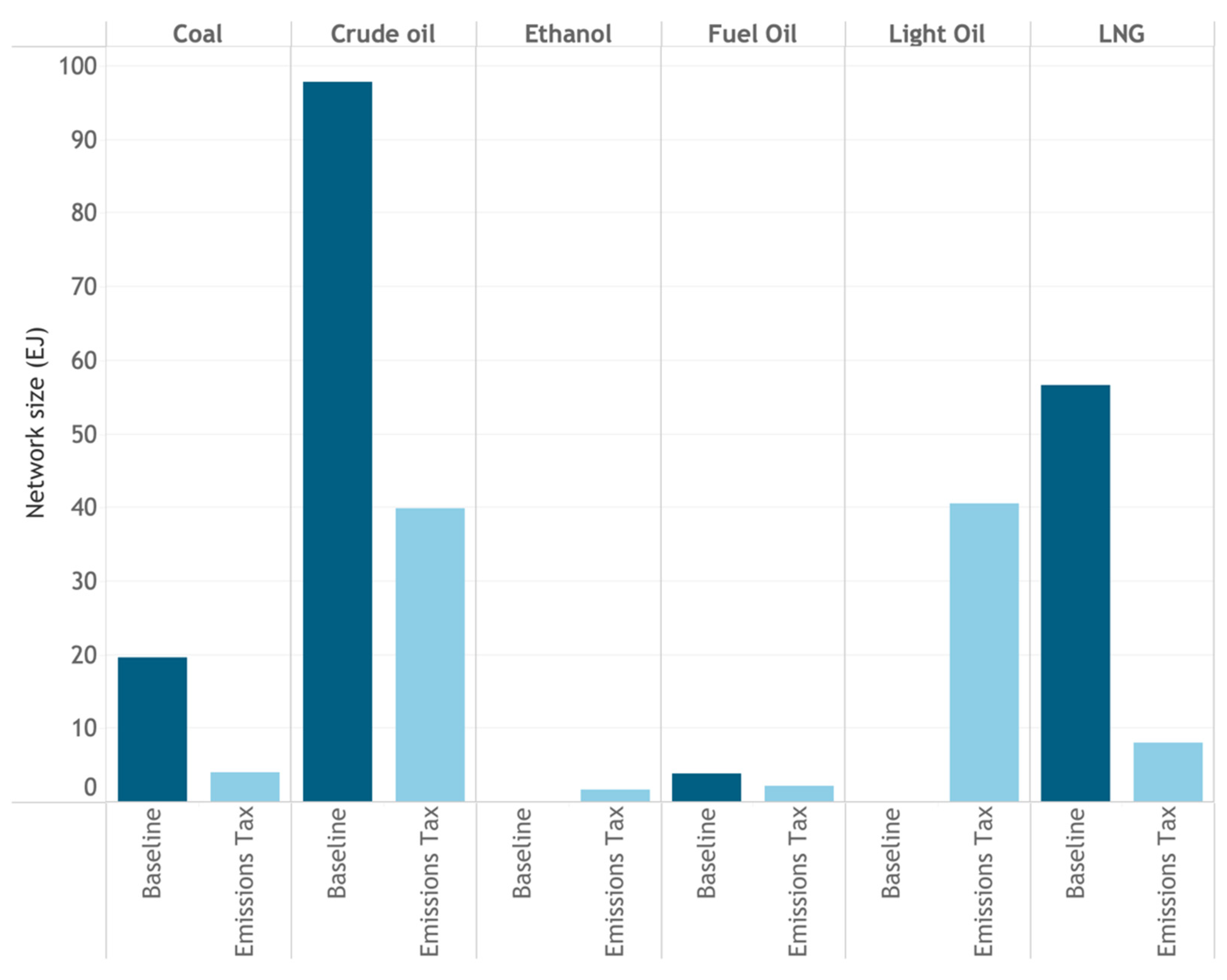
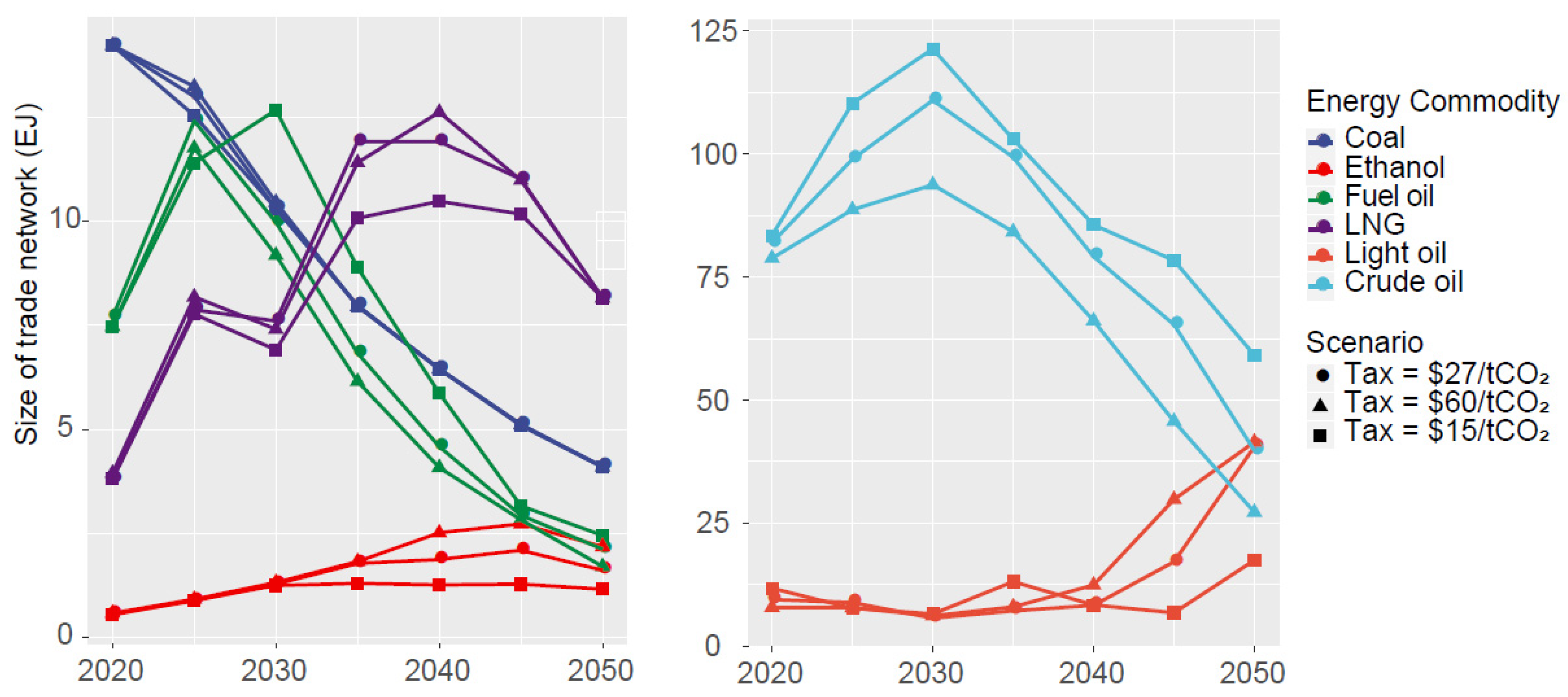
3.1. Effects on Network Size and Composition

Results suggest that tariff policies do not have a significant effect on the composition or size of the global energy trade network. We find that the only effect that the tariff policies have is on global and regional energy system costs. A high tariff scenario increases the total system cost while the low tariff scenario reduces these costs (an ancillary scenario with uniformly increasing tariffs produces similar results, though the magnitude is different).

Conversely, we find that emissions taxes significantly alter the structure and size of the network. Under an emissions tax, the energy network contracts by nearly 50%. The network also becomes more complex; there are more than 72 trade linkages in the emissions tax scenario that were not in the baseline scenario, an increase of roughly 65%. We illustrate this increased complexity through chord diagrams in Figure 3a,b and Figure 4a–h. We have also included a table of all results in Table S11 in the Supplementary Materials.

Figure 3 illustrates the total energy trade network. Each chord is colored by the exporting region and represents the net export flow. In other words, if the Middle East (MEA) exports more LNG to North America (NAM) than it imports from NAM, the difference between the MEA–NAM flow and NAM–MEA flow will be mapped (i.e., only the remaining MEA–NAM flow is illustrated). The network represents the total energy trade network, so the chords represent the sum of exports across energy commodities. Figure 3 suggests that the weight of the global energy trade network shifts from the Middle East to Latin America under an emissions tax. The figure also shows that there is increased complexity under the tax, suggesting that previously dominant flows are spliced into more (and more diverse) linkages. Commodity-specific results presented in Figure 4 support this result and suggest that the driving mechanism for the regional shift in energy exports is driven by a shift in demand from crude oil to light oil.

In other words, a reduction in the amount of crude oil traded under an emissions tax scenario is largely compensated for by an increase in light oil trade (see Figure 5). We discuss the mechanisms underlying the energy-specific results below.

For coal, we observe a stark reduction in the size of the global energy trade network. This is an intuitive result; under an emissions tax, significantly less coal moves through international trade because it becomes more expensive to use (importers are assigned the emissions associated with the trade of each energy commodity). However, in addition to reducing the amount of coal traded, an emissions tax has a secondary effect of making the network far more complex. Under the baseline scenario, there are 10 trade linkages. The linkages are dominated by flows from Centrally Planned Asia and the Pacific OECD (i.e., Australia) to Pacific Asia, and from Russia to Western Europe. Under an emissions tax, there are 33 trade linkages. Except for a large flow from the Pacific OECD to Western Europe, there are no dominating linkages in the network. Of course, the size of the flow here is also relative; the Pacific OECD–Western Europe flow under an emissions tax is 1.05 EJ, while the Pacific OECD–Pacific Asia flow, the largest under the baseline scenario, is 6.57 EJ. We find that this occurs because major coal-producing regions reduce their extraction activities gradually through 2050. This is because the tax rate increases over time. By 2050, there is virtually no coal production across regions and exports are based entirely on stocks from previous years.

The shift away from crude oil is coupled with a dramatic increase in the global light oil trade network. Light oil is a low-density product of crude oil refining or coal liquefication. As an importer, it is more strategic to import light oil over crude oil, even when light oil is simply a secondary product of crude, because the emissions factor is significantly lower. Our results indicate that the under the emissions tax scenario, the Middle East increases its light oil production dramatically using low-yield existing refineries to compensate for the reduction in crude oil demand overseas. This is combined with a dramatic increase in the use of light oil synthesis with carbon capture and sequestration (CCS). On the other hand, Latin America gradually increases its light oil production by increasingly investing in new, higher-yield refineries and CCS. In MESSAGEix, these higher-yield refineries are modeled to have a light oil yield that is 50% greater than that of existing refinery technologies. Over time, Latin America eclipses the Middle East as the dominant light-oil-exporting region.

The size of the LNG trade network contracts significantly under the emissions tax scenario. At the same time, the major exporters shift from Russia and the Middle East to North America and Latin America. Unlike crude oil, which exhibits a marked reduction in trade, LNG simply does not “take off” under an emissions tax scenario. Its import demand, while increasing slightly in the short term, remains relatively low. The demand for ethanol imports increases slightly over time under the emissions tax scenario, while the demand for fuel oil declines.

For all energy commodities, the trade network becomes more complex under an emissions tax scenario. This is largely driven by the direction and magnitude of the policy effect. An emissions tax impacts all parts of the energy supply chain but has a particularly large effect on upstream activities (i.e., production and extraction). This effect moves down the supply chain. A tariff scenario, however, impacts the supply chain at the downstream (i.e., distribution). We find that the policy effect moves down the supply chain more than it moves up. This is best illustrated in the case of the Middle East. In an emissions tax scenario, it becomes prohibitively expensive to extract crude oil in the region because of the high emissions intensity of this upstream activity. This in turn impacts the amount that the Middle East exports, thus influencing the structure of the energy trade network. On the other hand, in the high tariff scenario, the effect of the policy begins with the trade network but does not extend back up to the upstream activity. We find that the extraction of oil in the high tariff scenario (76.2 EJ) is not substantially different from the level of extraction in the baseline (76.7 EJ).

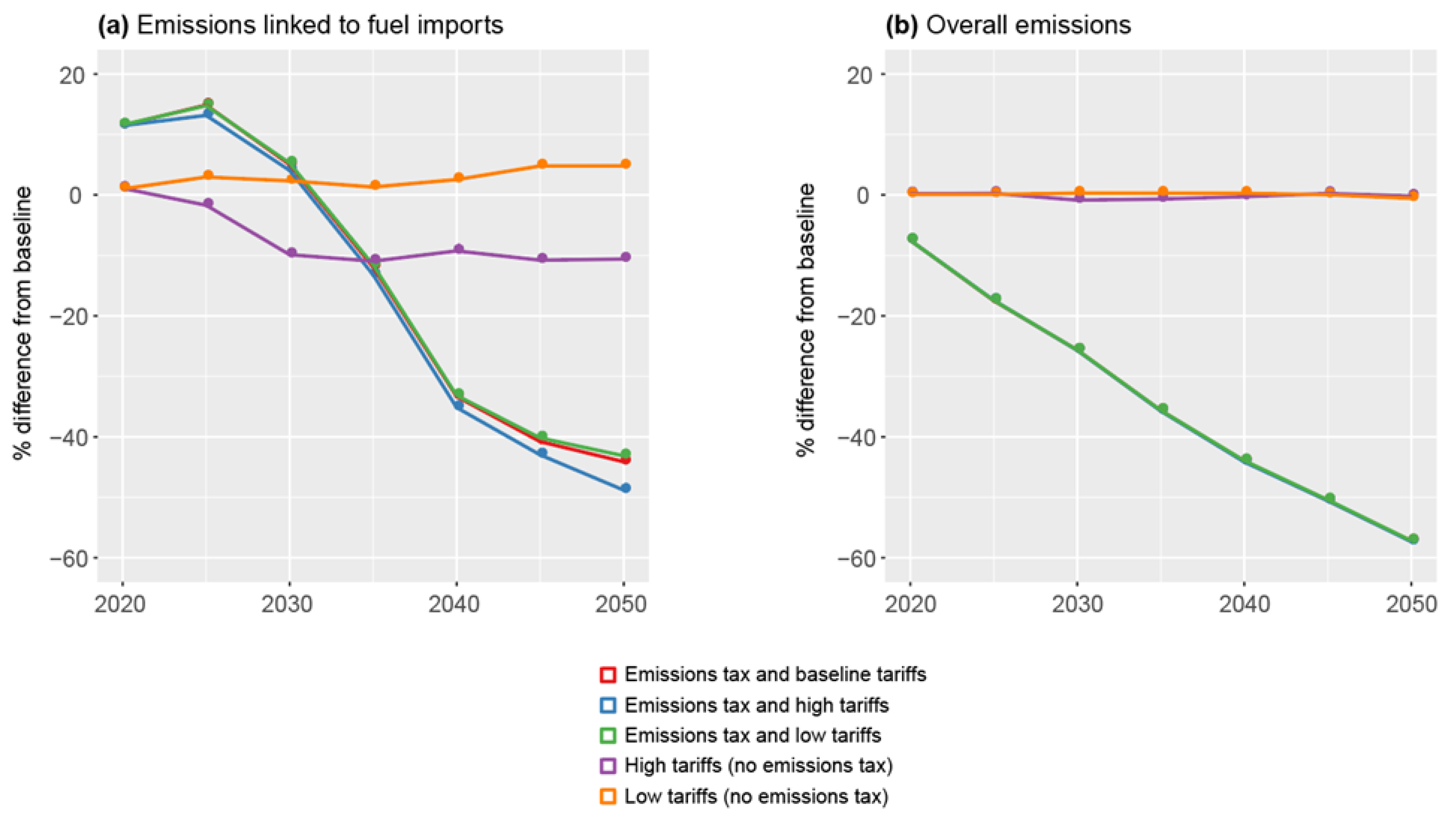
3.2. Effects on Global Emissions

For the purposes of this study, we present emissions in two ways. The first presents emissions associated with energy imports accounted for the importing region [46]. These emissions are based on the amount and emissions factors linked to each energy commodity. In MESSAGEix, when a region exports energy, it is also exporting the emissions related to the trade of these commodities. Therefore, energy exports lead to a reduction in emissions while energy imports lead to an increase in emissions. This allows for a consumption-based accounting of regional emissions. The second presents overall emissions across all energy-related activities. It is important that we present effects on both formats of emissions because a policy that affects trade-related emissions may have minimal (or even opposite) effects on non-trade-related emissions.

Figure 6a presents trajectories of emissions from fuel imports, while Figure 6b presents global emissions trajectories. Emissions from fuel imports are the emissions associated with import activity. Each line is colored by scenario.

Results suggest that sustained, high tariffs can reduce imported emissions by 11.2% in 2050. The low tariff scenario yields a roughly 5% increase in emissions associated with fuel imports. This, however, does not translate to an equivalent effect on overall emissions. We find that the effects of both high and low tariff policies on overall emissions trajectories are minimal. In other words, sustained tariff policies do not lead to lowered emissions and the removal of tariffs does not increase emissions overall. Our results are consistent with the recent literature on the marginal effects of fossil fuel subsidies on global emissions [14].

Unsurprisingly, all emissions tax scenarios result in a large reduction in both imported and overall emissions. Additional trade policies in the presence of an emissions tax have very marginal effects on emissions trajectories. Interestingly, the high tariff scenario (without emissions tax) induces a sizeable reduction in imported emissions. However, because the high tariff scenario only affects trade-related emissions trajectories, this effect does not translate to overall emissions. The tariff only interacts with downstream costs (i.e., trade costs) in energy supply chains. As discussed in Section 3.1, a policy’s effect will be larger if it also impacts the upstream because the effect snowballs as it moves downstream. This is evidenced by the emissions tax, which significantly impacts both upstream and downstream costs. Further, the emissions tax is levied in MESSAGEix based on emissions factors assigned to each activity (e.g., extraction, liquefication, electricity generation). This means that not only is there the production-side effect of increasing extraction and distribution costs, but there is also the demand-side effect of increasing electricity generation costs. A tariff policy’s demand-side effects will only occur when energy is imported (i.e., it will cost more for importers). However, there is no additional cost once the energy has been imported for regions to use it to generate electricity. A global carbon emissions tax, because it more comprehensively impacts the energy supply chain, has a greater impact on emissions reduction, network composition, and the size of the network itself.

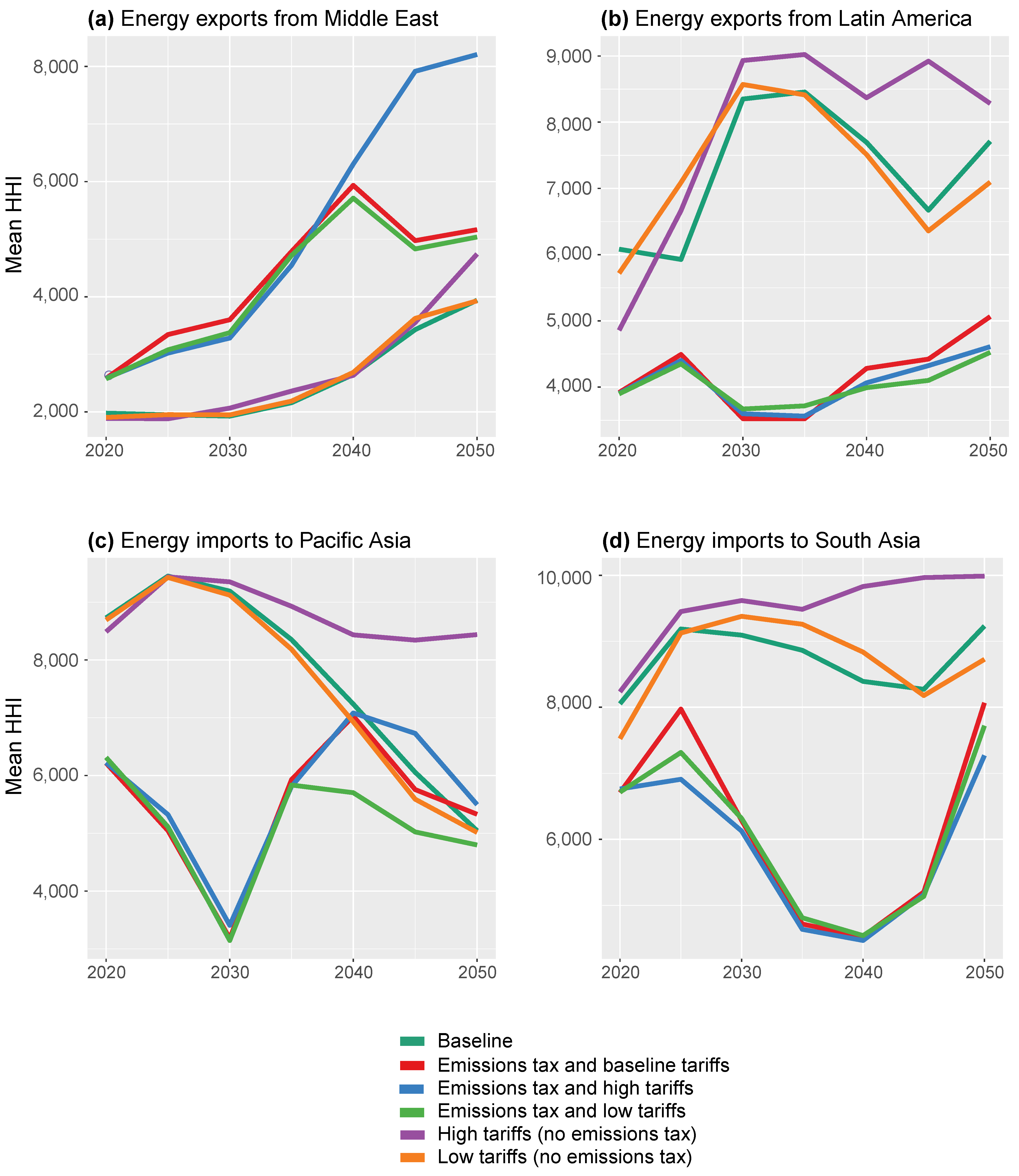
3.3. Effects on Energy Security

We measure energy security using the HHI introduced in the Materials and Methods section of this paper. Figure 7a,b illustrate the trajectories of exporter HHI for the two largest energy exporters (Middle East and Latin America). Figure 7c,d illustrate the trajectories of the importer HHI for the two largest energy importers in the baseline scenario (Pacific Asia and South Asia). Each color represents a different scenario. These results indicate that neither low tariff nor high tariff scenarios influence the general magnitude or direction of both export diversity and import diversity. This is with the exception of the high tariff scenario in Pacific Asia, which exhibits reduced portfolio diversity over time when higher tariffs are levied. In general, the emissions tax scenarios allow regions to maintain a more diverse portfolio of importers. In Pacific Asia and in South Asia, we observe a dramatic decrease in HHI (i.e., higher portfolio diversity) in the short term. For Pacific Asia, this reflects a shift away from crude oil and toward light oil from Latin America and Oceania. For South Asia, this reflects a shift away from LNG from the Middle East and toward light oil from these same regions. In other words, dependence on one commodity is split into two or more commodities from two or more regions. This is consistent with the effects of the emissions tax on the global fuel trade network, as increased complexity in the network is facilitated when each region has more trade linkages and balances its imports and/or exports among these linkages. Interestingly this effect does not translate generally to energy exporters; while the emissions tax allows for increased diversity in energy exports from Latin America, it reduces diversity in energy exports from Middle East. This is in fact a function of the dramatic reduction in crude oil demand from importing regions under the emissions tax scenario.

Our results suggest that an emissions tax can induce increased complexity in the trade network, which subsequently leads to increased portfolio security. However, it is important to note here that there are also factors driving baseline trends. This study assumes Shared Socioeconomic Pathway 2 (SSP2) as the basis for the future population and GDP growth. The SSPs represent a set of internally consistent socioeconomic assumptions based on different narratives for the world’s future, including the world’s population and economic growth [47]. SSP2 is the “middle-of-the-road” pathway that includes (for example) relatively high population and GDP growth in India [48]. We see this reflected in the energy security trajectories of this study. Figure 7 shows that, in the baseline scenario, South Asia (including India) presents increased import diversity. On the other hand, the Middle East shows a decrease in export diversity. This is driven by crude and light oil. As the oil demand in South Asia increases (driven by GDP and population growth in India), it demands imports from more regions. These regions shift their oil exports to South Asia and reduce their exports to other regions. In some cases, the original trade flow to a non-South Asia importer was small to begin with, so the trade flow reduces to zero. This reduces the energy exporters’ trade diversity and increases the dependence on sustained demand from India. Over time, Latin America becomes the dominant exporter of light oil. By 2050, light oil eclipses crude oil in the global energy market. Because India increases its reliance on Latin America, we observe an increase in the HHI toward 2050, which is indicative of a more concentrated import portfolio. This trajectory is not the result of any one policy, but rather the consequence of underlying socioeconomic pathways. This has implications for energy export security in the future, even without any additional policy effects. This exercise underscores the importance of including underlying socioeconomic assumptions in energy policy evaluations.

3.4. Sensitivity Analysis

We conduct two main sensitivity analyses on our results to check their robustness. The first is with regard to the tax rate in our emissions tax scenario. All scenarios assume a starting tax of $27/tCO₂ in 2020, increasing by 5% annually thereafter. We also test a “low emissions tax” scenario with a starting rate at $15/tCO₂ and a “high emissions tax” scenario with a starting rate of $60/tCO₂. We apply the 5% annual increase in both cases. By changing the tax rate, we are testing whether the existence of a tax or the underlying tax rate influences our results. In other words, if the $15/tCO₂ scenario produces results that are very similar to those of the $27/tCO₂ scenario, it is the existence of the tax and not the tax rate that catalyzes the dramatic changes to the global energy trade network that we present.

This result of this sensitivity analysis, in Figure 8, indicates that our findings are robust to changing tax rates, except in the case of crude oil and light oil. This is indicative of the tradeoff between the two commodities. Under the high tax scenario, crude oil trade constrains (from 39.8 EJ to 27.2 EJ) whereas light oil trade increases (40.5 EJ to 41.5 EJ). Under the low tax scenario, crude oil trade increases (to 59.1 EJ) while light oil trade constrains (to 17.5 EJ). This means that certain commodities are more sensitive to the emissions tax than others and that crude oil is particularly sensitive. This is consistent with the rationale presented in Section 3.1, in which we propose that the emissions tax affects costs throughout the energy supply chain and so commodities that have particularly emissions-intensive upstream costs will be disproportionately impacted by a tax. In addition to sliding the tax rate, we conduct a sensitivity analysis based on emissions factors. As in the first sensitivity analysis, the purpose of this analysis is to test whether the mechanism proposed in Section 3.1 holds under varying levels within each scenario.

In this case, we test whether the Middle East is so heavily impacted because crude oil extraction is a very emissions-intensive activity. (While the emissions factor for oil extraction in the Middle East is not higher than that of other regions, most crude oil reserves are located in the Middle East. Because most extraction takes place there, changes in the emissions factor would impact it most.) Our null hypothesis is that if the Middle East were to reduce its emissions factor of crude oil extraction by 50%, the global energy network under an emissions tax would more closely resemble that of the baseline scenario without the tax. In other words, the null hypothesis states that the upstream emissions factor in the Middle East is what drives the dramatic effects of the emissions tax. To run this analysis, we run the emissions tax scenarios (at $27/tCO₂) while setting extraction technologies in MESSAGEix to 50% of their baseline levels.

Our results suggest that while lowering the emissions factors of crude oil extraction in the Middle East has a slight effect on the composition of the global energy trade network, the presence of the emissions tax still causes dramatic changes compared to the baseline. This means that lowering the emissions factor of the Middle East’s crude oil extraction is a significant, but not total, explanatory factor in determining the shape of the energy trade network. This result is consistent with the mechanism described in Section 3.1; the emissions tax has a dramatic effect on the trade network because it hits all levels of the energy supply chain. This result is also consistent with the first sensitivity analysis on tax levels.

4. Discussion

4.1. Limitations of This Study

The main limitations of this study stem from underlying assumptions for policy scenarios. The first assumption that we make is that tariff rates are increased and reduced concurrently across all regions. In reality, one region may increase a tariff, which leads another to rise their tariff rates, and so on. In addition, if a region has low tariffs historically, it will also have relatively low tariffs even after being multiplied by a factor of five in our high tariff scenario. We also run an ancillary scenario in which tariffs increase uniformly across regions, but do not include it in our main list of scenarios for simplicity. The same holds for a global emissions tax; perhaps one region applies a tax first, which affects another region’s decision to impose a tax. Here, we assume a global carbon emission tax. Thus, we do not capture any temporal or spatial heterogeneity in this scenario setup for the application of policies in this regard.

We also assume in our underlying country-level data that all trade between countries is shipped by sea, along the shortest shipping routes. This affects our calculation of the marginal effect of distance on trade costs. We believe that this assumption is not unrealistic, however. Firstly, 90% of total trade is conducted along maritime routes [49]. Secondly, because of shipping costs (e.g., fuel costs, insurance), most shipping companies will aim to take the shortest route to transport commodities.

One limitation of the MESSAGEix global energy model is its spatial aggregation. Currently, the world is represented through 14 regions. However, there are country-level (and even sub-national-level) trends that influence the structure of global energy markets. We are not able to capture this heterogeneity in this study. Furthermore, some regions combine countries that have very different energy systems; for instance, the Pacific OECD includes Japan (a major energy importer) and Australia (a major energy exporter). Note, however, that MESSAGEix includes constraints to restrict Japan from tapping into the abundant energy resources available in Australia. In other words, the model setup ensures that the Japanese and Australian energy systems operate separately at the sub-regional level.

4.2. Trade Frictions Make Climate Policy More Expensive

The emissions tax scenarios systematically shifted the composition and size of the global energy trade network. It added more linkages among more regions, illustrating that this type of ambitious climate policy requires more interactions among trading regions. At the same time, this type of policy may be exceedingly difficult to implement given the current political landscape. It is therefore important to understand the implications of passing such a policy under different political circumstances. Let us say that we use a tariff policy as a proxy for trade “friendliness” and sustained high tariffs lead to an unfriendly trade environment. Under an emissions tax, the trade network will alter regardless of the friendliness of the trade environment; however, the cost of global and regional energy systems may increase. Our hypothesis is that if an ambitious climate policy is undertaken, the optimal (in this case, cost-minimizing) way to prepare the trade network for such drastic shifts is to remove frictions to trade.

We validate this argument by illustrating the difference in regional energy system costs (compared to the baseline) when tariff policies are applied or removed after a carbon emissions tax is applied. We illustrate these marginal differences for major energy-exporting regions (Latin America, Middle East, and Russia), major energy-importing regions (Pacific Asia, South Asia, and Centrally Planned Asia), and across all regions.

Figure 9 suggests that when a sustained tariff policy is applied (i.e., the trade environment is less friendly), the regional energy system costs for importing regions go up dramatically. For energy-exporting regions, the energy system costs go down initially but increase in 2050. Overall, the average system cost increases across all regions. Conversely, when energy tariffs are removed, regional energy system costs generally decline, with the exception of energy-exporting regions, which exhibit a slight increase in costs. Ultimately, the effect of additional energy tariff policies in the presence of an emissions tax is much larger for energy-importing regions than they are for energy-exporting regions. This is because energy tariffs are applied to the importer. However, the effects to importers are large enough that they dictate the direction of average regional energy system costs. Emissions taxes will apply a large cost to the global energy system if trade frictions are not removed.

4.3. Energy Security Is Supply Chain Security, and Vice Versa

The Russian invasion of Ukraine in February 2022, beyond swiftly becoming a humanitarian crisis, upended global energy markets. The impacts have been particularly pronounced in the EU. In addition to compromising global energy security, this major energy shock will have long-lasting impacts on the supply chains that underpin the global economy [50]. These supply chains produce energy technologies that are needed to accelerate the clean energy transition and realize global climate goals. In other words, energy security risks compromise supply chain security, and supply chain security risks compromise energy security. This type of interplay underscores the need to integrate complex trade networks in IAM work.

The results of the high tariff scenario can act as a proxy for a scenario with high trade friction, i.e., what we are seeing now with Russia. The U.S., the EU, and Japan have sanctioned Russian energy as the war continues. This sanction increases the cost of trade. However, the increase is only on a specific, high-emissions-intensity commodity. What this means is that the bilateral schema in MESSAGEix can be used to identify whether the clean energy transition could happen faster and cheaper than past scenarios have anticipated due to changes in Russian trade linkages. This is an important area for future research.

5. Conclusions

Globalization is inextricably tied to energy transitions; regional energy systems are made up not only of domestic flows but also the ways in which the region interacts with others. The robust trade network that is formed by these interactions has not been explicitly modeled in widely used global energy models. This study provides a development to the MESSAGEix model by modeling the trade of energy commodities bilaterally and tracing the flows of these commodities explicitly from the exporting region to the importing region. This bilateral representation allows us to closely examine the effects of trade policies on emissions, as well as the effects of climate policies on trade network structures. It also allows us to explore the implications of these policies on regional energy security.

Our results indicate that tariff policies, taken independently, do not significantly impact the structure of the fuel trade network. Sustained high tariffs do significantly reduce emissions that are associated with fuel imports, but do not change the trajectory of overall emissions compared to the baseline. This is also consistent with a recent study, which found that imported fuel is substituted by other domestic fossil-fuel-based solutions [17]. An emissions tax of $27/tCO₂ dramatically alters the fuel trade network in terms of both size (reducing it by nearly 50%) and the composition of fuels. The emissions tax scenario induces large reductions in global emissions; however, these reductions are not driven by changes in trade-related emissions, but rather occur from systemic reductions throughout the energy supply chain.

Importantly, a carbon emission tax increases the complexity of the trade network by forming more trade linkages compared to the baseline. This increases the energy security of energy importers and most energy exporters, with the exception of the Middle East, which relies heavily on the export of crude oil (demand for which is dramatically reduced under an emissions tax). The increased diversity of trade portfolios underscores the need for international cooperation to optimally effect a global emissions tax. This may be difficult to achieve given the current political landscape, but it is important to understand the implications of such climate policies under different political circumstances. A fully cooperative tariff policy can be used as a proxy for “friendliness” in energy trade, while sustained high tariffs lead to an unfriendly trade environment. Under an emissions tax, the trade network will alter regardless of the friendliness of the trade environment. However, the cost of global and regional energy systems will increase, which affects the efforts of these regions in achieving their climate targets. If an ambitious climate policy is undertaken, the optimal, cost-effective way to prepare the trade network for such drastic shifts is to remove frictions to trade, such as bans and sanctions.

This study provides an entryway into understanding the interactions between climate and trade policy in the context of energy security and emissions. Furthermore, it underscores the importance of including an explicit representation of trade networks in global energy models. Future research on this topic should investigate the additional trade feedback stemming from existing and imminent climate change impacts to geopolitics in energy-exporting regions. Another direction of future research may further explore the uncertainty of energy trajectories under climate and trade policy scenarios, particularly with regard to future demand for fossil fuels. Finally, the objective function in MESSAGE is to minimize global energy system costs; however, one can imagine that there are multiple objectives in resolving energy demands, including sustainability. We anticipate that a multi-objective optimization framework could be applied to the same questions presented in this paper.

References

1. Riahi, K.; Bertram, C.; Huppmann, D.; Rogelj, J.; Bosetti, V.; Cabardos, A.-M.; Deppermann, A.; Drouet, L.; Frank, S.; Fricko, O.; et al. Cost and Attainability of Meeting Stringent Climate Targets without Overshoot. Nat. Clim. Chang. 2021, 11, 1063–1069. [Google Scholar] [CrossRef]
2. Rogelj, J.; den Elzen, M.; Höhne, N.; Fransen, T.; Fekete, H.; Winkler, H.; Schaeffer, R.; Sha, F.; Riahi, K.; Meinshausen, M. Paris Agreement Climate Proposals Need a Boost to Keep Warming Well below 2 °C. Nature 2016, 534, 631–639. [Google Scholar] [CrossRef] [PubMed]
3. UNFCCC. INDCs as Comunicated by Parties; UNFCCC: Paris, France, 2015. [Google Scholar]
4. Dong, C.; Dong, X.; Jiang, Q.; Dong, K.; Liu, G. What Is the Probability of Achieving the Carbon Dioxide Emission Targets of the Paris Agreement? Evidence from the Top Ten Emitters. Sci. Total Environ. 2018, 622–623, 1294–1303. [Google Scholar] [CrossRef] [PubMed]
5. Pischke, E.C.; Solomon, B.; Wellstead, A.; Acevedo, A.; Eastmond, A.; De Oliveira, F.; Coelho, S.; Lucon, O. From Kyoto to Paris: Measuring Renewable Energy Policy Regimes in Argentina, Brazil, Canada, Mexico and the United States. Energy Res. Soc. Sci. 2019, 50, 82–91. [Google Scholar] [CrossRef]
6. Cai, H.; Huang, S.; Wu, Z. The Impact of COVID-19 on the International Energy Trade Network Centrality and Community Structures. Appl. Econ. Lett. 2022. [Google Scholar] [CrossRef]
7. Hao, X.; An, H.; Qi, H.; Gao, X. Evolution of the Exergy Flow Network Embodied in the Global Fossil Energy Trade: Based on Complex Network. Appl. Energy 2016, 162, 1515–1522. [Google Scholar] [CrossRef]
8. Zhong, W.; An, H.; Shen, L.; Fang, W.; Gao, X.; Dong, D. The Roles of Countries in the International Fossil Fuel Trade: An Emergy and Network Analysis. Energy Policy 2017, 100, 365–376. [Google Scholar] [CrossRef]
9. Amaro, S. Russia Nears Gas Shutdown in Europe as Germany Rejects Claims It Can’t Fulfill Contracts. Available online: https://www.cnbc.com/2022/07/19/russia-nears-gas-shutdown-in-europe-as-germany-rejects-claims-it-cant-fulfil-contracts.html (accessed on 11 August 2022).
10. Natural Gas Supply Statistics. Available online: https://ec.europa.eu/eurostat/statistics-explained/index.php?title=Natural_gas_supply_statistics (accessed on 11 August 2022).
11. From Deep Crisis, Profound Change. Available online: https://rmi.org/insight/from-deep-crisis-profound-change/ (accessed on 11 August 2022).
12. China’s Spending on Russian Oil, Gas, Coal Jumps to $6.4 Billion in June—Bloomberg. Available online: https://www.bloomberg.com/news/articles/2022-07-20/china-s-spending-on-russian-energy-jumps-to-6-4-billion-in-june (accessed on 11 August 2022).
13. Jakob, M. Climate Policy and International Trade—A Critical Appraisal of the Literature. Energy Policy 2021, 156, 112399. [Google Scholar] [CrossRef]
14. Jewell, J.; McCollum, D.; Emmerling, J.; Bertram, C.; Gernaat, D.E.H.J.; Krey, V.; Paroussos, L.; Berger, L.; Fragkiadakis, K.; Keppo, I.; et al. Limited Emission Reductions from Fuel Subsidy Removal except in Energy-Exporting Regions. Nature 2018, 554, 229–233. [Google Scholar] [CrossRef]
15. Jewell, J.; Vinichenko, V.; McCollum, D.; Bauer, N.; Riahi, K.; Aboumahboub, T.; Fricko, O.; Harmsen, M.; Kober, T.; Krey, V.; et al. Comparison and Interactions between the Long-Term Pursuit of Energy Independence and Climate Policies. Nat. Energy 2016, 1, 16073. [Google Scholar] [CrossRef] [Green Version]
16. Matsuoka, Y.; Kainuma, M.; Morita, T. Scenario Analysis of Global Warming Using the Asian Pacific Integrated Model (AIM). Energy Policy 1995, 23, 357–371. [Google Scholar] [CrossRef]
17. Huppmann, D.; Gidden, M.; Fricko, O.; Kolp, P.; Orthofer, C.; Pimmer, M.; Kushin, N.; Vinca, A.; Mastrucci, A.; Riahi, K.; et al. The MESSAGE Integrated Assessment Model and the Ix Modeling Platform (Ixmp): An Open Framework for Integrated and Cross-Cutting Analysis of Energy, Climate, the Environment, and Sustainable Development. Environ. Model. Softw. 2019, 112, 143–156. [Google Scholar] [CrossRef]
18. Stehfest, E.; voor de Leefomgeving, P. Integrated Assessment of Global Environmental Change with IMAGE 3.0: Model Description and Policy Applications; PBL Netherlands Environmental Assessment Agency: The Hague, NL, 2014; ISBN 978-94-91506-71-0. [Google Scholar]
19. Hare, B.; Brecha, R.; Schaeffer, M. Integrated Assessment Models: What Are They and How Do They Arrive at Their Conclusions? Climate Analytics: Berlin, DE, USA, 2018. [Google Scholar]
20. Berdysheva, S.; Ikonnikova, S. The Energy Transition and Shifts in Fossil Fuel Use: The Study of International Energy Trade and Energy Security Dynamics. Energies 2021, 14, 5396. [Google Scholar] [CrossRef]
21. Yergin, D. Ensuring Energy Security. Foreign Affairs 2006, 85, 69–82. [Google Scholar] [CrossRef]
22. Greene, D.L. Measuring Energy Security: Can the United States Achieve Oil Independence? Energy Policy 2010, 38, 1614–1621. [Google Scholar] [CrossRef]
23. Le Coq, C.; Paltseva, E. Measuring the Security of External Energy Supply in the European Union. Energy Policy 2009, 37, 4474–4481. [Google Scholar] [CrossRef]
24. Kruyt, B.; van Vuuren, D.P.; de Vries, H.J.M.; Groenenberg, H. Indicators for Energy Security. Energy Policy 2009, 37, 2166–2181. [Google Scholar] [CrossRef]
25. International Trade during the COVID-19 Pandemic: Big Shifts and Uncertainty. Available online: https://www.oecd.org/coronavirus/policy-responses/international-trade-during-the-covid-19-pandemic-big-shifts-and-uncertainty-d1131663/ (accessed on 19 July 2022).
26. Tollefson, J. What the War in Ukraine Means for Energy, Climate and Food. Nature 2022, 604, 232–233. [Google Scholar] [CrossRef] [PubMed]
27. Gao, C.; Sun, M.; Shen, B. Features and Evolution of International Fossil Energy Trade Relationships: A Weighted Multilayer Network Analysis. Appl. Energy 2015, 156, 542–554. [Google Scholar] [CrossRef]
28. Chen, G.Q.; Wu, X.F. Energy Overview for Globalized World Economy: Source, Supply Chain and Sink. Renew. Sustain. Energy Rev. 2017, 69, 735–749. [Google Scholar] [CrossRef]
29. Shepard, J.U.; Pratson, L.F. Hybrid Input-Output Analysis of Embodied Energy Security. Appl. Energy 2020, 279, 115806. [Google Scholar] [CrossRef]
30. Schrattenholzer, L. The Energy Supply Model Message; Research Reports/Internationales Institut für Angewandte Systemanalyse; International Institut for Applied Systems Analysis: Laxenburg, Austria, 1981; ISBN 978-3-7045-0024-3. [Google Scholar]
31. Elliott, J.; Foster, I.; Kortum, S.; Munson, T.; Cervantes, F.P.; Weisbach, D. Trade and Carbon Taxes. Am. Econ. Rev. 2010, 100, 465–469. [Google Scholar] [CrossRef]
32. Bergman, L. General Equilibrium Effects of Environmental Policy: A CGE-Modeling Approach. Environ. Resour. Econ. 1991, 1, 43–61. [Google Scholar] [CrossRef]
33. Rivers, N.; Schaufele, B. The Effect of Carbon Taxes on Agricultural Trade: Effect of Carbon Taxes on Agricultural Trade. Can. J. Agric. Econ./Rev. Can. D’agroeconom. 2015, 63, 235–257. [Google Scholar] [CrossRef]
34. Martin, R.; de Preux, L.B.; Wagner, U.J. The Impact of a Carbon Tax on Manufacturing: Evidence from Microdata. J. Public Econ. 2014, 117, 1–14. [Google Scholar] [CrossRef]
35. Messner, S.; Schrattenholzer, L. MESSAGE–MACRO: Linking an Energy Supply Model with a Macroeconomic Module and Solving It Iteratively. Energy 2000, 25, 267–282. [Google Scholar] [CrossRef]
36. UNFCCC. Climate Change 2014: Mitigation of Climate Change: Working Group III Contribution to the Fifth Assessment Report of the Intergovernmental Panel on Climate Change; Intergovernmental Panel on Climate Change; Edenhofer, O., Ed.; Cambridge University Press: New York, NY, USA, 2014; ISBN 978-1-107-05821-7. [Google Scholar]
37. Sullivan, P.; Krey, V.; Riahi, K. Impacts of Considering Electric Sector Variability and Reliability in the MESSAGE Model. Energy Strategy Rev. 2013, 1, 157–163. [Google Scholar] [CrossRef]
38. Zhang, S.; Yi, B.-W.; Worrell, E.; Wagner, F.; Crijns-Graus, W.; Purohit, P.; Wada, Y.; Varis, O. Integrated Assessment of Resource-Energy-Environment Nexus in China’s Iron and Steel Industry. J. Clean. Prod. 2019, 232, 235–249. [Google Scholar] [CrossRef]
39. Zhao, F.; Fan, Y.; Zhang, S. Assessment of Efficiency Improvement and Emission Mitigation Potentials in China’s Petroleum Refining Industry. J. Clean. Prod. 2021, 280, 124482. [Google Scholar] [CrossRef]
40. Gaulier, G.; Zignago, S. BACI: A World Database of International Trade at the Product-Level 1995–2004; Centre D’Etudes Prospectives et D’Informations Internationales (CEPII): Paris, France, 2010. [Google Scholar]
41. Helpman, E.; Melitz, M.; Rubinstein, Y. Estimating Trade Flows: Trading Partners and Trading Volumes. Q. J. Econ. 2008, 123, 441–487. [Google Scholar] [CrossRef] [Green Version]
42. Guimbard, H.; Jean, S.; Mimouni, M.; Pichot, X. MAcMap-HS6 2007, an Exhaustive and Consistent Measure of Applied Protection in 2007. Économie Int. 2012, 130, 99–121. [Google Scholar] [CrossRef]
43. Bouët, A.; Decreux, Y.; Fontagné, L.; Jean, S.; Laborde, D. Assessing Applied Protection across the World. Rev. Int. Econ. 2008, 16, 850–863. [Google Scholar] [CrossRef]
44. York, E. Tracking the Economic Impact of Tariffs. Tax Foundation, 1 April 2022. [Google Scholar]
45. Barron, A.R.; Hafstead, M.A.C.; Morris, A.C. Policy Insights from Comparing Carbon Pricing Modeling Scenarios; Brookings Institution: Washington, DC, USA, 2019. [Google Scholar]
46. Jakob, M.; Ward, H.; Steckel, J.C. Sharing Responsibility for Trade-Related Emissions Based on Economic Benefits. Glob. Environ. Chang. 2021, 66, 102207. [Google Scholar] [CrossRef]
47. Riahi, K.; van Vuuren, D.P.; Kriegler, E.; Edmonds, J.; O’Neill, B.C.; Fujimori, S.; Bauer, N.; Calvin, K.; Dellink, R.; Fricko, O.; et al. The Shared Socioeconomic Pathways and Their Energy, Land Use, and Greenhouse Gas Emissions Implications: An Overview. Glob. Environ. Chang. 2017, 42, 153–168. [Google Scholar] [CrossRef]
48. Fricko, O.; Havlik, P.; Rogelj, J.; Klimont, Z.; Gusti, M.; Johnson, N.; Kolp, P.; Strubegger, M.; Valin, H.; Amann, M.; et al. The Marker Quantification of the Shared Socioeconomic Pathway 2: A Middle-of-the-Road Scenario for the 21st Century. Glob. Environ. Chang. 2017, 42, 251–267. [Google Scholar] [CrossRef]
49. Rodrigue, J.-P.; Comtois, C.; Slack, B. The Geography of Transport Systems, 4th ed.; Routledge: London, UK, 2016; ISBN 978-1-315-61815-9. [Google Scholar]
50. Shepard, J.U.; Pratson, L.F. The Myth of US Energy Independence. Nat. Energy 2022, 7, 462–464. [Google Scholar] [CrossRef]
Figure 1. Schematics of the MESSAGEix global energy model. (a) Illustration of the “global pool schema” representation of international trade. There are 14 representative regions. Each region can export to (green) or import from (red) a global pool of each energy commodity (e.g., crude oil). (b) Energy flow in the global schema through inputs and output. Model “levels” are in green (e.g., primary, secondary, export, final), nodes are in blue (i.e., regions), commodities are in yellow (e.g., coal, crude oil), technologies are in orange (e.g., exports, imports), and parameters are in black (e.g., input, output). AFR represents Africa, GLB represents the global node, and WEU represents Western Europe. This flow therefore represents crude oil exports from Africa to Western Europe. (c) Illustration of the “bilateral trade schema” for international trade. We explicitly model bilateral trade flows for each energy commodity, thus representing trade as a network rather than a pooled resource. (d) Flow of energy in bilateral representation of trade. Note here that technologies now explicitly define the destination of, in this instance, crude oil exports. Commodities also explicitly denote the destination (“crudeoil_weu”).
Energies 15 06171 g001
Figure 2. Emissions tax rates, set globally, by model year. We allow the tax to start at $100/tC and increase by 5% annually.
Energies 15 06171 g002
Figure 3. The energy trade network in 2050 under the baseline scenario (a) and under an emissions tax scenario (b). This figure illustrates the network across energy commodities, (i.e., it is the sum of coal, crude oil, ethanol, fuel oil, light oil, LNG, methanol, and liquid hydrogen). Each chord represents the net export flow. The units of these chord diagrams are in EJ. Regions are represented as follows: AFR = Africa, CPA = Centrally Planned Asia, EEU = Eastern Europe, LAM = Latin America, MEA = Middle East and North Africa, NAM = North America, PAO = Pacific OECD, PAS = Pacific Asia, RUS = Russia, SAS = South Asia, WEU = Western Europe. The color of the traded volume is identical to the exporter region.
Energies 15 06171 g003
Figure 4. Trade networks in 2050 under the baseline scenario (left column) and emissions tax scenario (right column). (a,b) represent coal trade, (c,d) represent crude oil trade, (e,f) represent light oil trade, (g,h) represent LNG trade. Total trade for the given energy commodity is given in the corresponding box in EJ.
Energies 15 06171 g004
Figure 5. Total global trade size by energy commodity in 2050 in baseline and emissions tax scenarios.
Energies 15 06171 g005
Figure 6. Changes from the baseline scenario for the global level. The figure is in terms of emissions associated with fuel imports (a) and overall (b). Each line is colored by a different scenario.
Energies 15 06171 g006
Figure 7. Energy security based on mean Herfindahl–Hirschman Index (HHI) values for major importers and exporters (the lower the index, the higher energy security and diversity). The figure presents the top two energy-exporting regions (a,b) and top two energy-importing regions (c,d). Lines are colored by scenario.
Energies 15 06171 g007
Figure 8. Sensitivity analysis with varying emissions tax levels. Colors represent energy commodities; shapes represent the various emissions tax scenarios. We present crude oil and light oil in a separate figure as these two commodities are traded at a much larger scale than the other commodities.
Energies 15 06171 g008
Figure 9. Average regional energy system costs (2020–2050). Major exporting regions include Latin America, the Middle East, and Russia. Major importing regions include Pacific Asia, South Asia, and Centrally Planned Asia. All regions include these regions and the remaining 8 regions represented in MESSAGE. Blue lines represent regional costs under an emissions tax and high tariffs, while red lines represent regional costs under an emissions tax and reduced/no tariffs.
Energies 15 06171 g009