Mathematical Model of Shale Oil Seepage at Micro-Nano Pore Scale

Abstract

Due to the unclear seepage mechanism for shale oil, it is hard to establish a reasonable mathematical model to describe the flowing law. In this study, a real shale pore structure was reconstructed with CT scanning and a numerical model of fluid flowing in the real shale pore is developed with COMSOL, based on the boundary slip at the micro-nano pore scale to study the causes of nonlinear seepage. A two-fluid model is employed to establish a simple mathematical model to describe the relationship between the flow rate and the pressure gradient using the effective slip length to account for the influence of pore structure and true slip, and the established model is verified with experimental data coming from Jiyang shale oil. The results indicated that the pore structure greatly affected the shape of the seepage curve. With the increase in displacement pressure, the percentage of fluid involved in the flow increased until it became stable, showing a changing trend from nonlinearity to linearity. The established model can fit the experimental data well and reasonably characterize the nonlinear seepage of shale oil.

1. Introduction

The shale oil and gas revolution has changed the world’s energy structure. In 2020, the output of crude oil in the United States was about 5.7 × 10⁸ t, of which the output of shale oil was 3.5 × 10⁸ t, accounting for about 61% [1]. In China, great breakthroughs have also been made in shale oil exploration and development. By the end of 2021, China had accumulatively built up a shale oil production capacity of 500 × 10⁴ t, with an annual oil output of about 160 × 10⁴ t [2]. Shale oil has become one of the important alternative energy sources.

Internationally, pores in rocks are mainly divided into three types, including micropores with a pore diameter of less than 2 nm, mesopores with a pore diameter of 2 nm to 50 nm, and macropores with a pore diameter of more than 50 nm [3]. Additionally, all pores with a diameter less than 100 nm are classified as nanopores. In comparative research on the data published in previous literatures, it was thought by Nelson [4] that the pore throat diameter of conventional reservoirs was larger than 2 μm in general, that of tight sandstone reservoirs was between 0.03 μm and 2 μm, and that of shale was between 0.005 μm and 0.1 μm. In the shale oil reservoirs in Jimsar Sag, China, the pores with a size of larger than 300 nm, between 50~300 nm and less than 50 nm account for 74.1%, 21.4% and 4.5%, respectively [5]. According to the results of the analysis on 28 cores of shale oil collected from the Jiyang Depression, the average pore radius of massive shale oil cores was 0.282 μm, and the average pore throat radius was 0.023 μm [6]. The results of shale oil core analyses collected from Member 7 in the Yanchang Formation in the Ordos Basin showed that the pore diameter was mostly less than 500 nm [7,8]. The pore radius of the third member of the Qianjiang Sag shale in the J Basin, China is mainly distributed among the range of 30–500 nm, and the heterogeneity of the shale oil reservoir is stronger [9]. It can be seen that the pore size of shale oil reservoirs is mostly in a submicron-nanometer magnitude.

The micro-nano pore of shale oil has a large specific surface area, and the interaction between the fluid and the pore wall surface is enhanced, so the adsorption is easy to happen, which leads to the inconsistency of fluid properties along the pore diameter direction, showing a confinement effect [10]. Generally, the velocity of fluid flowing on the solid surface is zero, but there is a general phenomenon of a velocity slip when the fluid flows in nanometer pores, that is, there is a tangential velocity difference between the fluid and the solid surface near the solid wall surface. The slip can be divided into positive slip and negative slip. Positive slip means that the flow velocity of the fluid on the wall surface is greater than zero, and the actual flow rate is higher than that calculated with the Poiseuille equation. Negative slip means that there is an immobile fluid layer with a certain thickness on the solid wall surface, and the actual flow rate is lower than that calculated with the Poiseuille equation [11].

On the microcosmic scale, studies published in Science by Holt et al. [12] have revealed that the flow rate of water passing through carbon nanotubes with a diameter of less than 2 nm was three orders of magnitude higher than that calculated with the Poiseuille equation. In the study on the flow of water, ethanol, and decane in carbon nanotubes of 43 nm, it was confirmed by Whitby et al. [13] that the super-transmission phenomenon existed. It was found that the measured flow rate was 45 times higher than the theoretical results predicted according to Poiseuille’s Law, and the flow mechanism was explained using the slip length. The concept of a viscosity reduction layer near the wall surface was introduced by Myers et al. [14], to explain the phenomenon that the slip length of water in a circular pipe was larger than the diameter of the pipe in some cases. However, it was found by Wang et al. [15] after testing the flow characteristics of deionized water in molten silicon tubes of 2~14 μm that the flow rate of water in both hydrophilic and hydrophobic microtubes was lower than that determined according to the classical Poiseuille equation, and the wettability of the pore wall surface had a great influence on the deviation degree. In the study by Wu et al. [16] on the flow of water in a channel of 200 µm × 5 µm × 100 nm on a nanochip, the results showed that there was nearly a linear relationship between the flow rate and the pressure drop, which was highly consistent with Poiseuille’s Law. In the study by Wu et al. [17], the flow characteristics of water were determined in tubes with a diameter of 1.38~10.03 µm using the visual micro-circular tube displacement system. The experimental results showed that there was a nonlinear relationship between the flow rate and the pressure gradient at a low velocity. It could be seen that the flow of fluid showed great differences on the nano-scale and micro-scale. In the study by Wang et al. [18], the equilibrium molecular dynamics simulation was adopted to determine the distribution state of oil in carbon nano-fractures. The results have shown that the oil produced multi-layer adsorption near the pore wall, and the viscosity and density of the fluid in the adsorption layer near the pore wall surface were higher than those of the bulk fluid in the middle of the pore. In the further study by Wang et al. [19], the non-equilibrium molecular dynamics simulation was adopted to determine the flow of octane in inorganic pores, and it was found that the simulated velocity profile was inconsistent with that predicted according to the classical Poiseuille’s Law. Therefore, the slip length and apparent viscosity were used to correct Poiseuille’s Law. It was considered by Wu et al. [20], who put forward the concept of an effective slip length, that the effective slip was the linear superposition of real slip and apparent slip, and the apparent slip was induced by the viscosity change of fluid on the wall surface, which successfully explained the issues on water flowing in various nanotubes. A flow model of shale oil in organic pores was established by Cui et al. [21], by taking into account the adsorption and boundary slip in organic pores, and it was assumed that the slip occurred at the boundary of the adsorption layer. A correction coefficient was introduced by Sun et al. [22] to establish a flow equation of shale oil in organic nanopores by considering the boundary slip and the adsorption effect. A deep analysis was made by Wu et al. [23] on the velocity profile distribution of n-alkanes in nanopores, and it was concluded that the velocity profile and corresponding flux are governed by the interfacial resistance from first-layer n-alkanes near a nanopore wall and the viscous resistance from other n-alkanes in the nanopores, and the flow rate was related to the pore wall surface energy, pore diameter, and fluid properties. A review of research was conducted by Neto et al. [24] on the measurement technology and experimental results about the slip velocity, and it was confirmed that the boundary slip existed. It was further pointed out that the slip phenomenon was closely related to factors such as material type and roughness of a solid surface, and it was also greatly influenced by the wettability of the solid surface.

On the core scale, many scholars conducted core displacement experiments to study the seepage characteristics of oil and water in tight sandstone cores and shale oil cores. In the displacement experiment of low-permeability cores, the concepts of boundary layer fluid and bulk fluid have been proposed by Huang et al. [25], and it was considered that fluid flow in low-permeability rocks featured with a threshold pressure gradient and nonlinear seepage. It has been considered similarly by Zeng et al. [26] that there were characteristics of a threshold pressure gradient and nonlinear seepage and an exponential relationship was exhibited between the threshold pressure gradient and the core permeability. In the study by Ren et al. [27], single-phase oil and water-displacing-oil experiments were conducted, respectively, with tight oil cores, and similar conclusions were obtained. It has been shown in many nano-tube flow experiments and molecular dynamics simulation results that nanopores could increase the transfer capacity, which was contrary to the downward concave section of the core displacement curve at the beginning, and that the flow rate was lower than that predicted according to Darcy’s Law [28]. The cross-scale seepage mechanism of shale oil in nano-micro pores is not clear, and it is difficult for mathematical characterization models to accurately describe its fluid mechanism.

In this paper, the objective is to explain the nonlinear flow for shale oil considering the nanopore effect and to establish a model to describe a flow law. Based on the previous molecular dynamics simulation results, the flow of shale oil is analyzed and the causes of nonlinear seepage are explained by taking into account the boundary slip and pore structure comprehensively, and then a mathematical model of the shale oil seepage mechanism is established, which sets a foundation for describing the shale oil seepage and conducting further numerical simulation studies.

2. Materials and Methods

The incompressible fluid steadily flowing obeys the classical Navier-Stokes equation as follows:

$$\begin{array}{l}\rho \left(\mathrm{u}\cdot \nabla \right)\mathrm{u}=\nabla \cdot \left[-p\mathrm{I}+\mu \left(\nabla \mathrm{u}+{\left(\nabla \mathrm{u}\right)}^{\mathrm{T}}\right)-\frac{2}{3}\mu \left(\nabla \cdot \mathrm{u}\right)\mathrm{I}\right]+\mathrm{F}\\ \nabla \cdot \left(\rho \mathrm{u}\right)=0\end{array}$$

(1)

where $\rho$ is the fluid density, kg/m³; p is pressure, Pa; μ is viscosity, Pa$\cdot$s; u is the velocity vector, m/s; I is the unit vector; and F is the body force, N/m³. The slip boundary in the liquid-solid interface is regarded as follows:

$${\mathrm{u}}_{\mathrm{w}}=-l_{\mathrm{st}}\frac{\partial \mathrm{u}}{\partial \mathrm{n}}$$

(2)

where u_w is the component of the fluid velocity in the direction parallel to the wall surface, m/s; ∂u/∂n is the velocity gradient in the direction perpendicular to the wall surface; and l_st is the slip length, m.

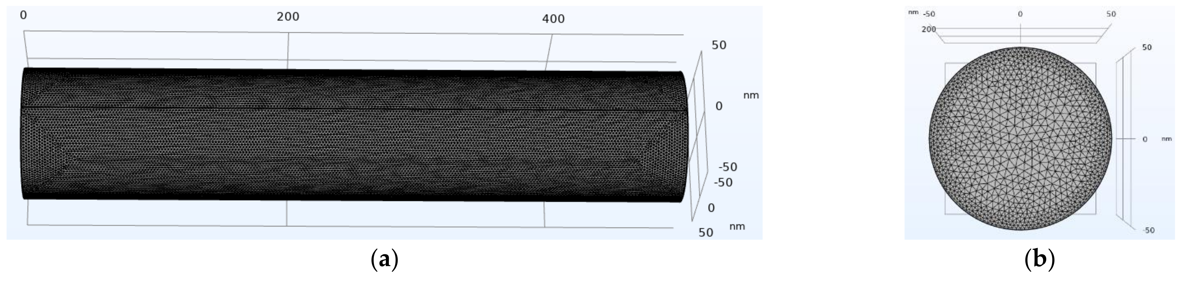
In the work, firstly, the finite element software COMSOL (5.5) was employed to establish a capillary model as shown in Figure 1, in which the length of the model was 500 nm, the radius was 50 nm, the fluid viscosity was 0.543 mPa$\cdot$s, and the fluid density is 703.5 g/cm³. They are coming from the properties of n-C8H18 at 20 degrees C and will be used in all the numerical models. The non-uniform triangular mesh was employed for mesh generation. The finer mesh was used near the solid wall surface while the coarser mesh was used in the central fluid area. The independence of the mesh was tested to ensure the reliability of the simulation results. The correctness of the model was verified by comparing the established COMSOL numerical model with the analytical solution at two conditions: with slip flow and without slip flow.

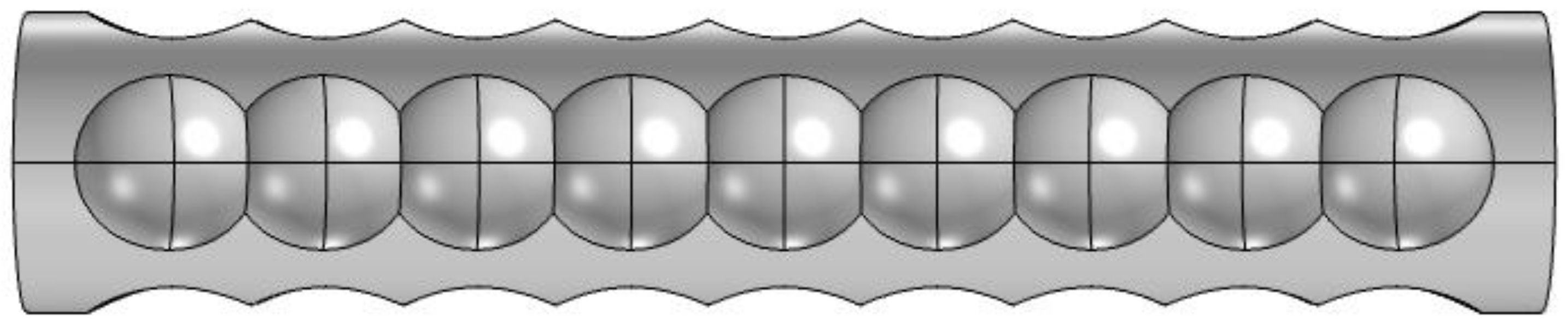
Then, balls with a diameter of 60 nm were evenly embedded on the outer circumference of the capillary model, so that the smooth inner wall became concave and convex, to simulate the roughness of the pore structure and a rough-wall tube model was established, as shown in Figure 2. The fluid flowing in the tube was comparatively analyzed considering the slip effect on the wall surface. The real slip length data was sourced from the literature [29], which had been obtained through a molecular dynamics simulation of the oil flow in quartzose pores.

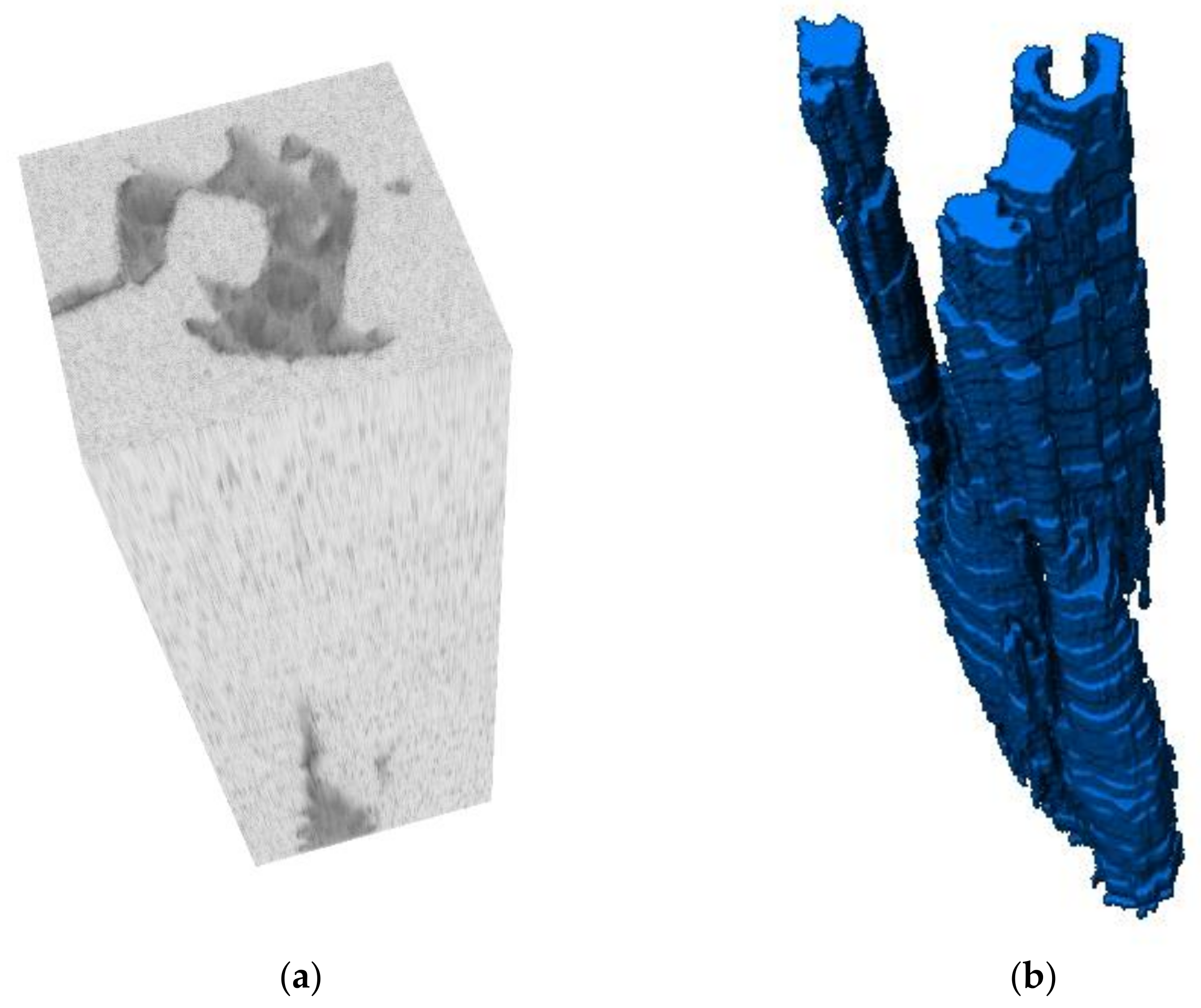
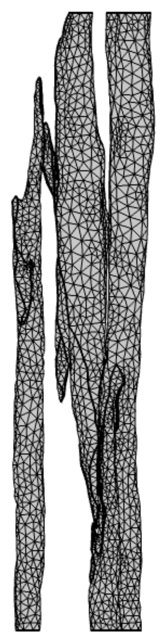
The actual shale oil core was selected coming from the Chang 7 Member of the Yanchang Formation, with porosity 3.1% and permeability 2.15 × 10⁻³ mD, and the oil flow in the pores was calculated and analyzed through importing the pore space reconstructed with CT scanning into COMSOL, in order to truly reflect the influence of the shale oil pore structure on seepage. The three-dimensional images of shale core samples were collected with Nano-CT scanning equipment from ZEISS Xradia, with a resolution of 64.2 nm/pixel. In the experiment, the small samples were taken from a large shale sample and then ground into a cylinder-like core with both ends polished flat. Since there was a difference in the grayscale between the central area and the surrounding boundary area of the scanned image, a cube part was extracted from the central area for further research to avoid errors. The software PerGeos was used for digital analysis, the two-dimensional image of the sample was obtained with a CT algorithm, on which the filter function was used to remove the noise. The obtained gray-scale image was converted into a binary black-and-white image by threshold function processing, in which black represented the pore space of the core and white represented the skeleton of the core. The three-dimensional structure of the core was reconstructed by superimposing all the data together, as shown in Figure 3.

The STL file was used to realize the data exchange between PerGeos and COMSOL. When the geometric shape of the pore was obtained, it was necessary to use the tool Generate Surface to generate the geometric surface of the pore space. If the pore structure was complex, it would be necessary to simplify the surface of the extracted pore. The large triangle was generated in the plane area, and the small triangle was generated in the high curvature area so that the details could be preserved and the simple triangle surface file could be exported. The surface editor module of the software PerGeos was employed to repair the surface details of the digital pore space model via human–computer interaction, including the repair of gaps and sharp corners, and the elimination of defects such as intersections, gaps, chamfers, co-planes, holes and overlapping edges, and, eventually, a triangular mesh with good quality was generated. Finally, the data was saved as an STL file that could be recognized by the finite element software COMSOL, to build a bridge between the geometric model of the digital core and the micro-seepage simulation. Figure 4 shows the surface mesh constructed by PerGeos, which can generate STL files. When an STL file is imported into the finite element software COMSOL, it is necessary to correct some simulated topologies geometrically, including the adjustment of the maximum angle, the maximum-plane adjacent angle and the minimum relative area and the removal of facets in the pore surface. Figure 5 is the mesh generation diagram of pores, in which the disconnected pores were removed in COMSOL. The length of the model is 390 nm.

Based on the two-fluid model, the effective boundary slip length was adopted to establish the mathematical seepage model on shale oil core scale, the theoretical correctness of which was verified with the results of the actual shale oil core displacement experiment.

3. Results and Discussion

When the boundary slip is not considered, the fluid flow in a circular tube conforms to the classical Poiseuille equation, and the formulae for its velocity distribution and flow rate are as follows:

$${\mu }_{HP}=-\frac{R^2}{4\mu }\frac{\Delta p}{L}\left(1-\frac{r^2}{R^2}\right)$$

(3)

$$\mathrm{Q}=\frac{\pi R^4}{8\mu }\frac{\Delta p}{L}$$

(4)

where L is the length of the capillary model, m; R is the radius of the capillary, m; Δp is the pressure difference, Pa.

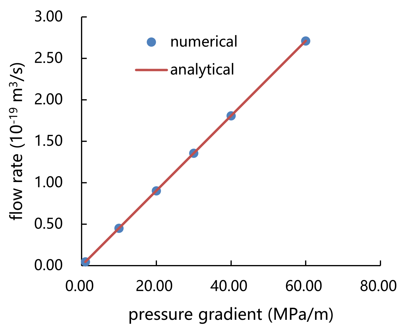
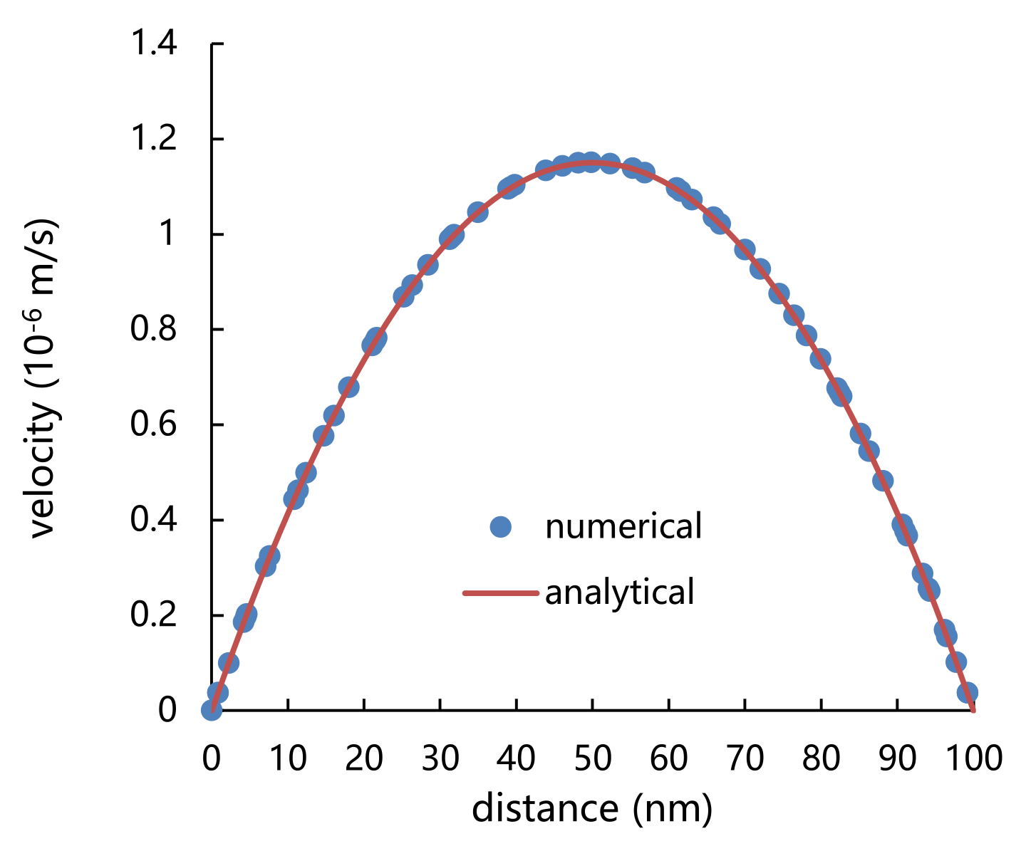
A constant pressure difference was set at both ends of the capillary as shown in Figure 1, and the Navier–Stokes equation was applied to the calculation domain to obtain the numerical solution, which was compared with the analytical solution to verify the correctness of the established COMSOL numerical model. It can be seen from Figure 6 and Figure 7 that the velocity distribution and flow rate obtained with the simulation are consistent with the results predicted by the analytical formulas, which verifies the effectiveness of this method.

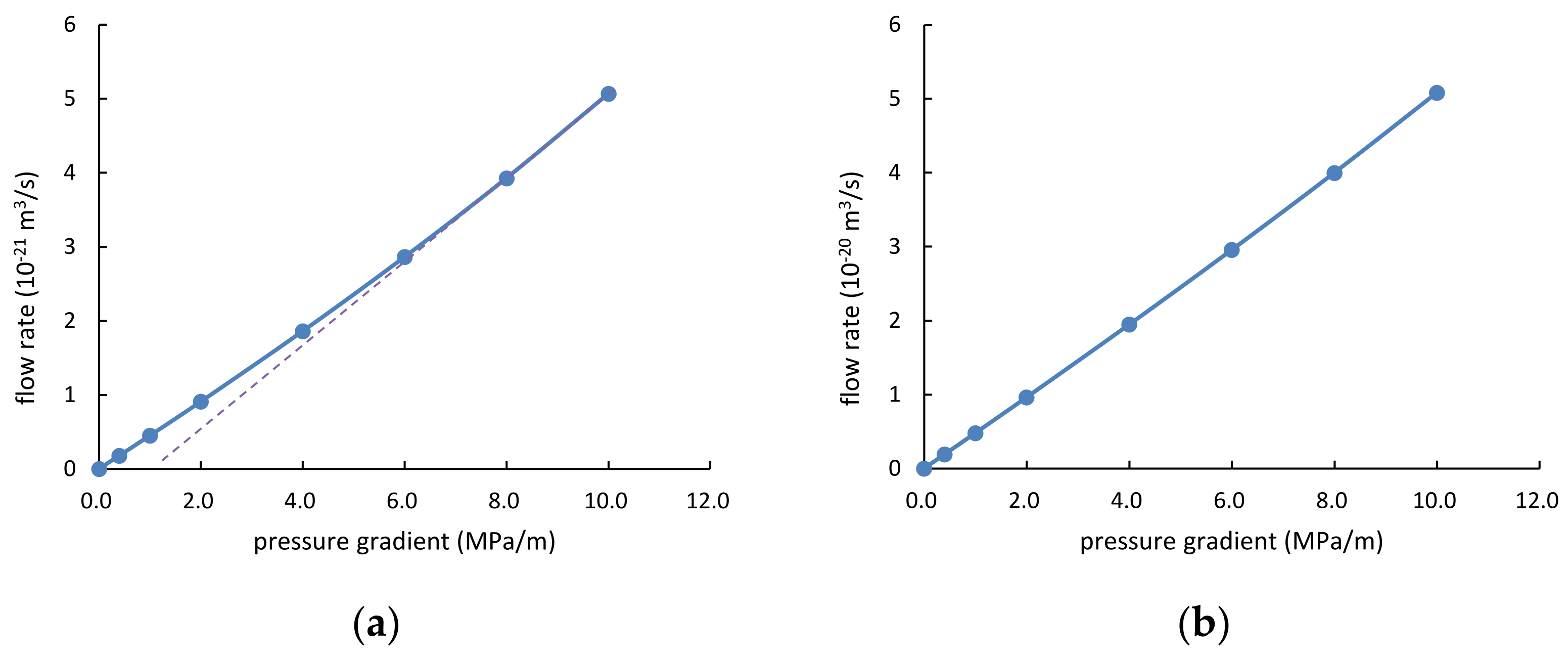
When the boundary slip is considered, the Poiseuille equation is as follows:

$$\mathrm{Q}=\frac{\pi R^4}{8\mu }\frac{\Delta p}{L}\left(1+4\frac{l_{\mathrm{st}}}{R}\right)$$

(5)

On the basis of the above COMSOL circular tube model, the velocity slip was considered at the boundary, and the slip length ($l_{\mathrm{st}}=5\mathrm{nm}$) was used to calculate the flow rate under different pressure gradients, as shown in Figure 8.

It can be seen in Figure 6, Figure 7 and Figure 8 that the numerical model established by COMSOL could perfectly match the analytical solution with or without consideration of the boundary slip. Additionally, it is also found that when the boundary slip is considered, the flow rate at the same pressure gradient is higher than that when the boundary slip is not considered.

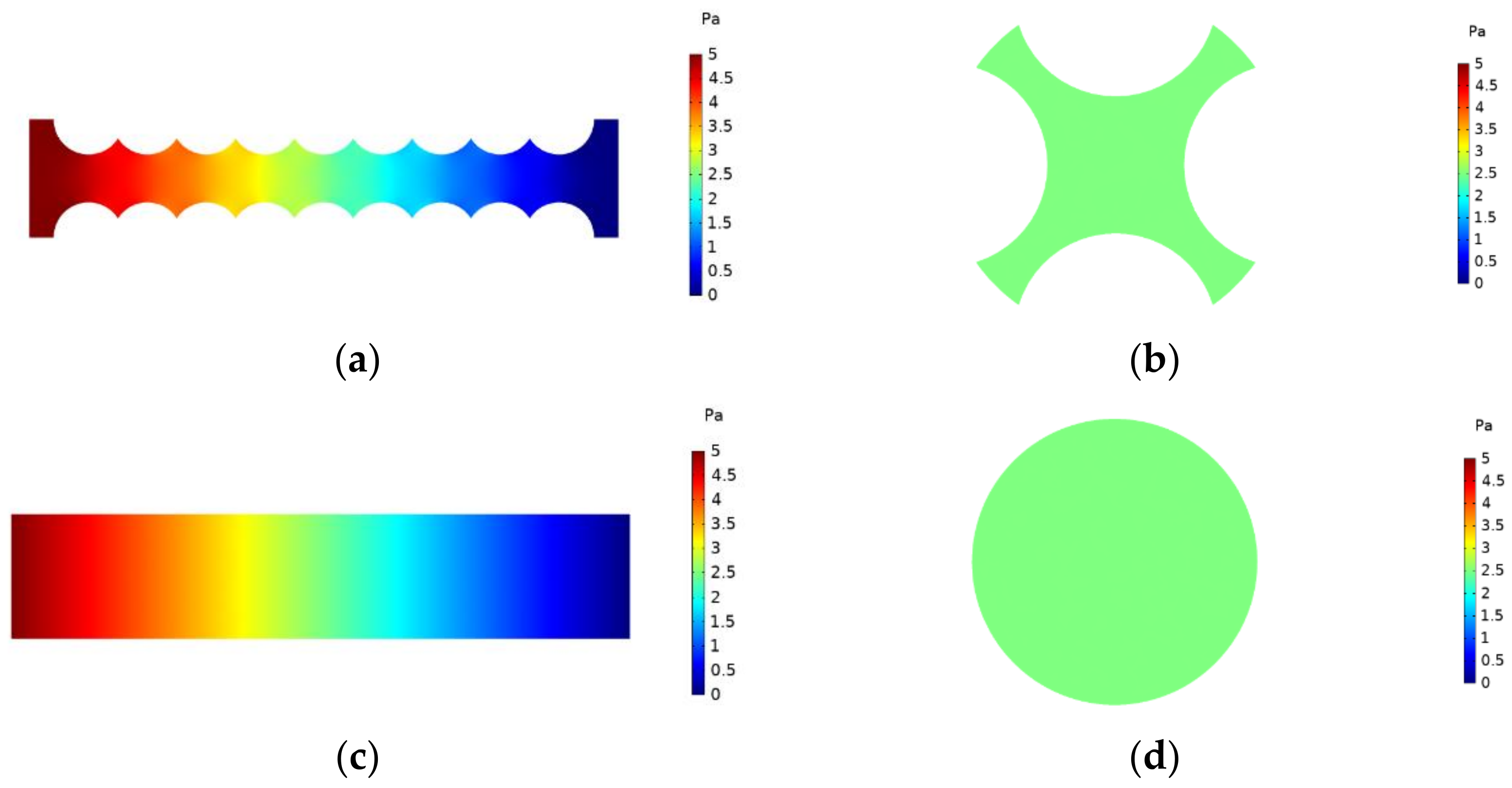
The real slip length obtained with a molecular dynamics simulation in the literature [29] (as shown in Figure 12) was used to analyze the flow law in the circular tube models shown in Figure 1 and Figure 2. The comparisons of velocity fields and pressure fields in the rough wall model and smooth wall model are shown in Figure 9 and Figure 10, respectively (with a pressure difference of 5 Pa). It can be seen that in the pores with a smooth wall surface, the distribution of the flow line was relatively straight, while in the pores with a rough wall surface, the uneven fluctuation of the inner wall made the flow line bent. Particularly, as the sections with low velocity on the wall surface increased, the seepage resistance increased, resulting in the decrease in the flow rate under the same pressure difference.

Figure 11 shows the relationship between the displacement pressure gradient and flow rate. It is obviously seen that the flow rate in the rough wall surface model was one order of magnitude lower than that in the smooth wall surface model under the same pressure gradient. Additionally, it is found that the relationship between the pressure gradient and the flow rate was no longer linear, and the flow rate increased nonlinearly with the pressure gradient until the relationship changed to be linear.

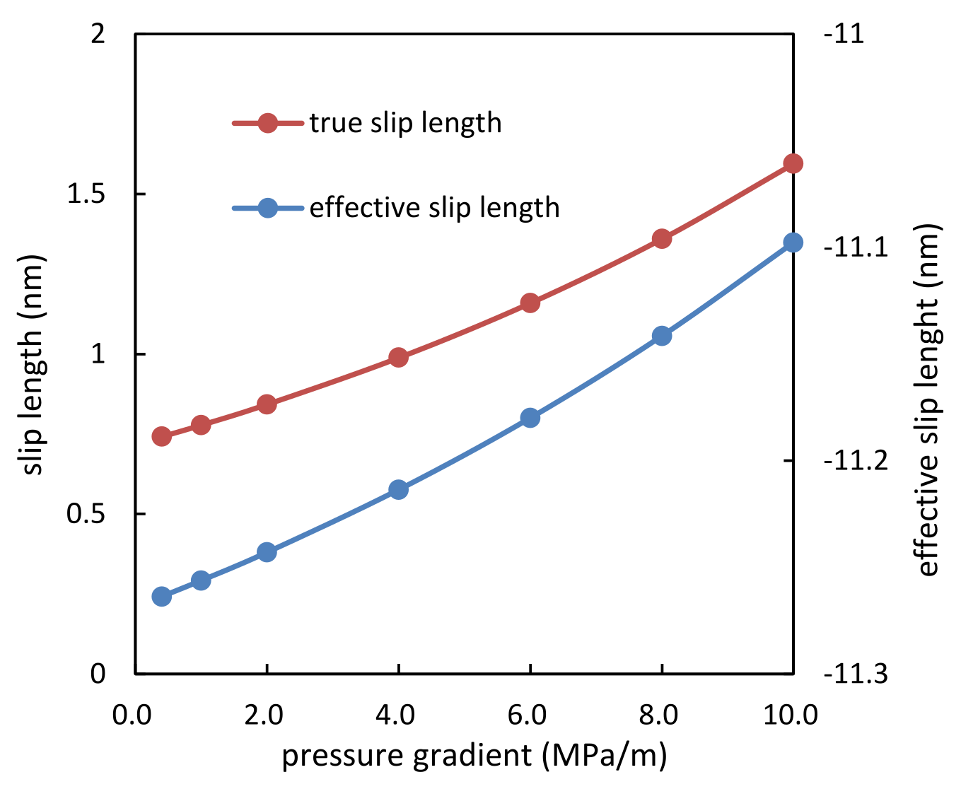
The real slip length $l_{\mathrm{st}}$ was replaced by the effective slip length $l_{seff}$, in order to better characterize the influence of the intra-pore structure variation on the fluid flow. The effective slip length can be expressed as:

$$l_{\mathrm{seff}}=\frac{R}{4}\left(\frac{8\mathrm{Q}\mu }{\pi R^4}\frac{L}{\Delta p}-1\right)$$

(6)

The effective slip length was used to comprehensively characterize the real boundary slip and the change of pore space. Figure 12 shows the comparison of two slip lengths. It can be seen that the effective slip length became negative after the variation of the pore structure was considered, which explained why the predicted flow rate was lower than that in the smooth wall model.

Figure 12. Comparison of slip lengths.

Figure 12. Comparison of slip lengths.

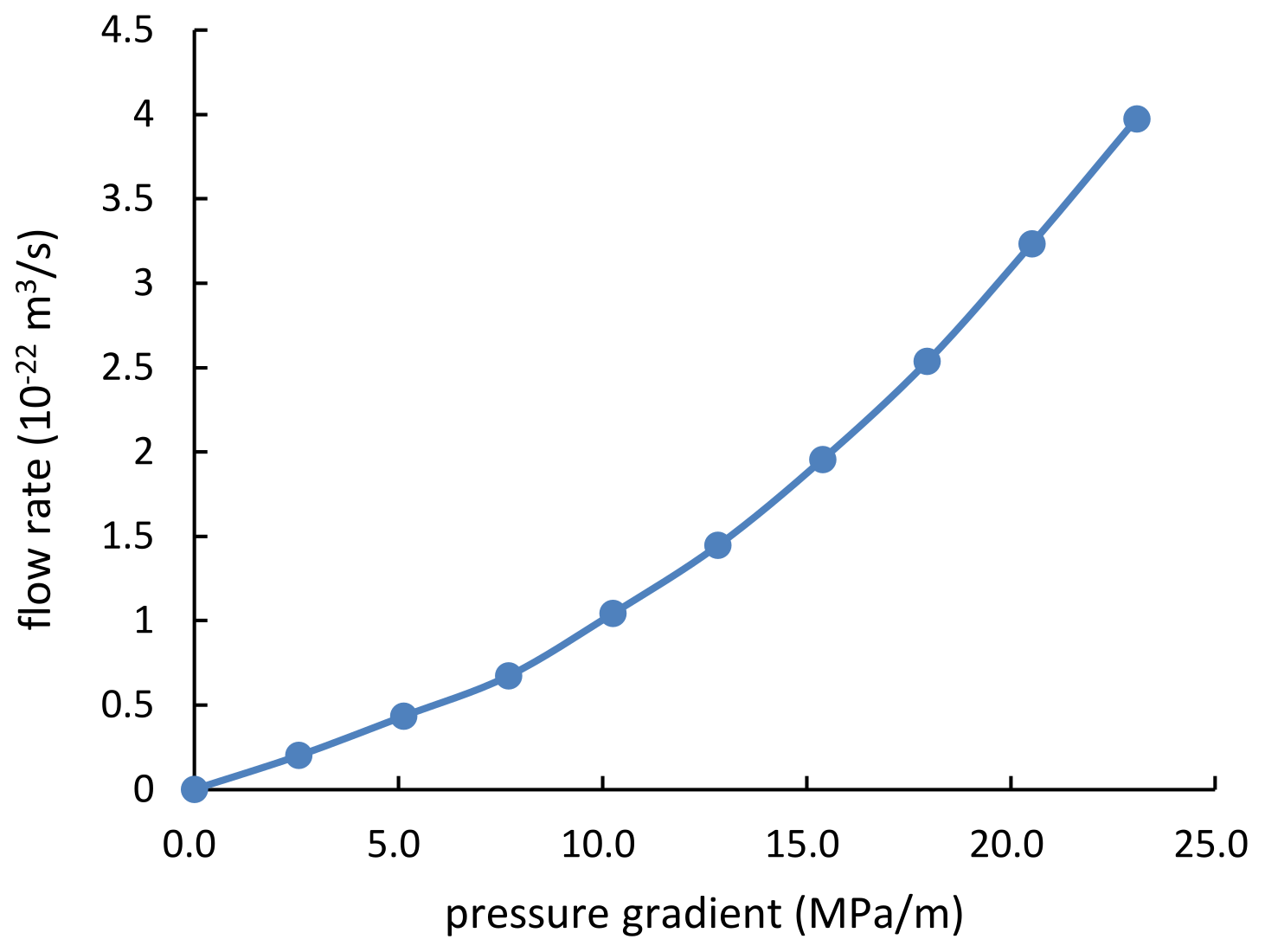
The real pore structure shown in Figure 5 was used to calculate the flow rate of shale oil. Figure 13 shows the flow rate curve under different pressure gradients. The shape of the seepage curve was very close to the results of the core displacement experiment. Although the boundary slip was considered in the calculation process, the calculation results still showed a concave nonlinear increase, suggesting that the complexity of the pore structure greatly affected the shape of the seepage curve.

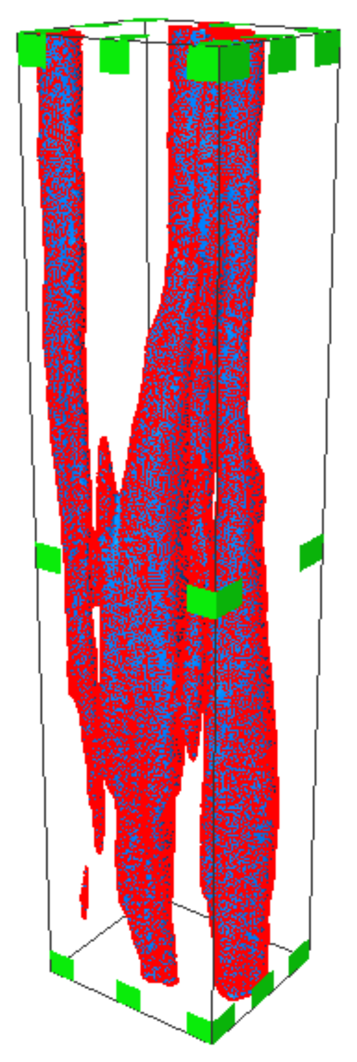
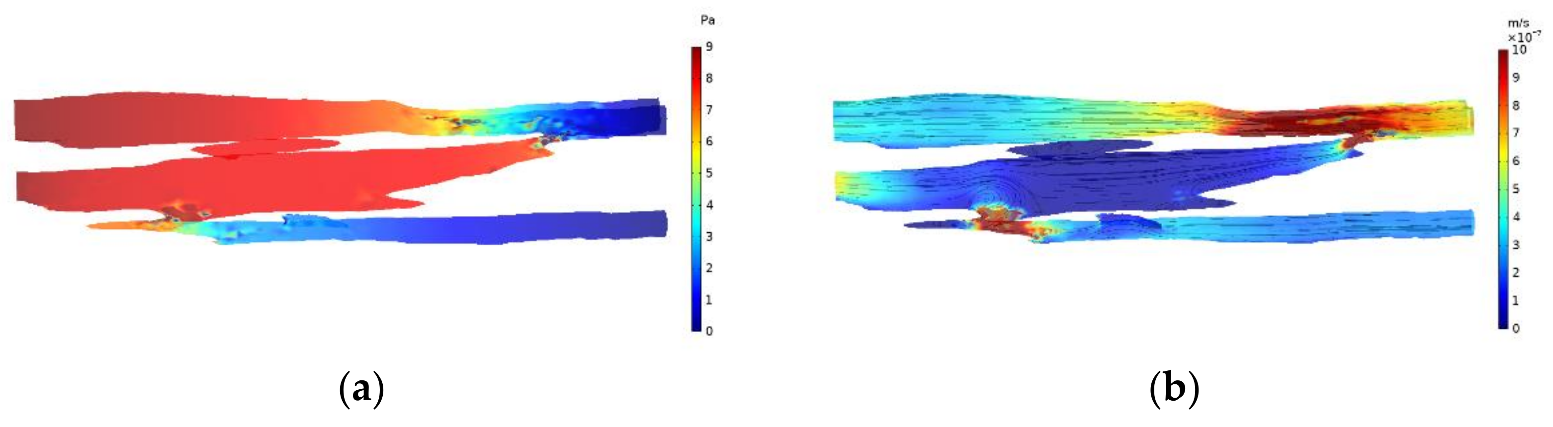
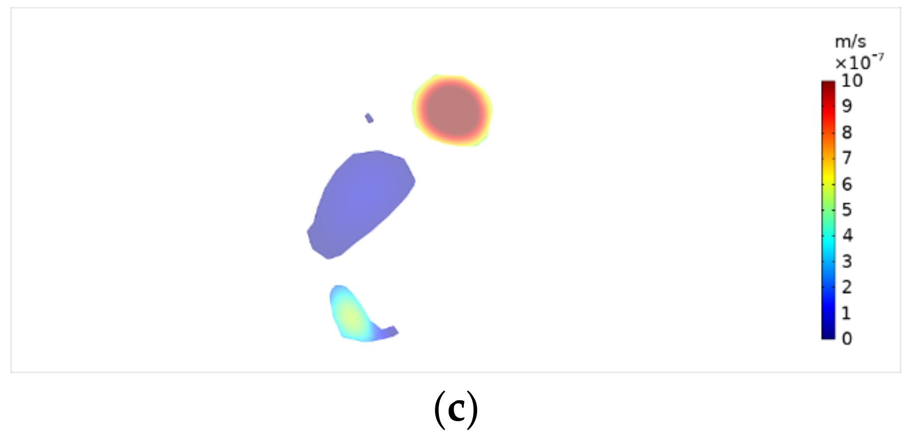
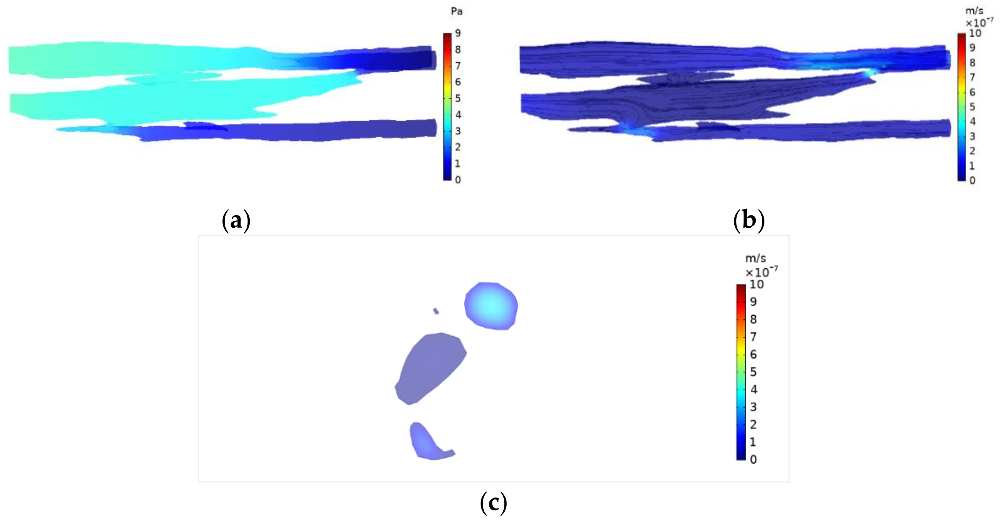
The distributions of the pressure field and the velocity field in this model are shown in Figure 14 and Figure 15, respectively. It can be seen from the figures that the area of pores at the entrance was relatively large, but the fluid needed to pass through a small area of pores at the exit in the upper part of the model, which resulted in a high pressure in the middle part of the model and a low flow rate. The connection between pores greatly affected the seepage law. It was found that by comparing the two displacement pressure differences with the increase in the displacement pressure difference, the proportion of flow in pores gradually increased, and the flow line gradually tended to be stable, so the seepage curve showed a change from nonlinear to relatively linear.

It can be seen from the above analysis that even when the wall slip effect was considered, the complexity of pore structure still led to the change of the seepage curve from the nonlinear section to the linear section. In consideration of the differences of physical properties between the boundary fluid and the bulk fluid caused by the confinement effect in the micro-nano pores, the effective boundary slip length was used to comprehensively characterize the influence of the real slip length and pore structure on the seepage, and the motion equation of shale oil has been established to reasonably characterize the seepage of shale oil in the complex pore structure.

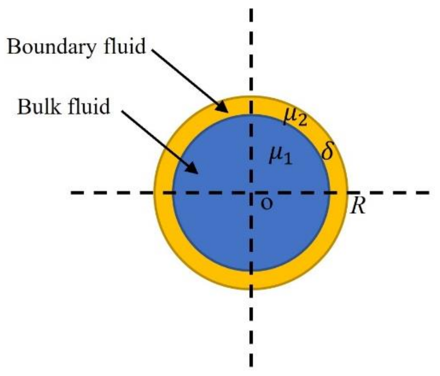
As shown in Figure 16, the fluid flowed steady in the capillary tube with a radius R and a length L, and the pressure difference between the two ends was $\Delta p$. Because of the interaction between the nanotube wall and the fluid, the properties of the boundary layer fluid and the bulk fluid were different. It is supposed that the viscosity and velocity for the bulk fluid are ${\mu }_1$, and $u_1$, respectively, and the viscosity, thickness, and velocity of the boundary fluid are ${\mu }_2$, $\delta$ and $u_2$, respectively, the mathematical model that accounts for the boundary slip will be as follows:

$$\frac{{\mu }_1}{r}\frac{\partial }{\partial r}\left(r\frac{\partial u_1}{\partial r}\right)=\frac{\Delta p}{L}(0\le r\le R-\delta )$$

(7)

$$\frac{{\mu }_2}{r}\frac{\partial }{\partial r}\left(r\frac{\partial u_2}{\partial r}\right)=\frac{\Delta p}{L}(R-\delta \le r\le R)$$

(8)

$${\left.\frac{\partial u_1}{\partial r}\right|}_{r=0}=0$$

(9)

$${\left.-l_{st}\frac{\partial u_2}{\partial r}\right|}_{r=R}={\left.u_2\right|}_{r=R}$$

(10)

The velocity and shear stress at the interface of boundary fluid and bulk fluid are continuous, then

$${\left.u_1\right|}_{r=R-\delta }={\left.u_2\right|}_{r=R-\delta }$$

(11)

$${\mu }_1{\left.\frac{\partial u_1}{\partial r}\right|}_{r=R-\delta }={\mu }_2{\left.\frac{\partial u_2}{\partial r}\right|}_{r=R-\delta }$$

(12)

The general solution of the model is as follows:

$$u_1=-\frac{\Delta p}{L}\frac{r^2}{4{\mu }_1}+c_1(0\le r\le R-\delta )$$

(13)

$$u_2=-\frac{\Delta p}{L}\frac{r^2}{4{\mu }_2}+c_2(R-\delta \le r\le R)$$

(14)

Combination of Equations (10) and (14) results in:

$$c_2=\frac{\Delta p}{L}\frac{R^2+2R{l}_{st}}{4{\mu }_2}$$

(15)

Therefore,

$$u_2=-\frac{\Delta p}{L}\frac{r^2}{4{\mu }_2}+\frac{\Delta p}{L}\frac{R^2+2R{l}_{st}}{4{\mu }_2}=\frac{\Delta p}{L}\frac{R^2-r^2+2R{l}_{st}}{4{\mu }_2}$$

(16)

After combining Equations (11) and (16), therefore,

$$c_1=\frac{\Delta p}{L}\frac{{\mu }_1{R}^2+\left({\mu }_2-{\mu }_1\right){\left(R-\delta \right)}^2+2R{\mu }_1{l}_{st}}{4{\mu }_1{\mu }_2}$$

(17)

$$u_1=\frac{\Delta p}{L}\left[\frac{1}{4{\mu }_2}\left(R^2-\frac{{\mu }_2}{{\mu }_1}{r}^2\right)+\frac{R{l}_{st}}{2{\mu }_2}+\frac{\left({\mu }_2-{\mu }_1\right){\left(R-\delta \right)}^2}{4{\mu }_1{\mu }_2}\right]$$

(18)

Therefore, the flow rate is:

$$\begin{array}{cc}\hfill & Q=2\pi \left(\underset{0}{\overset{R-\delta }{\int }}r{u}_1\mathrm{d}r+\underset{R-\delta }{\overset{R}{\int }}r{u}_2\mathrm{d}r\right)=\frac{\pi R^4}{8{\mu }_1}\frac{\Delta p}{L}\left[{\left(\frac{R-\delta }{R}\right)}^4\left(1-\frac{{\mu }_1}{{\mu }_2}\right)+\frac{{\mu }_1}{{\mu }_2}\left(1+\frac{4l_{st}}{R}\right)\right]\hfill \\ \hfill & =\frac{\pi R^4}{8{\mu }_1}\frac{\Delta p}{L}\left[\left(1-\frac{4\delta }{R}+\frac{6{\delta }^2}{R^2}-\frac{4{\delta }^3}{R^3}+\frac{{\delta }^4}{R^4}\right)\left(1-\frac{{\mu }_1}{{\mu }_2}\right)+\frac{{\mu }_1}{{\mu }_2}\left(1+\frac{4l_{st}}{R}\right)\right]\hfill \\ \hfill & \approx \frac{\pi R^4}{8{\mu }_1}\frac{\Delta p}{L}\left(1-\frac{4\delta }{R}+4\frac{{\mu }_1}{{\mu }_2}\frac{\delta }{R}+4\frac{{\mu }_1}{{\mu }_2}\frac{l_{st}}{R}\right)\hfill \\ \hfill & =\frac{\pi R^4}{8{\mu }_1}\frac{\Delta p}{L}\left(1-\frac{4\delta }{R}+4\frac{{\mu }_1}{{\mu }_2}\frac{\delta }{R}+4\frac{{\mu }_1}{{\mu }_2}\frac{l_{st}}{R}\right)\hfill \end{array}$$

(19)

After defining the effective slip length $l_{s\mathrm{eff}}$, then:

$$\mathrm{Q}=\frac{\pi R^4}{8{\mu }_1}\frac{\Delta p}{L}\left(1+4\frac{l_{s\mathrm{eff}}}{R}\right)$$

(20)

Therefore,

$$l_{s\mathrm{eff}}=\left[\delta \left(\frac{{\mu }_1}{{\mu }_2}-1\right)+\frac{{\mu }_1}{{\mu }_2}{l}_{st}\right]$$

(21)

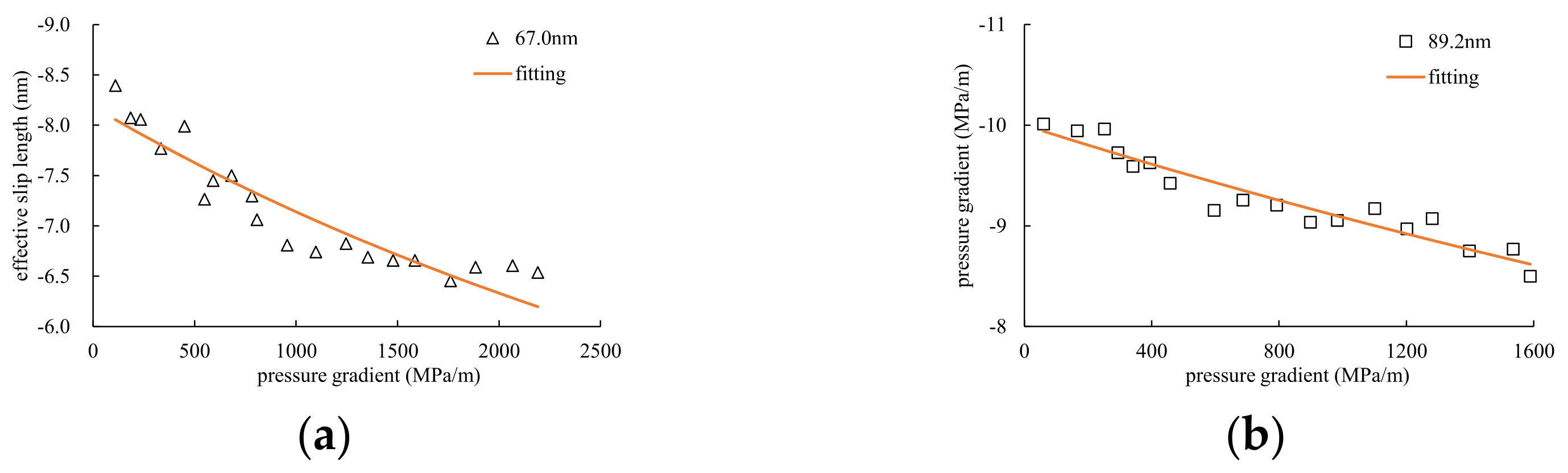
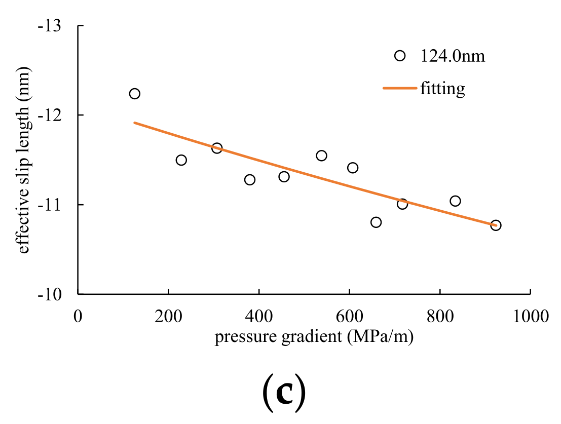
An analysis was conducted by Hu et al. [30] on the flow characteristics of water in nanometer tubes, in which deionized water was selected to conduct displacement experiments in alumina membranes with pore sizes of 67.0 nm, 89.2 nm, and 124 nm under 0.01~0.2 MPa. It was found that the slip length was a function of the pressure gradient. Based on the experiment results, the following equation is proposed to characterize the relationship between the slip length and the pressure gradient.

$$l_{s\mathrm{eff}}=\frac{a}{\left|\nabla p\right|+b}$$

(22)

The experiment results were fitted with the above relationship, as shown in Figure 17. It can be seen that Equation (22) well characterized the relationship between slip length and pressure gradient.

After substituting Equation (22) into Equation (20),

$$\mathrm{Q}=\frac{\pi R^4}{8{\mu }_1}\nabla p\left(1+\frac{a^{’}}{\left|\nabla p\right|+b}\right)$$

(23)

where $a^{’}=4a/R$. It is considered that there is no threshold pressure gradient, therefore, when $\left|\nabla p\right|=0$,

$$1+\frac{a^{’}}{\left|\nabla p\right|+b}=0$$

(24)

So, $a^{’}=-b=-m$, then

$$\mathrm{Q}=\frac{\pi R^4}{8{\mu }_1}\left(1-\frac{m}{\left|\nabla p\right|+m}\right)\nabla p$$

(25)

The real rock is equivalently considered as a bundle of capillary tubes consisting of n tubes with a radius R per unit area, the flow rate passing through the rock surface with an area A will be calculated with the equation below:

$$\mathrm{Q}=\mathrm{nA}\frac{\pi R^4}{8{\mu }_1}\left(1-\frac{m}{\left|\nabla p\right|+m}\right)\nabla p$$

(26)

According to $\varphi =\mathrm{n}\pi R^2$, $K=\varphi R^2/8$, therefore,

$$\mathrm{Q}=\frac{K}{{\mu }_1}\mathrm{A}\left(1-\frac{m}{\left|\nabla p\right|+m}\right)\nabla p$$

(27)

where Q is the flow rate, K is the permeability, ${\mu }_1$ is the fluid viscosity, $\nabla p$ is the pressure gradient, and m is the nonlinear flow parameter accounting for the influences of geometry variation, pore confinement and slip on flow.

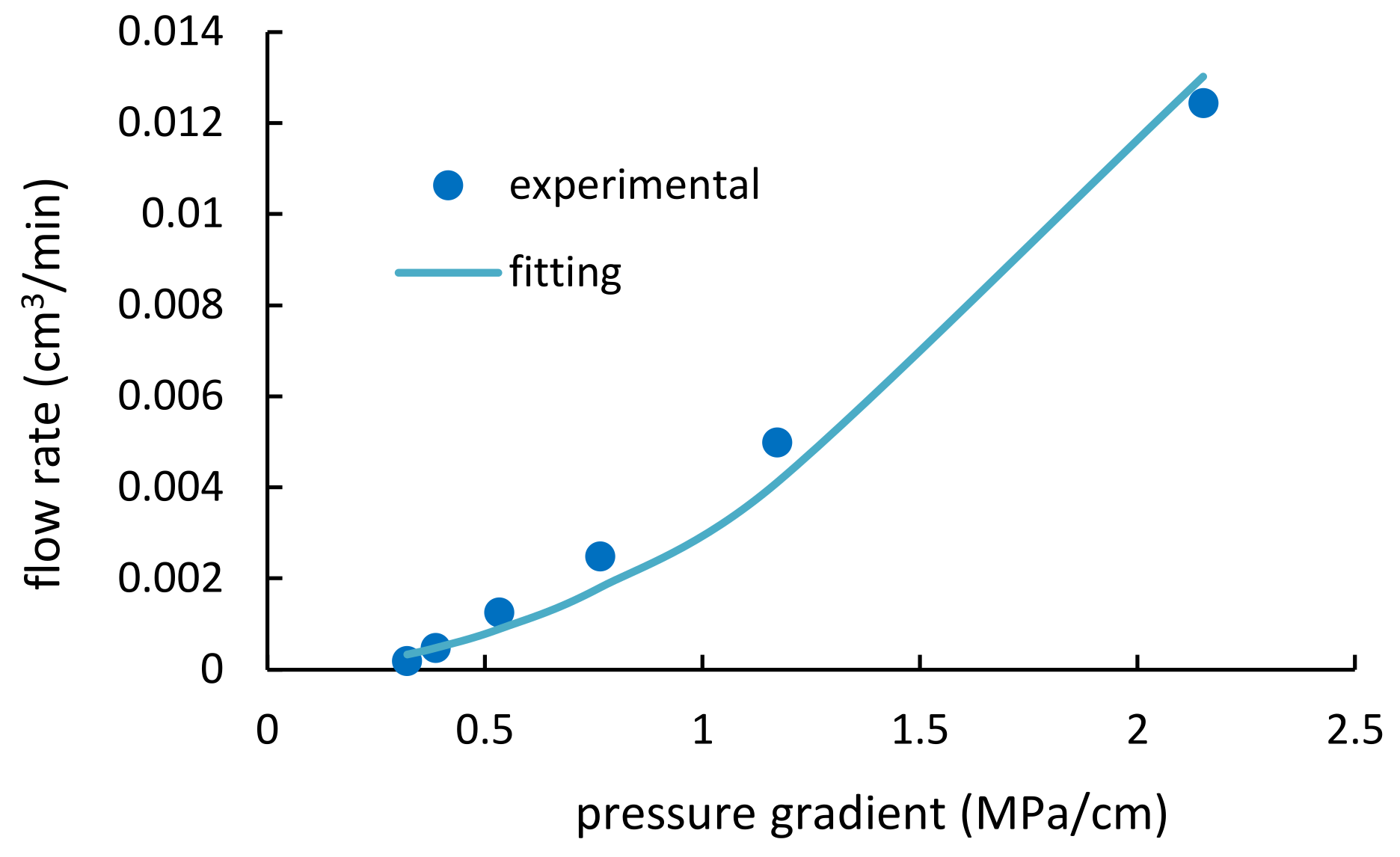
The seepage law was extended from the pore scale to the core scale based on the slip theory so far in this paper. Figure 18 shows the results of the displacement experiment with Jiyang shale oil cores. The displacement fluid was oil, and the experimental data came from the literature research [6]. In the experiment, the permeability of the core was 0.154 mD and the oil viscosity was 10.13 mPa$·$s. The seepage curve of the core was fitted by Equation (27), with a fitting coefficient m = 14.29 MPa/cm. It was found that this equation could well characterize the characteristics of the seepage curve, and the fitting degree exceeded 0.9749, suggesting that the derived seepage model could reflect the seepage characteristics of shale oil.

4. Conclusions

Based on the software COMSOL, a capillary model with a rough wall surface considering the slip effect has been established. Then, the real pore structure of the shale oil core was reconstructed with CT scanning to simulate the microscopic seepage process of shale oil in the real pore structure. Finally, according to the two-fluid model, the effective slip length was used to comprehensively characterize the pore structure change and the real wall surface slip, and to establish the mathematical model for describing shale oil seepage. The following conclusions can be drawn:

(1)

Pore structure seriously affected the characteristics of the seepage curve. The studies showed that the fluid in the pores increasingly participated in the flow with the increase in displacement pressure, showing a changing trend of relationship from nonlinearity to linearity.

(2)

The established shale oil seepage mechanism model could reflect the characteristics of nonlinear change, and the verification was made with the actual displacement data, suggesting the correctness of the model. However, the proposed model is under the assumption of no threshold pressure gradient, which is not applicable in the threshold pressure gradient analysis.