Abstract
Past studies of microgrids have been based on measurements of fuel consumption by generators under static loads. There is little information on the fuel efficiency of generators under time-varying loads. To help analyze the impact of time-varying loads on optimal generator operation and fuel consumption, we formulate a mixed-integer linear optimization model to plan generator and energy storage system (ESS) operation to satisfy known demands. Our model includes fuel consumption penalty terms on time-varying loads. We exercise the model on various scenarios and compare the resulting optimal fuel consumption and generator operation profiles. Our results show that the change in fuel efficiency between scenarios with the integration of ESS is minimal regardless of the imposed penalty placed on the generator. However, without the assistance of the ESS, the fuel consumption increases dramatically with the penalty imposed on the generator. The integration of an ESS improves fuel consumption because the ESS allows the generator to minimize power output fluctuation. While the presence of a penalty term has a clear impact on generator operation and fuel consumption, the exact type and weight of the penalty appears insignificant; this may provide useful insight for future studies in developing a real-time controller.
1. Introduction
Demand for energy is increasing significantly worldwide. This is particularly true in the United States Department of Defense (DoD), which is the largest consumer of energy in the federal government [1]. As warfighting transitions into the cyber and space domains, energy “has been and will remain a fundamental enabler of military capability” according to the United States (US) Office of Assistant Secretary of Defense for Energy, Installations, and Environment [2]. Military organizations need reliable and sustainable microgrid power systems to effectively generate energy required for deployed military operating bases.
Microgrid Operations
When temporary military bases are built in forward operating areas such as the Middle East, self-sustainability is one of the most important features to take into account, as one cannot rely on local power grids. An islanded microgrid is formed when an electrical grid is capable of operating in isolation from the main grid [3]. Islanded microgrid operations are very common in military settings.
An islanded microgrid typically consists of generators, an energy storage system (ESS), and loads that need to be met. A centralized controller calculates the optimal power flow balance between the generators and the ESSs [4], as shown in Figure 1. This ensures that all critical loads are met during all microgrid operating modes [5,6]. As a result, the controller improves reliability, reduces cost, and diversifies power generation. As microgrids are intended to be self-sufficient, the ESS is one of the primary ways to ensure that the system is stabilized against fluctuating loads and unmanaged energy sources [5].
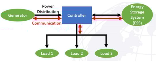
Figure 1.
Notional microgrid controller flowchart with power distribution and communication flow. Adapted from Craparo and Sprague [7].
A key function of the controller is to determine the optimal power flow among the generators, ESSs, and loads in such a way as to satisfy demand while minimizing fuel consumption. To accomplish this, the controller must model fuel consumption as a function of generator output. Existing studies primarily utilize fuel efficiency (or consumption) profiles based on static generator output (e.g., [8,9,10,11]). To build these profiles, generator manufacturers run generators at various constant loads for long periods of time and measure the resulting fuel consumption [12]. In practice, loads encountered on islanded microgrids are generally not constant but instead vary over time, often quite rapidly. To our knowledge, no data exist quantifying generator efficiency under time-varying loads. However, data from other settings (e.g., automotive fuel efficiency) suggest that fluctuating loads may significantly degrade generator efficiency [13].
In this study, we develop an optimization-based approach to model loss of efficiency with fluctuating generator output and to optimally plan generator and ESS operations in such a way as to minimize fuel consumption while satisfying demand. To our knowledge, this is the first work to consider efficiency losses due to fluctuating generator output. In addition to potential fuel savings, reducing generator output fluctuations can improve generator stability as well as operational lifetime [14,15]. Additionally, any potential fuel savings at an islanded microgrid are generally magnified when one considers the fully burdened cost of fuel, accounting for the monetary and energy costs associated with transporting fuel to the location at which it will be consumed. Ref. [8] provides an overview of this cost in military settings, including both the energy cost and cost in human life to transport fuel to a forward operating theater.
2. Background and Literature Review
Previous studies explore different approaches to vary the architecture of microgrids, find unique ways to optimally schedule energy distribution, and formulate optimization models. It is imperative to optimize microgrids to be cost effective and reliable to deploy based on measure of fuel consumption.
2.1. Microgrid Architecture Variation
The two main energy resources that make up an islanded microgrid architecture are the generator(s) and the ESS. It is important to determine the correct size of these resources in a microgrid to meet the power demand at any given time [16,17]. One way to properly size microgrid components is in accordance to the peak-load demand criteria [18]. In addition to using peak-load demand data, research has been conducted on integrating an optimal hybrid photovoltaic (PV)/wind/diesel generating system combination identified by a sizing algorithm based on power supply availability and power system design specifications [19].
Building off of a rudimentary sizing algorithm using past daily and seasonal load fluctuation, a more sophisticated dynamic energy flow model is used to determine the appropriate size of the microgrid components [20]. Then, past weather information such as solar and wind data are utilized to maximize the microgrid’s “islanding time”, which is defined as the time the microgrid can operate in a self-sufficient manner without external fuel supplies or connection to a main power grid [21].
An ESS sizing methodology uses a mixed-integer linear program (MILP) to choose an optimal storage size by taking initial investment costs and microgrid operating costs into account [22]. Similarly, some researchers have taken a more economic approach by introducing a cost–benefit analysis using forecast data to minimize total microgrid costs while maximizing the benefits from the respective storage size through an MILP technique [23].
2.2. Optimal Energy Scheduling Techniques
Optimal energy scheduling improves energy utilization while minimizing generator fuel consumption costs in a microgrid. An initial optimal energy scheduling technique was used to show that microgrid with ESS saves a significant amount of fuel compared to a microgrid without an energy storage unit [24]. Indeed, multiple studies have identified the ESS as a key component to ensure cost reduction [24,25]. Energy scheduling is especially important when ESSs are introduced into the microgrid architecture, as the system has the ability to store additional power for future use [22,23]. To reduce fuel cost and increase fuel efficiency, load scheduling becomes a crucial addition to the controller algorithm.
Another way to minimize fuel cost is to implement a day-ahead scheduling optimization technique for various microgrid operation modes such as utility grid-connected mode and off-grid operation mode [25]. Some work in day-ahead scheduling incorporates weather forecast data and models its impact on renewable production [26,27].
Instead of modeling a microgrid as a single entity, the particle swarm optimization (PSO) technique models the energy resources as individual particles that are parallel with each other, which creates a large network made up of many entities [28,29]. The parallel modeling technique enables shorter computation time when compared to a general MILP approach. The PSO optimization approach reduces computation time while minimizing energy production expense [29].
Ref. [30] considers the optimal scheduling of a diesel generator and an ESS, where the ESS is modeled using a detailed nonlinear model. They address the resulting planning problem with a combination of MILP and PSO. Ref. [31] models an islanded microgrid using a Markov decision process framework and then uses approximate dynamic programming to solve the resulting schedule optimization problem, while [32] considers the problem of placing distributed generators in such a way as to maximize efficiency and reliability.
2.3. Fuel Consumption Minimization
The main goal in most islanded microgrid research is to minimize fuel consumption, which often corresponds to maximizing generator efficiency. A common approach to quantify fuel consumption is using a cost optimization scheme of various power-sharing techniques to share the load between energy resources in a microgrid [33]. On highly nonlinear power-sharing schemes, linear, nonlinear, and dynamic strategies have sought to maximize microgrid efficiency [20,22,24,25,33].
Power-sharing techniques have been used to determine if additional electrical loads with expensive operating costs would effect the generator fuel consumption [10]. Other studies have minimized fuel consumption by integrating additional and various combinations of energy resources such as PV cells, batteries, and generator cycling in a microgrid architecture [34]. As fuel consumption is an important measure of performance, the goal of this paper is to minimize fuel consumption while ensuring that the power demand is efficiently met.
Some researchers have considered microgrids in settings other than strictly land-based. For instance, Ref. [35] considers shipboard microgrids and propose a hierarchical coordinated control approach to effectively manage the distinct operating modes inherent in these systems; Ref. [36] studies the hybridization of railway vehicles as a potential means to improve efficiency while satisfying various operational constraints. They demonstrate the potential for significant emmissions reduction by incorporating a properly sized ESS.
2.4. Novel Contribution and Organization
To our knowledge, all previous studies, including those in our literature review, have modeled generator fuel efficiency based on fuel curves derived by measuring fuel efficiency under static loading conditions (e.g., [12]). Experience from other domains (e.g., automotive) suggests that generator efficiency may be significantly degraded under dynamic load conditions such as those observed in microgrid operations [13]. To study the potential impact of this degradation, we introduce a generator penalty term designed to model a loss of efficiency as the generator output fluctuates. We include an ESS in our notional microgrid to allow the generator to produce a more constant output, despite fluctuating demand.
We first consider a linear approach where the fractional change in generator power is multiplied by a predefined scalar penalty coefficient and added to the cumulative fuel consumption. Second, we use a piecewise linear approach to vary the penalty coefficient based on the fractional change in generator power.
This paper is organized as follows. Section 3 describes our microgrid architecture and MILP optimization model. Section 4 exercises the model on a case study and highlights important insights. Section 5 presents the conclusion and final thoughts from this study as well as various recommendations for future research areas.
3. Methodology
This section describes our MILP optimization model of a forward operating base(FOB) microgrid, where the primary objective is to minimize the overall generator fuel consumption while satisfying a required power demand. Our microgrid equipment consists of a fuel-based generator and an ESS, and we exercise our model using power demand data collected from a US FOB located in the Middle East [37].
The MILP acts as a rudimentary power system controller which controls the power flow between the generator and ESS to satisfy the demand. Figure 1 depicts our controller architecture, including the power flow and communication flow. The controller maintains communication between the three separate components; however, power is only produced by the generator. This power may satisfy the demand directly or charge the ESS. The ESS may discharge power to meet demand.
3.1. Microgrid Architecture
This section describes the components of our notional FOB microgrid, as shown schematically in Figure 1.
3.1.1. Fuel-Based Generator
We model a 60 kilowatt (kW) Advanced Medium Mobile Power Sources (AMMPS) generator. This is a US Army-authorized power-generating unit that replaces the second generation Tactical Quiet Generator (TQG). We obtained steady-state generator fuel consumption data for four power settings, shown in Figure 2, from the US Army Base Camp Integration Lab [38].
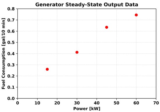
Figure 2.
Steady-state fuel consumption data from a 60 kW AMMPS generator at four distinct operating regions obtained from previous studies [38].
3.1.2. Energy Storage System
We model a 25 kilowatt-hours (kWh) ESS with a maximum charge rate and discharge rate of 20 kW with 90% round-trip efficiency (RTE); these values approximate the characteristics of a lithium-ion battery [39]. We constrain the ESS to maintain a state of charge (SOC) between 20% and 80% in order to prolong the lifespan of the ESS [40,41]. We initialize the ESS to an SOC of 50% in the first time period to simulate a continuously operating power system.
3.2. Optimization Model
The overall objective of the MILP optimization model is to minimize generator fuel consumption while satisfying demand in each time period t in T. Demand may be satisfied by the generator, the ESS, or some combination of the two. Additionally, the generator can produce power exceeding the demand, and the additional power charges the ESS. We denote the power produced by the generator in time step t as , the power used to charge the ESS (battery) as , and the power discharged from the battery as . Then, the power balance equation is
where is the discharge efficiency of the battery. We express the battery SOC as a percentage of the maximum charge and calculate it as
where represents the charging efficiency of the battery and represents the length of our time step in hours.
We restrict our generator to operate between a minimum power output of kW and a maximum power output of kW:
Similarly, we define and as the maximum charge and discharge rates of the battery, and we constrain the battery to maintain an SOC between and :
To simulate ongoing operations and avoid end-of-horizon effects, we require that the final SOC is equal to the initial SOC:
The overall objective of the MILP optimization model is to minimize the fuel consumed by the generator. As shown in Figure 3, we use a least-squares linear fit to represent steady-state fuel consumption based on our data. The linear fit is defined by its slope and intercept, where is the fuel consumption slope of and is the fuel consumption intercept of . This steady-state fuel consumption is typically the only fuel consumption term accounted for in previous studies, as shown in Equation (8). Figure 4 shows the resulting steady-state generator efficiency curve.
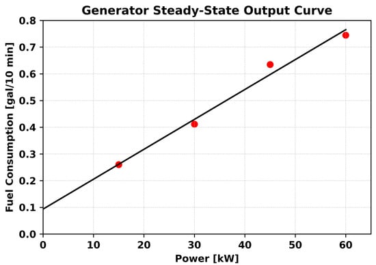
Figure 3.
Fuel consumption of a 60 kW AMMPS generator with a linear fit based on generator steady-state power output data.
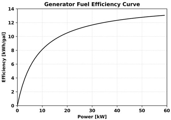
Figure 4.
Fuel efficiency curve of a 60 kW AMMPS generator based on generator steady-state power output data.
To address our primary study objective, we include an additional “penalty term” to capture the efficiency loss incurred when the generator output power fluctuates rapidly from time period to time period:
We now describe our methodology for calculating .
3.3. Generator Penalty Concept
We consider two different approaches to calculate the “penalty term” in Equation (9). First, we calculate as a linear function of the (approximate) fractional change in generator output from time period to time period. Second, we calculate as a piecewise linear function of the fractional change in generator output.
3.3.1. Linear Penalty Approach
First, we express as a linear function of the fractional change in generator output from one time period to the next. Let denote the fractional change in generator output from time period to time period t. Then, is exactly calculated as
In order to formulate a linear optimization model, we instead calculate an approximate value for . First, we calculate the absolute change in generator output for all t in T using the linear constraints
where we rely on the fact that fluctuations are penalized in our objective function, and thus, the solver chooses the smallest feasible value for , given the values of and .
After calculating the value of using Equations (12) and (13), we must address the non-linearity caused by the term in the denominator of Equation (10). We do this by partitioning the generator’s operating range into a set of discrete operating regions . Each operating region i is defined by its lower bound and upper bound , where , , and for We utilize binary variable to indicate that the generator is operating in region i at time t and enforce this using the following constraints:
To obtain our linear approximation to Equation (10), we replace the term in the denominator by the midpoint of the generator’s operating region at time , i.e., . We include the binary variable in the numerator of our calculation and obtain the following expression for :
This expression is still nonlinear due to the product of a binary variable and a continuous variable in the numerator. However, we linearize this expression by defining the continuous variable and using the following system of constraints to ensure that :
Our expression for is then
Lastly, we define scalar penalty coefficient and express our objective function with linear fluctuation penalty as
3.3.2. Piecewise Linear Penalty Approach
Next, we expand upon our linear penalty approach by constructing a piecewise linear penalty term. This allows us to model more complex penalty functions, such as a marginal penalty that increases with the fractional change in generator output . To construct our piecewise linear function, we first define a discrete set of regions for the value of for all , which is defined similarly to the generator operating regions in Section 3.3.1. Denote the lower and upper bounds for fractional change region as and , where , , and for . Then, let binary variable indicate that lies within region h, and enforce this using the following constraints:
Let and denote the slope and intercept, respectively, of the piecewise linear penalty function in region h. Then, we wish to express as
where, again, we have a product of a binary variable and a continuous variable . To linearize this term, we introduce the continuous decision variable and use the following system of constraints to ensure that :
Thus, our objective function is
We experiment with four different piecewise linear penalty functions shown in Figure 5. We calculate for each linearization region . The intercept of each segment in the piecewise linear curve is calculated so as to define a continuous piecewise linear function. The four piecewise linear functions are defined by their initial slopes (i.e., ), which vary from 0.1 to 0.4 as shown in the figure legend, with for each function.
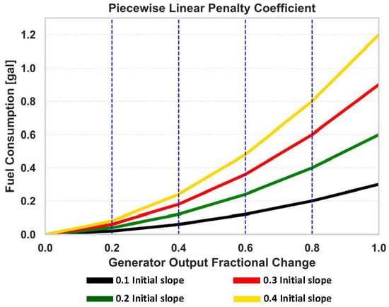
Figure 5.
Fuel consumption plots for piecewise linear penalty profiles with varying initial slopes.
Our model appears in its entirety in Appendix A, which is followed by a table containing our parameter values.
4. Results and Analysis
We now exercise our optimization model on various scenarios. We first study the impact of including an ESS in our microgrid architecture by solving the model with and without an ESS; then, we quantify the impact that various penalty terms have on the microgrid’s fuel consumption and the optimal generator and ESS usage.
We implement our model using Python’s Pyomo package and solve it using the IBM ILOG CPLEX Interactive Optimizer 12.10.0.0 on a computer with 16 GB RAM and a 2.60 Ghertz (Hz) CPU [42]. The instances described in this section contain approximately 414–9501 constraints and 221–5761 decision variables, of which 60–2016 are binary. These instances solve to a 0–1% optimality gap in approximately 1–20 s.
We consider demand data obtained during the summer months from a US FOB located in Afghanistan and collected by the Army Logistics Innovation Agency (LIA) during the Contingency Base–Demand Data Collection (CB-DDC) project. Figure 6 depicts the power demand profile in a 48 h period, which we implement in the optimization model.
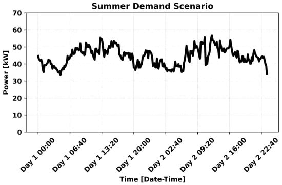
Figure 6.
US FOB power demand scenario over a 48 h time frame during the summer season.
4.1. Linear Penalty
We first consider a linear penalty term with coefficients of 0.2 gallons (gal)/, 0.4 gal/, 0.6 gal/, and 0.8 gal/. Figure 7 shows the optimal power production for each of these coefficients, which is solved to a 1% optimality gap. As the figure indicates, most of the demand is satisfied by the generator. Rapid generator fluctuations decrease substantially when any of the penalties is imposed, and the decrease is larger for a higher penalty coefficient. Figure 8 shows the battery state of charge for these instances.
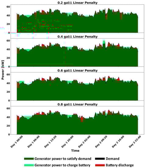
Figure 7.
Power output plot based on linear penalty coefficients imposed on the generator for the summer demand scenario.
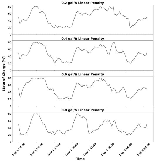
Figure 8.
Battery state of charge for the instances shown in Figure 7.
Mirroring Figure 7, Table 1 summarizes the results for each of the four penalty slope coefficients. We observe that the presence of a penalty significantly impacts the overall breakdown of power production, while the exact value of the penalty does not significantly affect this breakdown for the penalty values we consider. However, as the rightmost column indicates, an increasing penalty coefficient does increase fuel consumption when no ESS is present.

Table 1.
Optimal fuel consumption and power output with various linear penalties for the summer demand scenario.
4.2. Piecewise Linear Penalty
Finally, we consider the four piecewise linear penalty functions shown in Figure 5 and display the optimal solution for each of these four cases in Figure 9. The changes in generator and ESS optimal power production are minimal across the four piecewise linear penalty variations. Most of the demand is satisfied by the generator, as the dark green dominates the surface area of each plot. Additionally, the fluctuation in generator power output and ESS discharge rate decreases when the piecewise linear initial slope increases across the four penalties. When the generator exceeds the demand, the additional power charges the ESS for future use. Figure 10 shows the corresponding battery SOC.
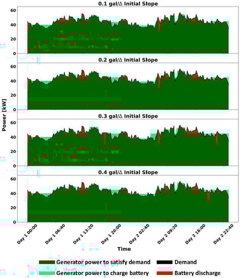
Figure 9.
Power output plot based on piecewise linear penalty coefficients imposed on the generator for the summer demand scenario.
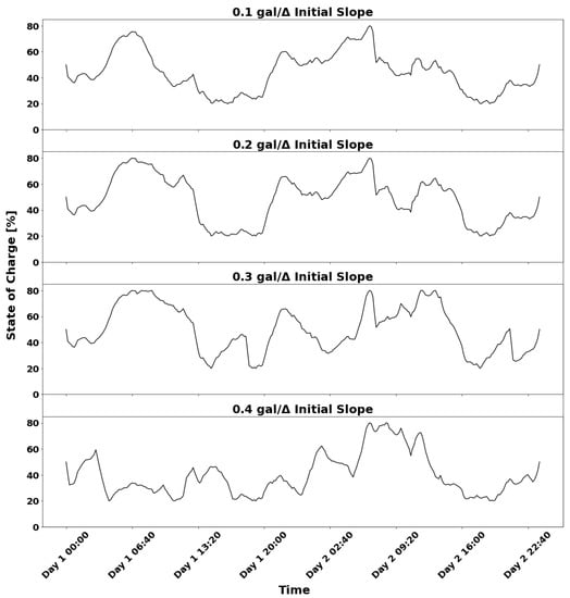
Figure 10.
Battery SOC for the instances shown in Figure 9.
Mirroring the graphical results, Table 2 depicts the corresponding numerical results for each of the different piecewise linear penalties. The results across the four piecewise linear penalties indicate that about 3% of the demand is satisfied by the ESS. The results display a consistent pattern of the generator supplying most of the demand. Again, the numerical results from the table reveal that the weight of the piecewise linear penalty coefficient is insignificant, as the generator and ESS scheduling power patterns are consistent across the four penalty variations. With no ESS present, we observe increasing fuel consumption with increased penalty coefficients, as expected.
Table 2.
Optimal fuel consumption and power output with various piecewise linear penalties for the summer demand scenario.
Figure 11 reiterates the importance of imposing a penalty on the generator. When an ESS is present but no penalty is imposed on generator fluctuations, the ESS is not utilized. This is not unexpected due to the fact that the ESS has an RTE less than 100%. While the ESS could, in principle, enable the generator to operate in a more efficient region of its production curve for a greater proportion of time, this apparently does not occur for this instance. The ESS is utilized more when a penalty is imposed on the generator, as optimization smooths out the generator power output to minimize cumulative fuel consumption.
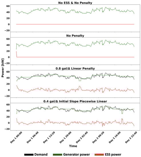
Figure 11.
Optimal power distribution over various architectures for the summer demand scenario.
4.3. Impact of ESS Round-Trip Efficiency
The generator and ESS optimal power production vary drastically between the scenario with a penalty imposed on the generator and a scenario without a penalty imposed on the generator. In general, the activity of the ESS increases significantly when a penalty is imposed on the generator. In all previous scenarios, the ESS is set to a 90% RTE, which is consistent with the research outlined in Section 2. While technological advancement may increase the ESS RTE above 90%, the price of the ESS increases rapidly as the RTE increases. This is a very important factor in microgrid design.
We now study the impact of the ESS RTE on overall fuel consumption. We consider six different ESS RTEs reflective of various ESS technologies, including future technologies achieving high efficiencies: 70%, 75%, 80%, 85%, 90%, and 95%. For each ESS RTE, we run the model using four different piecewise linear penalty functions for each of ten different 24 h demand scenarios. The cumulative fuel consumption for each of these 240 configurations appears as a circular marker in Figure 12, where ESS RTE appears on the horizontal axis and the generator penalty function is denoted by color. (For readability, we introduce a small horizontal jitter at each ESS RTE.) Solid lines indicate the average fuel consumption for each ESS RTE, broken down by penalty function. As the figure indicates, there is considerable variability among scenarios for a given ESS RTE, and the average fuel consumption decreases only modestly with increasing ESS RTE. Since a lower RTE is often cheaper to obtain, this study shows possible effects and tradeoffs that designers would have to make when selecting an ESS for their respective microgrid architecture. Our results indicate that the presence of an ESS in a microgrid is of much more importance than its exact specifications for the configuration we consider.
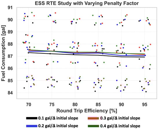
Figure 12.
Total fuel consumption for varying ESS RTE and penalty functions for ten different summer demand scenarios. Circular markers indicate individual model runs, while lines indicate average fuel consumption for each ESS RTE and penalty funtion.
5. Conclusions and Future Work
This paper formulates an MILP optimization model that prescribes optimal generator and ESS usage to minimize fuel consumption while satisfying demand. A novel feature of this model is that it includes a penalty on generator output fluctuations. This penalty represents additional fuel that is consumed when the generator’s output varies over time, and it has not been modeled in prior research. The inputs to the optimization model include a power demand scenario as well as the relevant characteristics of the generator, ESS, and penalty function.
We also exercise the MILP on a case study derived from actual FOB demand data. Our results indicate that an ESS is critical to achieving a smooth generator operating profile. When a penalty term is included in the objective function, we observe much smoother generator output profiles, with peak loads satisfied by the ESS and excess generator power used to charge the ESS during periods of low demand. This results in modest immediate fuel savings and can be expected to lengthen the operational lifetime of the generator, which is an important consideration in practice. We observe only minimal changes in our optimal solutions as we vary the magnitude of the penalty term, indicating that the presence of a penalty term is more important than its exact magnitude for the values we consider.
Future Work
While our MILP provides important insights on the impact of the penalty term on the optimal generator output profile and the resulting fuel consumption, it is not appropriate for implementation in a microgrid. The primary reason for this is that the MILP requires a complete demand profile as an input; it is thus “omniscient” and not suitable for real-time operation, where future demands are unknown. Thus, a natural next step for future research is to develop a real-time controller that attempts to replicate the smooth operating profiles observed in our optimal solutions. Our results indicate that the optimal load profiles are not sensitive to the exact form or magnitude of the penalty function. The implication of this is that if researchers can develop a real-time controller that produces load profiles similar to those obtained in our solutions, that controller can be expected to perform well in a variety of settings.
Our model excursions consider a simple microgrid architecture and demand data based on a US FOB in the Middle East. It is critical to explore multiple microgrid architectures when varying locations have different resources and technologies available. An appropriate next step is to alter the microgrid architectures by implementing different generators of varying sizes or even modifying the discharging and charging rates of the ESS as well as exploring additional demand scenarios.
With the initial exploration of generator penalty terms using a simple microgrid optimization model, this paper shows that a simple penalty term imposed on the generator has a significant influence on the optimal solution and overall fuel consumption. Due to the lack of empirical real-world data, our penalty terms are only notional. Further studies in the field are needed to examine the effect of time-varying loads on generator efficiency. These studies will lead to more realistic penalty terms that can optimally distribute power between the generator and ESS more accurately.
Author Contributions
Conceptualization, E.C., A.K. and G.O.; methodology, E.C., A.K. and G.O.; software, J.W.L. and E.C.; validation, J.W.L., E.C., A.K. and G.O.; formal analysis, E.C., A.K. and J.W.L.; investigation, J.W.L.; resources, E.C., A.K.; data curation, J.W.L., E.C. and A.K.; writing—original draft preparation, J.W.L.; writing—review and editing, J.W.L., E.C., A.K. and G.O.; visualization, J.W.L.; supervision, E.C., G.O. and A.K.; project administration, A.K. and E.C.; funding acquisition, A.K. All authors have read and agreed to the published version of the manuscript.
Funding
This research was funded by the Energy System Technology Evaluation Program and by the Office of Naval Research.
Institutional Review Board Statement
Not applicable.
Informed Consent Statement
Not applicable.
Data Availability Statement
Source data and code are available upon request from the authors.
Acknowledgments
This research is partially supported by the Naval Postgraduate School. Any opinions or findings of this work are the responsibility of the authors, and do not necessarily reflect the views of the sponsors or collaborators.
Conflicts of Interest
The authors declare no conflict of interest.
Appendix A. FOB Model with Linear Piecewise Penalty
Sets and Indices:
| Time periods | |
| Generator operating region (for linearization purposes) | |
| Generator fractional change regions (for linearization purposes) |
Parameters:
| Generator base fuel consumption slope (gal/kW) | |
| Generator base fuel consumption intercept (gal) | |
| Load that is demanded in time step t (kW) | |
| Start of fractional change region i (kW) | |
| End of fractional change region i (kW) | |
| Lower boundary of penalty region h () | |
| Upper boundary of penalty region h () | |
| Slope of penalty function in region h (gal/) | |
| Intercept of penalty function in region h (gal) | |
| Time step (hours) | |
| Battery capacity (kWh) | |
| Discharge efficiency of battery | |
| Charge efficiency of battery | |
| Maximum battery rate of charge (kW) | |
| Maximum battery rate of discharge (kW) | |
| Minimum generator load (kW) | |
| Maximum generator load (kW) | |
| Minimum battery state of charge (%) | |
| Maximum battery state of charge (%) |
Decision Variables:
| Continuous | Generator power flow in time step t (kW) | |
| Continuous | Power flow used to charge battery in time step t (kW) | |
| Continuous | Power flow out of battery in time step t (kW) | |
| Continuous | Battery state of charge in time step t (%) | |
| Continuous | Absolute difference in generator power flow between time step and t (kW) | |
| Binary | 1 if in region i in time step t and 0 otherwise | |
| Continuous | Auxiliary variable used for linearization: (kW) | |
| Continuous | Fractional [0-1] change in generator power flow between time step and t | |
| Binary | 1 if in region h in time step t and 0 otherwise | |
| Continuous | Auxiliary variable used for linearization: |
Objective Function:
Constraints:
Table A1.
Parameter Values.
Table A1.
Parameter Values.
| Parameter | Value |
|---|---|
| 0.0113 | |
| 0.0933 | |
| h | |
| 25 kWh | |
| % | |
| % | |
| 20 kW | |
| 20 kW | |
| 15 kW | |
| 60 kW | |
| 20% | |
| 80% |
References
- Schwartz, M.; Blakely, K.; O’Rourke, R. Department of Defense Energy initiatives: Background and issues for Congress; CRS Report R42558; Congressional Research Service: Washington, DC, USA, 2012. [Google Scholar]
- Office of the Assistant Secretary of Defense for Energy, Installations, and Environment. New Operational Energy Strategy Released by the Department. 2018. Available online: https://www.acq.osd.mil/eie/OE/OE%20Strategy%20Page.html (accessed on 6 March 2021).
- Katiraei, F.; Iravani, M.R.; Lehn, P.W. Micro-grid autonomous operation during and subsequent to islanding process. IEEE Trans. Power Deliv. 2005, 20, 248–257. [Google Scholar] [CrossRef]
- Morstyn, T.; Hredzak, B.; Aguilera, R.P.; Agelidis, V.G. Model predictive control for distributed microgrid battery energy storage systems. IEEE Trans. Control Syst. Technol. 2018, 26, 1107–1114. [Google Scholar] [CrossRef]
- Hartono, B.S.; Budiyanto, Y.; Setiabudy, R. Review of microgrid technology. In Proceedings of the 2013 International Conference on QiR, Yogyakarta, Indonesia, 25–28 June 2013; pp. 127–132. [Google Scholar] [CrossRef]
- Ton, D.; Reilly, J. Microgrid controller initiatives: An overview of RD by the U.S. Department of Energy. IEEE Power Energy Mag. 2017, 15, 24–31. [Google Scholar] [CrossRef]
- Craparo, E.; Sprague, J. Integrated supply- and demand-side energy management for expeditionary environmental control. Appl. Energy 2019, 233–234, 352–366. [Google Scholar] [CrossRef]
- Sprague, J.G. Optimal Scheduling of Time-Shiftable Electric Loads in Expeditionary Power Grids. Master’s Thesis, Naval Postgraduate School, Monterey, CA, USA, 2015. [Google Scholar]
- Garcia, K. Optimization of Microgrids at Military Remote Base Camps. Master’s Thesis, Naval Postgraduate School, Monterey, CA, USA, 2017. [Google Scholar]
- Kiser, E. The Impact of Technologies and Missions on Contingency Base Fuel Consumption. Master’s Thesis, Naval Postgraduate School, Monterey, CA, USA, 2018. [Google Scholar]
- Anglani, N.; Oriti, G.; Colombini, M. Optimized energy management system to reduce fuel consumption in remote military microgrids. IEEE Trans. Ind. Appl. 2017, 53, 5777–5785. [Google Scholar] [CrossRef]
- Cummins Inc. Advanced Medium Mobile Power Sources (AMMPS). 2017. Available online: http://power.cummins.com/system/files/literature/brochures/Advanced_Medium_Mobile_Power_Sources_Brochure.pdf (accessed on 8 October 2022).
- Di Cairano, S.; Liang, W.; Kolmanovsky, I.V.; Kuang, M.L.; Phillips, A.M. Power Smoothing Energy Management and Its Application to a Series Hybrid Powertrain. IEEE Trans. Control Syst. Technol. 2013, 21, 2091–2103. [Google Scholar] [CrossRef]
- Ahmed, M.; Vahidnia, A.; Meegahapola, L.; Datta, M. Small signal stability analysis of a hybrid AC/DC microgrid with static and dynamic loads. In Proceedings of the 2017 Australasian Universities Power Engineering Conference (AUPEC), Melbourne, Australia, 19–22 November 2017; pp. 1–6. [Google Scholar] [CrossRef]
- Fakhrazari, A.; Vakilzadian, H.; Choobineh, F.F. Optimal energy scheduling for a smart entity. IEEE Trans. Smart Grid 2014, 5, 2919–2928. [Google Scholar] [CrossRef]
- Siritoglou, P.; Oriti, G.; Van Bossuyt, D.L. Distributed Energy-Resource Design Method to Improve Energy Security in Critical Facilities. Energies 2021, 14, 2773. [Google Scholar] [CrossRef]
- Reich, D.; Oriti, G. Rightsizing the Design of a Hybrid Microgrid. Energies 2021, 14, 4273. [Google Scholar] [CrossRef]
- Gamarra, C.; Guerrero, J.M. Computational optimization techniques applied to microgrids planning: A review. Renew. Sustain. Energy Rev. 2015, 48, 413–424. [Google Scholar] [CrossRef]
- Kazem, H.A.; Khatib, T. A novel numerical algorithm for optimal sizing of a photovoltaic/wind/diesel generator/battery microgrid using loss of load probability index. Int. J. Photoenergy 2013, 2013, 718596. [Google Scholar] [CrossRef]
- Katiraei, F.; Abbey, C. Diesel plant sizing and performance analysis of a remote wind-diesel microgrid. In Proceedings of the 2007 IEEE Power Engineering Society General Meeting, Tampa, FL, USA, 24–28 June 2007; pp. 1–8. [Google Scholar] [CrossRef]
- Ulmer, N. Optimizing Microgrid Architecture on Department of Defense Installations. Master’s Thesis, Naval Postgraduate School, Monterey, CA, USA, 2014. [Google Scholar]
- Bahramirad, S.; Reder, W.; Khodaei, A. Reliability-constrained optimal sizing of energy storage system in a microgrid. IEEE Trans. Smart Grid 2012, 3, 2056–2062. [Google Scholar] [CrossRef]
- Chen, S.X.; Gooi, H.B.; Wang, M.Q. Sizing of energy storage for microgrids. IEEE Trans. Smart Grid 2012, 3, 142–151. [Google Scholar] [CrossRef]
- Moradi, H.; De Groff, D.; Abtahi, A. Optimal energy scheduling of a stand-alone multi-sourced microgrid considering environmental aspects. In Proceedings of the 2017 IEEE Power Energy Society Innovative Smart Grid Technologies Conference (ISGT), Washington, DC, USA, 23–26 April 2017; pp. 1–5. [Google Scholar] [CrossRef]
- Liu, J.; Huang, X.; Zuyi, L. Multi-time scale optimal power flow strategy for medium-voltage DC power grid considering different operation modes. J. Mod. Power Syst. Clean Energy 2020, 8, 46–54. [Google Scholar] [CrossRef]
- Craparo, E.; Karatas, M.; Singham, D.I. A robust optimization approach to hybrid microgrid operation using ensemble weather forecasts. Appl. Energy 2017, 201, 135–147. [Google Scholar] [CrossRef]
- Bouaicha, H.; Craparo, E.; Dallagi, H.; Nejim, S. Dynamic optimal management of a hybrid microgrid based on weather forecasts. Turk. J. Electr. Eng. Comput. Sci. 2020, 28, 2060–2076. [Google Scholar] [CrossRef]
- del Valle, Y.; Venayagamoorthy, G.K.; Mohagheghi, S.; Hernandez, J.; Harley, R.G. Particle Swarm Optimization: Basic concepts, variants and applications in power systems. IEEE Trans. Evol. Comput. 2008, 12, 171–195. [Google Scholar] [CrossRef]
- Li, H.; Eseye, A.T.; Zhang, J.; Zheng, D. Optimal energy management for industrial microgrids with high-penetration renewables. Prot. Control Mod. Power Syst. 2017, 2, 12. [Google Scholar] [CrossRef]
- Kim, R.K.; Glick, M.B.; Olson, K.R.; Kim, Y.S. MILP-PSO Combined Optimization Algorithm for an Islanded Microgrid Scheduling with Detailed Battery ESS Efficiency Model and Policy Considerations. Energies 2020, 13, 1898. [Google Scholar] [CrossRef]
- Das, A.; Ni, Z. A Computationally Efficient Optimization Approach for Battery Systems in Islanded Microgrid. IEEE Trans. Smart Grid 2018, 9, 6489–6499. [Google Scholar] [CrossRef]
- Zhu, D.; Broadwater, R.; Tam, K.S.; Seguin, R.; Asgeirsson, H. Impact of DG placement on reliability and efficiency with time-varying loads. IEEE Trans. Power Syst. 2006, 21, 419–427. [Google Scholar] [CrossRef]
- Hernandez-Aramburo, C.A.; Green, T.C.; Mugniot, N. Fuel consumption minimization of a microgrid. IEEE Trans. Ind. Appl. 2005, 41, 673–681. [Google Scholar] [CrossRef]
- Bhandari, Y.; Chalise, S.; Sternhagen, J.; Tonkoski, R. Reducing fuel consumption in microgrids using PV, batteries, and generator cycling. In Proceedings of the IEEE International Conference on Electro-Information Technology, EIT 2013, Rapid City, SD, USA, 9–11 May 2013; pp. 1–4. [Google Scholar] [CrossRef]
- Xiao, Z.X.; Guan, Y.Z.; Fang, H.W.; Terriche, Y.; Guerrero, J.M. Dynamic and Steady-State Power-Sharing Control of High-Efficiency DC Shipboard Microgrid Supplied by Diesel Generators. IEEE Syst. J. 2022, 16, 4595–4606. [Google Scholar] [CrossRef]
- Kapetanović, M.; Núñez, A.; van Oort, N.; Goverde, R.M. Reducing fuel consumption and related emissions through optimal sizing of energy storage systems for diesel-electric trains. Appl. Energy 2021, 294, 117018. [Google Scholar] [CrossRef]
- Downs, J.; Marinelli, A.; Fowler, K.; Duncan, J.; Hamm, K.; Choi, E.; McCabe, K.; Boyd, P. Contingency Base Demand Data Collection for Buildings and Facilities; Technical Report PNNL-26065; Pacific Northwest National Laboratory: Richland, WA, USA, 2016. [Google Scholar]
- Singleton, B.; (US Army Base Camp Integration Lab, Fort Devens, MA, USA). Email Exchanges and Site Visit, Personal Communication, 2017.
- Li, K.; Tseng, K.J. Energy efficiency of lithium-ion battery used as energy storage devices in micro-grid. In Proceedings of the IECON 2015—41st Annual Conference of the IEEE Industrial Electronics Society, Yokohama, Japan, 9–12 November 2015; pp. 005235–005240. [Google Scholar] [CrossRef]
- Moseley, P.T.; Garche, J. Chapter 4: Applications and markets for grid-connected storage systems. In Electrochemical Energy Storage for Renewable Sources and Grid Balancing; Moseley, P.T., Garche, J., Eds.; Elsevier: Amsterdam, The Netherlands, 2015; pp. 440–443. [Google Scholar] [CrossRef]
- Majima, M.; Ujiie, S.; Yagasaki, E.; Koyama, K.; Inazawa, S. Development of long life lithium ion battery for power storage. J. Power Sources 2001, 101, 53–59. [Google Scholar] [CrossRef]
- International Business Machines Corporation (IBM). IBM ILOG CPLEX Optimization Studio (CPLEX). 2009. Available online: https://www.ibm.com/products/ilog-cplex-optimization-studio (accessed on 17 October 2022).


Publisher’s Note: MDPI stays neutral with regard to jurisdictional claims in published maps and institutional affiliations. |
© 2022 by the authors. Licensee MDPI, Basel, Switzerland. This article is an open access article distributed under the terms and conditions of the Creative Commons Attribution (CC BY) license (https://creativecommons.org/licenses/by/4.0/).