Abstract
The Paris Climate Agreement and the 2030 Agenda for Sustainable Development Goals declared by the United Nations set high expectations for the countries of the world to reduce their greenhouse gas (GHG) emissions and to be sustainable. In order to judge the effectiveness of strategies, the evolution of carbon dioxide, methane, and nitrous oxide emissions in countries around the world has been explored based on statistical analysis of time-series data between 1990 and 2018. The empirical distributions of the variables were determined by the Kaplan–Meier method, and improvement-related utility functions have been defined based on the European Green Deal target for 2030 that aims to decrease at least 55% of GHG emissions compared to the 1990 levels. This study aims to analyze the energy transition trends at the country and sectoral levels and underline them with literature-based evidence. The transition trajectories of the countries are studied based on the percentile-based time-series analysis of the emission data. We also study the evolution of the sector-wise distributions of the emissions to assess how the development strategies of the countries contributed to climate change mitigation. Furthermore, the countries’ location on their transition trajectories is determined based on their individual Kuznets curve. Runs and Leybourne–McCabe statistical tests are also evaluated to study how systematic the changes are. Based on the proposed analysis, the main drivers of climate mitigation and evaluation and their effectiveness were identified and characterized, forming the basis for planning sectoral tasks in the coming years. The case study goes through the analysis of two counties, Sweden and Qatar. Sweden reduced their emission per capita almost by 40% since 1990, while Qatar increased their emission by 20%. Moreover, the defined improvement-related variables can highlight the highest increase and decrease in different aspects. The highest increase was reached by Equatorial Guinea, and the most significant decrease was made by Luxembourg. The integration of sustainable development goals, carbon capture, carbon credits and carbon offsets into the databases establishes a better understanding of the sectoral challenges of energy transition and strategy planning, which can be adapted to the proposed method.
1. Introduction
Greenhouse gas (GHG) emission is considered the most significant anthropogenic driving force of climate change [1]. In 2020, fossil fuels were taking around 80% of primary energy consumption [2]. Due to this high fossil fuel consumption percentage, the reserve-to-production (R/P) ratio of fossil fuels is significantly decreasing. R/P defines the availability of fossil fuels (such as oil, natural gas, and coal reserves) in years. However, primary energy consumption decreased by 4.5% compared to 2019, from which oil consumption dropped 9.5%, natural gas dropped 3.1%, and coal dropped 4.1%; still, the total world resources in oil last only for 50 years of current production. Regions with the lowest reserves are Europe with 10.4 years and the Asia Pacific with 16.6 years [2].
This recognition stimulated international agreements to mitigate the accelerated climate change processes and raised the attention that countries’ transition paths toward climate neutrality need to be continually monitored. In September 2015, the 2030 Agenda for Sustainable Development adopted by the United Nations declared 17 development goals, from which the 13th is the “Take urgent action to combat climate and its impacts” [3]. It addressing decreasing greenhouse gas emissions, considers climate finance, and fosters adaptation strategies. In parallel, in December 2015, the Paris Agreement was signed to support countries dealing with climate change impact and accelerate global cooperative climate actions. The primary target of the agreement is to keep the global average temperature well below 2 °C above pre-industrial levels and then further limit the increase to 1.5 °C [4]. Strategic planning should consider changes in dynamics, such as the effects of COVID-19 on energy conversion [5]. Defossilization and electrification are of paramount importance for the entire energy system [6], which are scenarios that are compatible with the Paris Agreement [7]. The sectoral exploration of the structural changes brought about by changes in the quantity and type of energy services is also called for in the 2030 Agenda for Sustainable Development Goals [8]. This may require down-sizing the global energy system as low-carbon supply-side transformation strategies [9]. Another driving force is the European Green Agreement, which sets a 55% reduction in carbon emissions in the same way as the SDG framework by 2030 and carbon neutrality in EU countries by 2050 [10]. These new policies are expectations for energy transition and a green economy that countries must meet.
In order to meet the requirements of the agreements, member states have to transition their current environmental strategies toward social, economic, and environmental sustainability [11]. The objective of this study is to support decision-making and policy formulation to meet the requirements by systematically exploring the components of the dynamics of raw GHG emission values by conducting country and sector-wise analyses of energy transition paths based on the time series of percentiles and presenting them relative to current studies. This study further aims is to enrich the framework for the energy transition to global low-carbon energy by identifying the time series of related sectors, scoring the distance from the Green Deal target in 166 countries, and integrating economic drivers to provide a higher level of sustainability satisfaction. However, it is essential to highlight that global GHG inventories generally neglect efforts of carbon offsetting [12], the impacts of implemented carbon capture technologies [13] or even a traceable account of carbon credits [14], which can significantly affect those dynamics. The proposed analyses may reveal transparent information that supports the understanding of spatial and temporal details of the energy sectors and their synergies required for cross-sectoral decarbonization models [15].
Recent studies have attempted to estimate whether countries can reach the Green Deal targets or not. Dolge et al. have estimated the progress toward implementing Green Deal targets and identified the drivers of GHG emission changes in the European Union using Kaya identity and Log Mean Divisia Index (LMDI) decomposition from data between 2010 and 2019 [16]. Furthermore, Hainsch et al. have developed a three-dimensional (policy, technology, society) scenario methodology used for the four openENTRANCE pathways to generate and evaluate four different energy transition pathways, which showed that the European energy transition success is highly dependent on the three dimensions [17]. Furthermore, regional emission pathways have been analyzed considering cost-effectiveness, equality, and grandfathering principles to identify whether regions will reach carbon neutrality before 2070 to meet the 2 °C climate targets [18]. The phenomena of eco-innovation facilitate transitions toward carbon neutrality, green consumption, and production by developing products and processes based on economical and environmentally efficient concepts, applications, and technologies [19].
The GHG emissions of the countries have been investigated from diverse aspects with data-driven techniques. The vulnerability to negative effects of climate change was investigated in the case of the 36 highest emitting countries [20]. The relations between immigration and emission also produced significant results [21]. The effect of indirect emission [22], COVID-19 [23], animal agriculture [24], energy innovation [25], and the effects of foreign direct investments, governance, democracy, renewable energy use, and economic growth on carbon dioxide emission [26] were also investigated. Based on the measures of GHG emissions, financial and economic analysis has been carried out for Montenegro. However, it faces limitations due to different degrees of data reliability [27]. The relationship between carbon emission and economic growth at the world level and three income levels (upper middle income, lower middle income, and high income) has been analyzed by Wang et al. from 1990 to 2014 under the background of the energy transition. Furthermore, Gencer et al. presented a system-scale energy analysis tool that assesses system-level GHG emissions of the energy system and analyzes life cycle emissions of the energy transition [28]. In terms of environmental communication and monitoring, visuals can be powerful tools, as they have the ability to present and summarize large amounts of complex information [29].
The continuous monitoring of countries’ performance regarding their GHG emissions is commonly agreed upon; however, comprehensive and comparable analysis of the trends in countries’ performances based on percentiles has not been emphasized. The percentile-based analysis of the time-series emissions data enables easy comparison of how the distribution of emissions is changing and where countries are located compared to each other overall and sector-wise. Furthermore, climate change-related utility functions can be defined. The primary objective of this paper is to provide an overview of the efficiency of countries’ energy transition strategies and their trends in total and sectoral emission based on the time series of percentiles. The percentile-based analysis of sectoral emissions supports the identification of the significance of the sectors and their contribution to the total emission, which is needed due to the significance of every sector in an economy, and for reducing emission, phase-wise energy management in each sector is needed [30]. The analysis of greenhouse gas emissions by sectors is evident for countries to detect focus areas that need to be addressed to reach climate neutrality. The evolution of greenhouse gas concentrations such as carbon dioxide (), methane (), and nitrous oxide () emissions are explored based on time-series data between 1990 and 2018 [31]. The equivalent is calculated for the gases for a comparable overview. The majority of greenhouse gases arise from economic activity, which results in an inevitable effect on environmental defects such as heat waves, hurricanes, droughts, wildfires, and environmental-related diseases [32].
It is necessary to understand the association between environmental degradation and the economy in a country, so based on the information on its energy transition path, more adequate policy mitigation initiatives can be created [33]. Therefore, to gain better insight into counties’ location of their transition trajectories, the theory of the environmental Kuznets curve (EKC) is used. The environmental Kuznets curve hypothesis assumes a relationship between economic development and the environment, which results in an inverted U-shape curve [34]. The Kuznets curve declares that during the development phase of a country, the environmental pollution increases, but when a country reaches a particular development phase with rising income, a turning point can be observed, and the pollution decreases.
Comprehensive models and methods utilizing temporal, spatial, and sectoral aspects should be considered by policymakers to better understand energy transition and form policies that support the transition toward carbon neutrality [17]. The energy transition is characterized by increasing cross-sectoral synergies, open access, and growing coverage of better time series; nevertheless, the coupling of tools and sectoral challenges poses further research [15]. Therefore, this research focuses on developing an analytical and visualization methodology suitable for mapping sectors’ contributions. This paper detects global, country-wise, and sectoral emissions production trends through the percentile-based analysis and time-series mapping of the empirical distribution of emission data of world countries. The proposed analysis helps to better understand the global patterns of different energy transition strategies. This study evaluates the relationships between the time series of GDP per capita and the total emission ( equivalent) of world countries, discusses the sectoral contribution to climate change, and positions the results relative to recent studies. Therefore, the main contributions of the work are the following:
- A global, detailed overview of current GHG emission distribution change is provided and presented relative to recent research.
- A novel analytical technique is introduced, the percentile plot, to compare contributions to climate change.
- The sector breakdown of the data is considered to identify the driving sectors of climate change that need to be addressed.
- Improvement-related variables are defined subject to the European Green Deal-based utility function.
- The transition trajectories of the countries are determined by environmental Kuznets curves.
We believe that the proposed aspects bring value to greenhouse gas emissions monitoring and prediction research, and the proposed new type of emission data representation and analysis helps to gain a deeper understanding of the differences in countries’ energy transition paths.
In the following, the article is structured as follows, Section provides a detailed description of the time-series data. Section 2 introduces the proposed methodology and the data sources used and integrated for the analysis. The analysis of the results is discussed in Section 3.1 and presented in the context of current research.
2. Methodology
In this section, the proposed methodology is presented. The structure of the methodology is shown in Figure 1. The emission data are analyzed from the country and sectoral aspects, indicating sectors and subsectors in the figure. The time-series emission data used for the analysis are also structured accordingly. Carbon dioxide, methane, nitrous oxide, and fluorinated gases were considered during the analysis, of which the equivalent is calculated to obtain a better comparison.
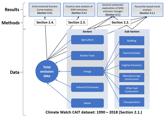
Figure 1.
The sectorial breakdown of the GHG emissions and its application for the exploration of GHG emission patterns.
equivalent measures the Global Warming Potential (GWP). GWP allows comparing the global warming impact of greenhouse gases regarding their ability to absorb energy and stay in the atmosphere. It measures how much energy the emissions of 1 ton of a gas will absorb over a given period of time relative to the emissions of 1 ton of carbon dioxide (); therefore, GWP-weighted emissions are in a million metric tons of equivalent [35]. The GWP value of is 1, which is used as the reference. It has remained in the climate system for thousands of years. Carbon dioxide is released into the atmosphere when burning fossil fuels (oil, natural gas, and coal), solid waste, trees, and other biological materials; chemical reactions (e.g., cement manufacture) release . The GWP value of is 25 over 100 years and lasts about a decade but absorbs more energy. Methane is emitted during oil, natural gas, coal production and transport, agricultural activities, livestock, and organic waste decay in municipal solid waste landfills. Meanwhile, the GWP value of is 298 and has remained in the atmosphere for more than 100 years. Nitrous oxide is emitted during agricultural, land use, industrial activities, the combustion of fossil fuels and solid waste, and wastewater treatment. In 2019, the United States measured 6.558 million metric tons of -equivalent, from which 74.1% were emitted during fossil fuel combustion, and forests and other lands absorbed only 12.4% of total emissions [35].
During the analyses, we considered the time series of GHG gases mentioned above and analyzed them according to the sectoral dimensions and world countries. The background of trends and the given results are compared with recent research findings.
Information about the data source and its integration are introduced in Section 2.1. The method of analyzing the time series of the percentiles and the generation of improvement-related variables are described in Section 2.2, while the Kuznets analysis is presented in Section 2.4. The detailed results are presented in the subsections of Section 3.1, which are grouped according to methodological subsections, as structurally summarized in Figure 1.
2.1. Data Sources and Integration
The time-series data of greenhouse gas emissions are based on the CAIT dataset included on the Climate Watch website [31]. The dataset includes all GHGs and provides a sectoral breakdown, which is shown in Figure 1.
The dataset includes historical data from 1990 until 2018. The emissions production (referred to as emissions) per capita values are calculated based on the population data taken from the World Bank Database, from where the GDP data were also downloaded [36]. Per capita emissions were used, since it considers the size of countries’ activities and can provide a better comparison between countries and their trends [37].
The available dataset is structured into a multidimensional array (tensor), , where the elements of the four-dimensional array represent the emissions/capita values, where the i index represents the type of gas (carbon dioxide, and equivalents of methane, nitrous oxide and fluorinated gasses), the j index represents the sectors, which can be seen Figure 1, k stands for the index of the year, and l stands for the index of the country, , as countries with a population of less than 300.000 were excluded from the study. This representation is beneficial as the multidimensional array can be easily aggregated; e.g., the shows how much GHG an average person has emitted in the k-th year in the l-th country.
2.2. Analysis of the Time Series of the Percentiles and Improvement Related Variables
As we are interested in extracting compact and easily interpretable information from the time-series analysis of the GHG data, we first study how the emissions’ distribution is changing. For this purpose, the empirical cumulative distribution functions (ECDF) of the GHGs have been determined for every year, every sector, and every gas type. The function shows the probability that the GHG emission in a randomly selected country is higher than a particular value:
The empirical distribution functions are determined by Kaplan–Meier estimation, which can be calculated as [38]:
where represents the number of countries that have the same GHG emission as , while stands for the number of countries that have not been considered between and GHG emission values.
The significant advantage of the calculation of empirical distributions is that the percentiles of the given sample can be easily determined from the distribution function. The resulted percentiles are also stored in a four-dimensional array. The percentile values can be easily interpreted; e.g., represents that the emission per capita value of the i-th gas in the j-th sector in year k is the highest among the countries in the category defined by the i-th gas and the j-th sector. Similarly, stands for the smallest emission. The value for probability 0.5 corresponds to the median, while the 3rd quartile corresponds to 0.75, and the 1st quartile corresponds to 0.25. Let us consider an example empirical distribution function derived from the dataset {1, 4, 6, 7, 8} in Figure 2. For that case, the maximum value is , the third quartile is , the median is , the first quartile is , and finally, the minimum is .
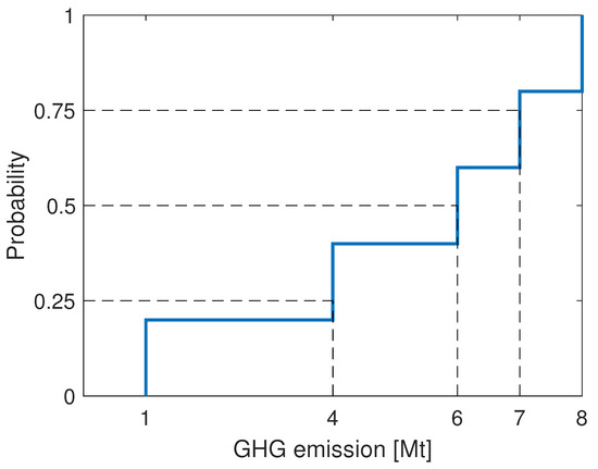
Figure 2.
The determination of the percentiles based on an example empirical distribution function. The maximum value is , the third quartile is , the median is , the first quartile is , and finally, the minimum is .
The key idea of the proposed method is that the visualization of the time series of percentiles (especially the minimum, the maximum, the median, and the lower and upper quartiles) highlights how the distribution of the emissions is changing. The main benefit of the resulting graph is that by showing the time series of the percentiles of a given country, the transition path of the country can be easily depicted, and the visualization shows how successful the transformation is compared to other countries.
Regarding the comparison of transformation, we can also study the distribution of the improvement ratios related to the European Green Deal targets for 2030. The European Green Deal member states agreed to reduce their GHG emission by at least 55% compared to 1990. The distribution of the improvement ratio is calculated as
This measure can highlight on which level the emission was changed. However, the relative change to the benchmark level is interesting for the European Green Deal. In that case, the percentage change to the 1990 level can be defined as:
Although the European Green Deal was only established between the European Union member states, the target to decrease the GHG emission of countries is an overall desire. Therefore, the Green Deal-based utility function can be extended to the world’s countries. With this tool, the state of the reduction process can be examined over the years. This comparison is a first step to identifying an initial rank of countries based on their GHG reduction percent and seeing how much countries have decreased their emission compared to the levels in 1990. Countries that have already fulfilled this deal (under the target level) can be identified based on the last year of the dataset (2018). However, it must be noted that the origin of the decrease in emission must be determined to gain a complex view of the connection between countries’ economic and environmental performances. By comparing to other years, it is possible to forecast based on the trend of change which country can perform it for 2030.
The difference in emission values between two years defines another measure and gives the analysis a new perspective.
This idea can define another type of ranking, describing how the countries changed their emission over the years. A top list of the most reduced or increased countries can be made. Based on the changes in a period, the environmental pollution of a given country can be determined more precisely by analyzing the direction of the change and the achieved emission level.
2.3. Characterization of the Time Series of GHG Emissions
This paper aims to enrich the toolset of the goal-oriented analysis of the time series of the integrated GHG emission data. The first step of the proposed method is to determine how systematic is the trend of a given emission. The runs test is a statistical method to evaluate the randomness of a time series [39]. The test checks whether a pattern, called a run, is formed in the time series; e.g., significant consecutive points below the average suggest that the time series is not random [40].
Parallel with the runs test, the stationarity of the time series can also be examined to check whether the time series maintain their statistical properties over time.
Stationary time series in GHG emission change can also imply systematic transition of the GHG emission. The stationarity properties of the time series were checked by the Leybourne–McCabe test [41]. The next section details how these measures can be applied to evaluate the transitions of the GHG emissions.
2.4. Kuznets Analysis
The environmental Kuznets curve (EKC) describes a hypothetical relationship between a country’s environmental pollution and a country’s income [42]. It is informative in itself for a time series that the presence or absence of the EKC hypothesis can be observed. The EKC model can generally be described as follows [43]:
where C denotes GHG emission, Y stands for economic growth, D refers to context-specific explanatory variables, i represents cross-sections, t denotes the time series, is a constant, refers to coefficients, and shows the standard error. In this abstraction, seven types of EKC functions can be identified according to the ratio of terms, such as inverse U-shape, U-shape, N-shape, inverted N-shape, linear increase, linear decrease, and no association. The EKC analysis can be extended to other indicators describing the state of the environment, such as the ecological footprint [44] and impact of urbanization [45]. The inverse U-shaped EKC function can be divided into three stages [46]: pre-industrial, industrial, and post-industrial economies, as can be seen in Figure 3. As in the case of Kenya, the inverted U-shaped curve has been identified and used to examine the relationship between energy consumption and renewable consumption and emissions [47]. In the pre-industrial economies phase, a country begins to develop and increases pollutant emissions. The next phase is the industrial economy, when the country reaches a level of development and can afford to allocate resources to green solutions. In that case, the function reaches a turning point so that emissions decrease while GDP continues to grow. Finally, the higher levels of development result in a shift toward information-intensive industries, services using technological alignments, higher environmental expenditures, and increased awareness and enforcement. It results in a steady reduction in emissions, GDP grows, and this phase is called the post-industrial economics section [48]. The aim is to shift economic stability, well-being, and environmental protection. In this study, the empirical environmental Kuznets curve of the world and different countries is plotted over the years to determine their position on their transition trajectories. Based on the functions, the countries’ development levels can be determined. Moreover, a penalty system could also be established, penalizing more if a developed country emits many GHGs. Unfortunately, the theoretical Kuznets hypotheses cannot be accepted in every country; however, in most cases, there is support for the EKC hypothesis, as it was tested by Churchill et al. for OECD countries [49]. Moreover, several studies have already investigated if the EKC exists in various countries even in different time intervals [50]. However, this study highlights how the Kuznets curves can enrich understanding the reasons for GHG emissions and the position in industrial phases in different countries. A future research direction is to forecast when countries or the world will reach the tipping point. Furthermore, the impacts of renewable energy (RKC) accelerate the achievement of the EKC turning point because RKC turning points occur earlier than the EKC [51].
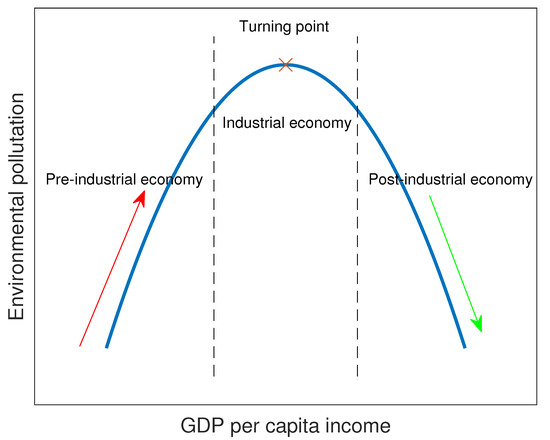
Figure 3.
The theoretical inverted U-shaped Kuznets curve (). The function has three stages: pre-industrial, industrial, and post-industrial economies. If a country moves on the Kuznets curve in the direction of the red arrow, this implies a developing country with increasing income causing increasing environmental pollution. On the contrary, moving along the green arrow implies a developed country with increasing income but decreasing emissions because they have financial effort to take care of the environment. The turning point is marked by the red X.
3. Results and Discussion
This section presents how the proposed method can be applied to analyze the GHG emission time series. The analysis of the time series with the suggested percentile-based plot is presented in Section 3.1, and the evaluation of the consistency of the sector-wise transition is discussed in Section 3.2. Then, the generation of improvement-related variables is introduced in Section 3.3. Finally, the Kuznets analysis is presented in Section 3.4.
3.1. Analysis of the Global Trends in the Time Series of the Percentiles of GHG Emissions
In order to mitigate climate change impacts, transition strategies are highly demanded in terms of how we organize our societies, institutions, and infrastructure [52]. Research and policy making must consider the overall scale of resource use and emissions and sustainable consumption corridors and their impact on climate change and well-being [53]. A rapid change in people’s attitudes and lifestyles toward sustainable consumption is required [54] to remain within planetary boundaries [55].
To fairly compare countries’ contributions to climate change, the percentile plot of total GHG emissions produced per country is shown in Figure 4. It must be noted that the analysis has been made for the world countries. Still, for better interpretability, only two countries are shown as examples during the whole paper: Sweden and Qatar. Percentile values are determined based on the emissions data of countries in each year between 1990 and 2018. The maximum, third quartile (Q3), median (Q2), first quartile (Q1), and minimum functions are indicated on the plot. Here, 25% of countries’ emissions production fall between 0 and 2.851 per capita per year, while the interquartile range (Q2–Q1) is between 2.399 and 8.019 per capita. The annual emission of countries is slowly approaching the median (4.877 per capita in 2018). In this example, two countries’ performances are represented: Qatar and Sweden. Notably, Qatar’s annual emission per capita equals the maximum since 1995, as its economy is driven by oil and natural gas reserves. In 2008, the Qatar National Vision 2030 was signed with the aim of comprehensive development in economic, social, and environmental management to become a developed country by 2030 [56]. Although the GDP per capita of Qatar significantly increased, the greenhouse gas emissions per capita are still the highest (35.89 per capita in 2018). In contrast, Sweden’s GDP is continually rising, while their GHG emissions indicate a continual decrease (from 7.991 to 4.55 per capita between 1990 and 2018). However, after the crisis in 2008, a temporary increase in emission was observed. Furthermore, after the Paris Agreement in 2015, Sweden’s emission per capita has been lower than the median. Sweden’s long-term emission target for 2045 is to have no net emissions of greenhouse gases to the atmosphere, which means an 85% decrease compared to 1990 [57].
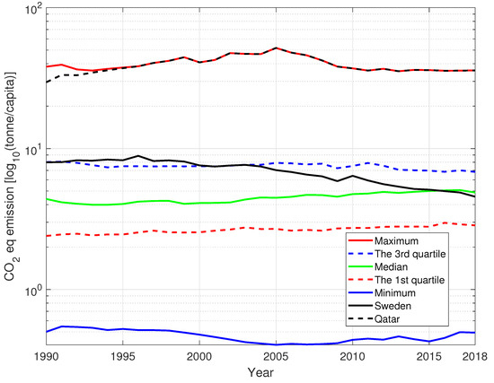
Figure 4.
Percentile plot of total GHG emission per countries. Based on country emissions data, percentile values can be calculated each year to obtain the maximum, the third quartile, median, first quartile, and minimum functions. The figure can be used to determine the role of a country in damaging the environment. In this example, Qatar has the highest damaging potential during the past few years. However, Sweden has reduced the GHG emission significantly from the third quartile to the median.
Although the global average annual growth slowly started to dampen, the growth is still remarkable. The countries that contributed the most to the global GHG emissions increase are China (420 (+3.1%)), followed by Indonesia (50 (+5.5%)). In contrast, countries and regions that decreased the most are the European Union (−3.0%), the United States (−1.7%), Japan and South Korea. However, the per capita emissions enable the comparison between countries considering the size of countries’ activities [37]. According to Olhoff and Christensen [52], in order to meet the target 1.5 °C-consistent pathway, the global average per capita consumption emission should reach 2.1 per capita in 2030.
Figure 5 represents the total emission per capita in the world. From 2003 to 2011, the average annual growth in emission was 3.2%; however, the great recession in 2008 had a significant effect on global GHG emission. Since 2012, the global annual growth started to slow down, and the total per capita decreased until 2016. Since then, global GHG emissions have started to increase. This rebound is considered mainly due to a new increase in global coal consumption of 0.4% in 2017 and 1.7% in 2018 after three years of decreases (−0.1%, −2.5% and −1.5%). The decrease in coal consumption is partly based on the shift of the United States and the European Union from power plants to natural gas and renewable power generation [37]. In the following years, due to the COVID-19 crisis, a short-term decrease in GHG emission is expected (2–4 ), after which emissions are assumed to follow pre-2020 growth trends [52]. The global GHG emissions are dominated by fossil share, which steadily increased since 1990. From 2000 to 2009, the global annual GHG emissions increased 2.4% per year; then, it decreased to by half: 1.4% annual growth since 2010. The increase slowed down to 0.3% in 2015 and 2016, which was followed by 1.3% and 3.0% in 2017 and 2018. However, the global emission growth is slowing, and country dynamics significantly differ. Organisation of Economic Co-operation and Development (OECD) economies indicate declining emission trends, while non-OECD economies’ emission is increasing [58]. The largest share of GHG emissions in 2018 was the Energy sector (37.22 ), followed by Agriculture (5.82 ), Industrial Processes (2.90 ), Waste (1.61 ) and Bunker Fuels (1.31 ). Each sector faces challenges to reduce environmental impact and mitigate climate change.
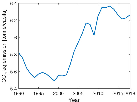
Figure 5.
The total equivalent emission per capita in the world. The great recession in 2008 can be well recognized.
Figure 6 indicates the sectoral distribution of greenhouse gas emission per country. Five major sectors are considered, namely: Agriculture, Bunker Fuel, Energy, Industrial Processes and Waste. Within the Energy sector, six subsectors are defined: Building, Electricity/Heat, Fugitive Emissions, Manufacturing/Construction, Other Fuel Combustion and Transportation. This sectoral breakdown enables us to identify the driving sectors of climate change that need to be addressed. Furthermore, this percentile-based representation enables us to easily identify where the majority of countries are located regarding their emission rates. Targeted analysis can also be made for each country, as their performance in each sector can be analyzed.
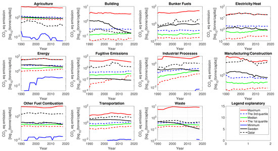
Figure 6.
Percentile plot of total GHG emission per countries. Based on country emissions data, percentile values can be calculated each year to obtain the maximum, the third quartile, median, first quartile, and minimum functions. The figure can be used to determine the role of a country in damaging the environment. In this example, Qatar has the highest damaging potential during the past years. However, Sweden has reduced the GHG emission significantly from the third quartile to the median.
The Agriculture, Bunker Fuel, Energy, Industrial Processes and Waste Sectors are profoundly interconnected and cover the aspects of energy supply, energy demand, non-energy related process emissions, and land-based emissions and removals, which is also reflected in the global, regional, country-wise and sectoral greenhouse gas emissions [59]. The highest absolute increase in GHG emission between 2010 and 2018 was in Eastern Asia (2.6 ), which is followed by Southern Asia (1.1 ). In the case of developed regions—North America, Latin America and developed countries in the Asia Pacific—the greenhouse gas emission growth is slowly dampening (+0.1%/yr. +0.1%/yr, +0.4%/yr). The only region where the total GHG emission declined during this period is Europe (−0.3 , −0.8%/yr). “A combination of stable demand, energy efficiency improvements, fuel switching and a scale-up of renewables has led to an absolute decline in emissions” [59]. In these developed counties, the highest emission rate came from energy systems, industry and transportation. However, a respective decline has been observed in the Energy sector in Europe and North America since 2010 (−1.8%/yr and −1.5%/yr). For developing regions, such as Africa, Latin America and Southeast Asia, the highest emission rate is originated from agriculture and land-use changes (deforestation) [59]. Still, recently, there has been an increase in shares of transportation, energy systems and industry sectors. Eastern and Southern Asia are also associated with these sectors, and their rates exceed 4%/yr. It is unclear when the global peak in GHG emissions will be reached.
The Energy sector is the most pollutant sector in the majority of countries. Regarding the Energy sector, 25% of countries emitted at least 1.598 per capita in 2018, which is higher than in other sectors. Between 1990 and 2018, 25% of the countries emitted 1.84% more concerning the Energy sector, while the third quartile (75% of the countries) had an approximate 0.22 decrease. Within the Energy sector, the Electricity/Heat subsector has the highest share, which is followed by Transportation and Manufacturing/Construction. Countries’ energy consumption and connected emissions are dependent on their geographic features and general energy transition strategies [60]. Sweden was slightly under the third quartile in 2018 with 3.497 per capita, which is half of its emission in 1990. On the contrary, Qatar has the highest emission regarding the Energy sector with 34.288 per capita. Transition strategies and energy planning policies and methods require multilevel governance to support the synergies between different sectors and develop sustainable energy systems based on renewables, energy-efficient applications and the decentralization of energy generation [61]. “There are three possible pathways for decarbonisation of heating, decarbonisation of gas, replacing gas by decarbonised district heating and replacing gas by decarbonised electricity but the choice is dependent on general energy transition” [60]. The electrification of transportation is a challenging and promising solution to achieve sustainable energy development in cities [62]. In order to accomplish 100% renewable energy systems, different sectors must be integrated flexibly along with capture and utilization technologies [63].
The percentile plot of the Agriculture sector shows a steady slow decrease in GHG emissions per capita. In 2018, between 25% and 75% of the countries emitted within the range of 0.553–0.879 per capita. Sweden’s emissions approximate the median with 0.7115 per capita (2018), while Qatar belongs to the 25% of countries with the lowest emission originate from the Agriculture sector. Agriculture is considered the second most contributing sector to climate change, while it suffers from significant impacts of climate change. The past 50 years resulted in doubled freshwater withdrawal and halved agricultural land per capita (from 1. 4 to 0.7 ha) by agriculture intensification [64]. In order to meet the Paris Agreement and keep the global temperature increase below 1.5–2.0 °C, there is a need for “decarbonisation [to] include enhancing carbon sequestration, increasing bioenergy production, reducing emission intensity of agriculture and shifting diets” [65].
The Industrial Processes sector shows a slight increase concerning most of the countries’ (75%) GHG emission per capita; however, the maximum value in 2018 (4.372 per capita) doubled compared to the base year 1990 (2.375 per capita). In 2018, Sweden approximated the median with 0.243 per capita, while Qatar is within the 25% of countries with the highest emission per capita (1.071 ) concerning the Industrial Processes sector. Industry-related emission sources are based on the production of metals, chemicals, cement and other basic materials [59]. These production processes are often inefficient and not sustainable and required to reduce emissions from an industrial operation, while the industry should be compatible to supply transformational technologies and infrastructure [66]. These transformations will likely be deployed in waves, for which previous investments in research and development, pilot projects and infrastructure are needed [67].
The emission of the Waste sector has remained steady since 1990, and there is no significant change in the values of the quartiles. Sweden performed a significant reduction of its emission concerning the Waste sector. In 2018, Sweden emitted 0.102 per capita, which is 76% lower compared to 1990 (0.4311 per capita, which was higher than 75% of countries’ emission in that year). According to a study [68], there is a relationship between the amount of generated waste and the level of income (wealth); however, this relationship can be non-linear. Recycling, composting, and incinerating processes may replace standard landfills as the income grows. “A de-linking relationship among wealth and waste may emerge, with major positive effects on the environmental quality” [68]. Waste policy efforts should focus on changing behaviors and firms’ decisions concerning waste production. Otherwise, the gap between policy objectives to slow down climate change and the implementation will emerge [68].
Concerning the Bunker Fuels sector, the quartile values seem to remain steady. Bunker fuels are used in the maritime industry to power ship engines. The International Maritime Organization (IMO) Initial GHG Strategy in 2018 assigned a goal to reduce GHG emissions from ships by at least 50% in absolute terms by 2050 compared to 2008 [69]. In order to reach this target, energy transition is required to shift from fossil bunker fuels to alternative bunker fuels with low, ultimately zero GHG emissions. Potential zero-carbon fuels options can include synthetic diesel, novel biofuels, and fuels that involve hydrogen. Its production from natural gas is in conjunction with 100% carbon capture and storage and its production from 100% non-biogenic renewable electricity [70]. Bunker Fuel is the only sector where Sweden increased its GHG emissions between 1990 and 2018 (by 225%). Qatar increased its emission 4.5 times regarding the Bunker Fuel sector (from 0.734 to 3.278 per capita). Both Sweden and Qatar belong to the top 25% of countries that emit the most concerning the Bunker Fuel sector.
Based on the sectoral contributions in Figure 6, the analysis of the time series of the countries allows the shift of energy as one of the leading sectors in the energy transition of the countries, which requires the active governmental support of the increase of the spread of renewable energy sources. The transition trajectories are both technologically driven and provide social context [71]. In the case of electricity/heat, as also an outstanding sectoral contribution, emphasis should be placed on energy-saving measures in buildings, the data recording, and processing tasks; artificial intelligence techniques for a scalable energy transition will be important in the future [72].
3.2. Evaluation of the Consistency of the Sector-Wise Transitions
The consistency of the transitions was evaluated based on the statistical properties of the time series tested by the Leybourne–McCabe and Runs tests. As Table 1 shows, we calculated the number of countries where the time series of the GHG emission of a given sector is random and stationer. As can be seen, the randomness and the stationary-related properties are well correlated, as both criteria measure how systematic the changes are. The results highlight that the Waste sector shows the most predictable trends, while the Fugitive emissions and Bunker Fuels sectors show the less systematic changes.

Table 1.
The number of countries where the GHG emission-related time series of a given sector show random or stationary behavior.
Table 1 shows that most of the time-series data are not random, but the picture is much more divided in terms of stationarity. In the case of industrial sectors, countries must identify potential development areas, or more precisely, focus on the progress made in the real engine rooms of the technological revolution [73]. Decision makers should focus on financial sustainability issues within the agricultural industry [74]. In addition, it is necessary to accurately determine the load of agricultural farms, grid demands and the nexus of electricity markets [75]. Technological systems of agriculture, as manure management, nitrogen efficiency, precision agriculture and decentralized supply carry high transitional potential [76]. In the building sector, only a comprehensive set of sufficient, efficient and renewable energy sources makes it possible to achieve the global climate goals [77]. The energy conservation [78] standard for buildings, the comprehensive assessment system of the environmental efficiency of buildings [79], helps the planning of mitigation solutions for this sector. Bunker fuels with zero-carbon emissions, such as biofuels, hydrogen and ammonia, as well as synthetic carbon-based fuels, contribute to the modernization of the domestic energy and industrial infrastructure [70]. Solutions such as carbon prices applied to bunker fuel in the range of USD 10–50/tonne of carbon dioxide can increase the cost of sea transportation by 0.4–16% [80]. Residential rooftop photovoltaic (PV) systems can solve the problem of increasing electricity demand for sustainable energy systems [81]. Switching to renewable energy sources can reduce GHG emissions, water consumption and electricity system costs [82]. Nevertheless, we must be aware of the environmental impacts of renewable power plants [83], which must be planned already during GHG mitigation. The modernization of industrial processes, energy efficiency, regulation of the burning of agricultural waste and fuel conversion are important aspects in the reduction of pollutants that cause industrial air pollution [84]. Achievements in industrial transformation and non-fossil fuel development have defined China’s leading provinces in reducing carbon emissions [85]. In the case of transport, it is possible to reduce motorized passenger activity, speed up the development of public transport and electrification, and decarbonize the energy production system. In this sector, a single mitigation technology or delivery method alone is not sufficient; a mixture of solutions is needed [86].
The highlight that a mixture of solutions is needed can be extended to the design of global GHG mitigation strategies, as countries need to identify potential development areas and systematic changes (shown in Figure 7) in the energy transition through the time series of sectoral contributions.
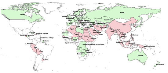
Figure 7.
The world map of countries that have changed their emission systematically. The red color stands for systematic emission increase, the green color denotes systematic emission decrease, and the white color means no systematic changes.
Based on the number of sectors that show systematically an increase or decrease, the countries were also classified into three categories that are presented in Figure 7. The resulted map shows clear clusters of countries that follow similar development strategies.
An interesting future research direction is to forecast countries’ GDP and GHG emissions relations, identifying their future location on their individual Kuznets curve. However, this is a complex task, since countries’ economic regressions, such as the Great Recession in 2008 and COVID-19 from 2019, and ever-changing legal and social expectations significantly impact both GDP and GHG emissions.
3.3. Country-Wise Comparison Based on the Trends on the Improvement-Related Variables
The performance of countries is compared based on the defined improvement-related variables and presented in the context of recent studies. Figure 8 and Figure 9 indicate how much countries changed their emissions production per capita between 1990 and 2018. The major drivers of GHG/capita are energy intensity, economic growth and carbon factor; however, energy intensity also serves as one of the major drivers of the decrease in GHG/capita [87].
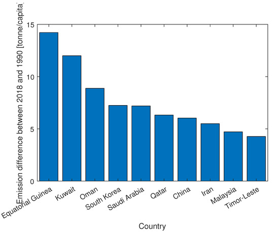
Figure 8.
The difference between the GHG emissions measured in 2018 and 1990. The top ten most increased countries. The absolute scale can focus on the global contribution of countries to GHG emission.
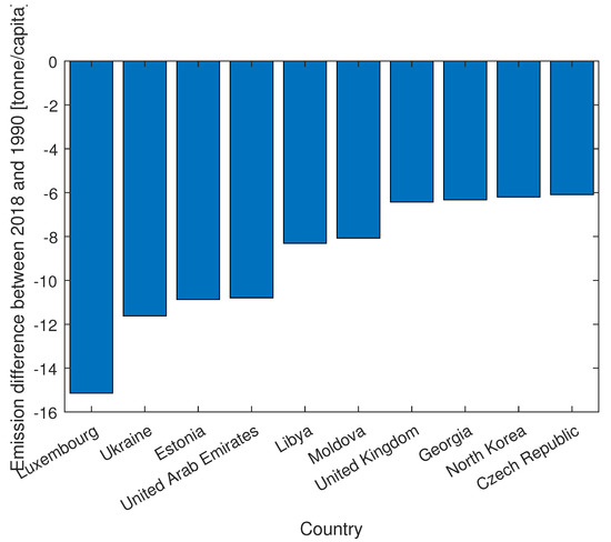
Figure 9.
The difference between the GHG emissions measured in 2018 and 1990. The top ten countries that have decreased their GHG emissions the most. The absolute scale can focus on the global contribution of countries to GHG emission.
In Figure 8, the top ten most emitting countries are listed. Equatorial Guinea increased its GHG emission per capita by 14.22 between 1990 and 2018, which is followed by Kuwait (12), Oman (8.88) and South Korea (7.24). China is in 6th place based on its overall increase in GHG emission per capita. The top ten countries regarding the most significant decrease in GHG emissions produced between 1990 and 2018 are shown in Figure 9. Luxembourg decreased its emission level by 15.14 per capita, which is followed by Ukraine (11.62), Estonia (10.87) and the United Arab Emirates (10.79).
Figure 10 represents the countries ranking order based on their GHG reduction percentage in 2018 compared to 1990. The dots represent the countries, which are grouped and color-coded according to their reduction percentage. The dashed red baseline GHG emission represents the emission level of 1990, while the green line indicates the target level based on the Green Deal to reach at least 55% GHG reduction compared to 1990 levels. Countries’ ISO codes from right to left and top to bottom are in order with the countries’ location in each group. Although the European Green Deal was specially designed for European Union member states, the Green Deal-based utility function can be extended globally to examine countries’ reduction performances over the years and provide a comparative overview. Furthermore, predictions can be made for countries to see whether they will reach the target for 2030 or not, based on the trend of change in GHG emissions. Countries under the target level are the following: Gabon, Georgia, Zambia, Kyrgyzstan, Moldova, Ukraine, Gambia, and North Korea. The low emission rate of these countries is caused by weak economic development. From 1990 until around 2000, there was a massive drop in the country’s GDP and GHG emission levels. Since then, the increase in their GDP has stagnated.
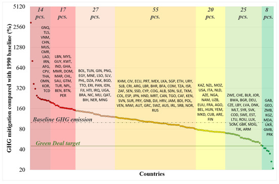
Figure 10.
The actual GHG reduction percent in 2018 compared with 1990. The European Green Deal targets for 2030 to at least a 55% GHG reduction compared with 1990 levels. Country groups are color-coded based on their reduction percent. The ISO codes from right to left and top to bottom are in order with the countries’ location in each group.
The origin of the low emission countries’ performance is an interesting question. Does it originate from economic stability and investments in environmental protection, renewable energy-based energy systems and technologies, or is it caused by an economic recession that significantly reduced GHG emissions (such as in 2008)? In the latter case, the future performance of those countries will depend on their development strategies. There are two possible pathways: one is that due to economic development, they invest in sustainable pathways to keep their emission low, or otherwise, their emission level will rebound to the previous level. To accurately analyze the reason of the decrease or increase, an in-depth country-specific analysis is needed.
A recent study assessed the level of the sustainable energy and climate development of the EU countries over a 10-year period based on 14 indicators describing the energy, environment, economy, and society dimensions and considered the priority areas of the European Green Deal and goals 7 and 13 of the 2030 Agenda for Sustainable Development [88]. The countries have been classified based on their sustainable energy and climate development factor. As a result, the greatest sustainable energy and climate development is associated with Sweden, Denmark, France and Austria, while there are low levels of sustainable development in, e.g., Bulgaria, Poland and Cyprus [88]. According to a study forecasting GHG emissions for the Baltic States, the current national climate policies are insufficient to achieve the 2030 Green Deal emission reduction targets [16]. Furthermore, for more effective long-term energy and climate policies, specific targets for transport, industry, services, agriculture and household sectors are needed [16].
Figure 11 indicates countries’ GHG emission changes between 1990 and 2018 as well as their 2018 emission level. This visualization enables us to analyze the performance more accurately. If countries are located close to 0 on both the y and x-axes, their performance stagnates. Countries in the left bottom corner decreased their emission level significantly and kept their emission levels low, such as in Ukraine, Monaco, etc. Although countries located closer to the left upper corner (Luxembourg, United Arab Emirates, etc.) decreased their emissions, their emission level in 2018 was still high. In contrast, countries that approximate the right upper corner are increasing their initially high GHG emission level (Qatar, Bahrain, Kuwait etc.). Although emission reductions can be observed in several countries, they are inconsistent, and more emphasis needs to be placed on reducing emissions from transport [89].
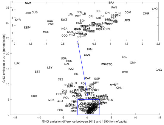
Figure 11.
This figure shows the GHG emission change between 2018 and 1990 of each country. Moreover, the actual level in 2018 can also be considered. Luxembourg reduced significantly in the studied period, but the country still produces a high level of GHG emissions. However, Ukraine also significantly reduced the GHG emissions, and the country produced a low level of GHG emissions in 2018. Meanwhile, Qatar increased the GHG emission very significantly and produced a high level of GHG emission in 2018. More countries are concentrated around zero on the positive side, which means that many countries have increased their emission slightly. However, this can be increased significantly in the future.
Based on the most effective examples of specific emissions presented in Figure 9 and quantifying the distance from the 1990 base year (Figure 10), we recommend that countries set realistic targets for both specific emissions and aggregate emissions to enhance their improvement in the efficiency transition.
3.4. Kuznets Analysis
Figure 12 shows the Kuznets curves of countries by assuming a relationship between economic development (GDP) and greenhouse gas emissions per capita. “Economic growth has a strong positive effect on carbon dioxide, sulfur dioxide, and industrial greenhouse gas (GHG) emissions, but weaker effects on non-industrial GHG emissions and concentrations of particulates” [90]; as well as inadequate funding and financial instruments, lack of advanced technologies are affecting the environment and industry-related GDP [91]. According to the environmental Kuznets curve theory, during the early stages of development, higher economic growth results in environmental degradation, but beyond a certain point, higher economic growth may lead to environmental improvements, which results in an inverted U shape [42]. Three stages of development in an economy are defined concerning the Kuznets curve, namely, pre-industrial economy, industrial economy and post-industrial economy. “GDP is clearly a significant factor underpinning changes in GHG emissions” [92]. However, GDP per capita has a heterogeneous effect on GHG emissions, which indicates that general economic development alone cannot reduce GHG emissions; it is necessary but not a sufficient condition. The environmental and energy policies, strategies and measures are essential factors in reducing GHG emissions; however, its effectiveness and efficiency vary across GHG distribution [33]. In order to achieve greater reductions in greenhouse gas emissions, pro-environmental and country-specific national policies are required [33], and the adaptation of energy efficiency measures in all sectors of the economy have to be accelerated [16].
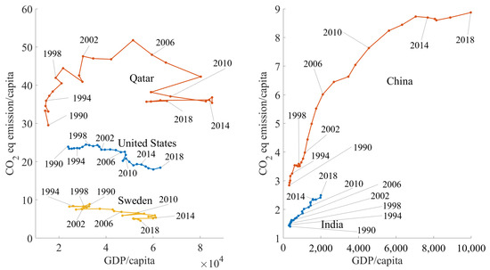
Figure 12.
The Kuznets curves of GHG emission changes. By comparing the practical and theoretical Kuznets curves, the level of development of a given country can be assumed. Developing countries are before the turning point, such as China or India. However, Qatar appears to be already after the turning point, and GHG emissions are on a decreasing trend.
Figure 12 provides a clear representation of countries’ transition trajectories based on their individual Kuznets curves. Developing countries, such as China and India, have not reached the turning point yet, while the United States, Sweden and Qatar appear to be in the third stage with decreasing environmental degradation impact. Notably, the economic regressions, such as the great recession between 2008 and 2009, significantly appears. Developing countries as China and India have a comparative advantage in carbon-intensive production and goods, which increase the aggregate economic growth [91]. “Developing countries using their comparative advantage in exchange for modernised technological transfer, innovations, and partnership on clean energy technologies would reduce stress on natural resource and improve environmental sustainability, thus, reducing environmental pollution” [93]. The emissions rate within China is dependent on the income levels as urban residents tend to pay for a cleaner environment, while in the countryside, residents with low income have a higher environmental deteriorating impact [94]. In The U.S.-China Joint Announcement on Climate Change in November 2014, China pledged to peak its GHG emissions around 2030 and increase the share of non-fossil fuels in primary energy consumption to around 20% by 2030. This agreement is reinforced in The Paris Agreement in December 2015. According to the study of Song et al., potential pathways toward a fossil energy-related GHG emission peak for China have been identified based on an integrated input–output simulation model, which estimated no peak timing before 2030 only in one scenario where industrial restructuring and intensified energy consumption and GHG emission reduction policies are involved [95]
On the contrary, the high-income economy tends to invest more in research and development and promote the implementation of renewable energy sources to replace fossil energy sources [96]. Nordic countries, including Sweden, are leaders in low-carbon energy transition, which is nicely represented by the fact that Sweden’s emissions are lower than those in 1960 [97]. It is underlined by the study of Dolge et al., which identifies Sweden as a benchmark for achieving the highest impact on GHG emissions reductions [16]. In the USA, a paradigm shift can be observed from high-energy intensive and carbon-intensive industries toward information and service-intensive industries with advanced technologies, which promote environmental awareness and regulations and policies [94]. Qatar’s high emission rate originates from the oil, gas, electricity and desalination production [98]. Although Qatar’s economy has been heavily dependent on natural gas and oil revenues, it is worrying that these fossil fuel resources will be depleted in the near future [99]. Qatar is rich in renewable resources such as wind and solar; however, in 2020, its total renewable energy consumption was lower than 0.005 exajoules compared to the total energy consumption of 1.71 [2]. The transition from natural gas to solar input is expected to significantly impact Qatar’s GHG emission and environment [99]. One of the central pillars of the Qatar National Vision 2030 is the environmental protection and harmony between economic growth and social development [100]. Despite significant increases in GDP and population growth, the reduction of carbon intensity and energy intensity have to be equally considered to create positive synergies and achieve higher cumulative GHG emission reductions [16].
Furthermore, the Kuznets curve of the world is also identified, as shown in Figure 13. Due to the aggregation of countries’ performances, shifts and inequalities can be due to very well or very poorly performing countries. Based on the visual interpretation, the great economic crises are well identifiable. Significant impacts on both the GDP and environmental pollution are observable, and after the crises, when economies started to strengthen, environmental degradation had an increasing effect on the planet. Even though more and more economies are preparing strategies to reach carbon neutrality, being aware of environmental risks and investing in environmentally friendly technologies and solutions, the world does not seem to have reached the tipping point yet.
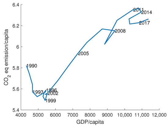
Figure 13.
Kuznets function of the world.
4. Conclusions
This paper presented novel techniques for exploring countries’ GHG emissions. The analysis was executed based on the CAIT dataset included on the Climate Watch website from 1990 to 2018 about per capita emissions of countries. The time series were analyzed with a percentile-based method to highlight the position of the countries in the global contribution of GHG emissions. Moreover, the sectoral breakdown of GHG emissions was also considered, and improvement-related variables were generated to compare countries quantitatively and underpin the identification of realistic targets for the energy transition. The background and the results of the analyses were presented relative to current research, which enrich the context of the study. The analyses underlined the importance of sectoral targets, policy making and social factors to achieve more sufficient transition.
The case study presented mainly two counties, Sweden and Qatar. Qatar has peaked at the maximum GHG value in the examined time, while Sweden could significantly decrease their GHG emission. The sectoral breakdown of the data has shown that the primary sector that contributed to the most GHG emission was the energy in Qatar. Sweden could decrease in many sectors, but the mostly noteworthy is in Waste and Building.
The environmental Kuznets curve reflected that Sweden has a post-industrial economy, where GHG emission reduction is expected. Qatar went through the whole economic phase over the past year, implying that GHG emission reduction is expected.
The time-series analysis of most countries shows the application of systematic reduction policy.
A future research direction is to develop an algorithm that can continuously monitor how far the achievement of GHG emission goals could be based on the actual trends. Another aim could be to investigate how the environmental Kuznets curve is influenced by various explanatory variables: for example, climate change mitigation actions, population, etc. Based on the analyzes, the need for the improved use of renewable energies and the development of energy efficiency in buildings, as well as the identification and integration of external variables (sustainability (SDG) efforts, new international laws and regulations, carbon capture solutions, carbon offsets, and carbon credits) into databases are of paramount importance for GHG reduction.
Author Contributions
Conceptualization, J.A and V.S.; methodology, R.C. and T.C.; software, R.C.; validation, V.S.; formal analysis, R.C. and J.A.; investigation, T.C.; writing—original draft preparation, T.C. and R.C.; writing—review and editing, J.A and V.S.; visualization, R.C.; supervision, V.S. and J.A.; project administration, J.A.; funding acquisition, J.A. All authors have read and agreed to the published version of the manuscript.
Funding
This work was supported by the National Multidisciplinary Laboratory for Climate Change (RRF-2.3.1-21-2022-00014) and by the TKP2021-NVA-10 project with the support provided by the Ministry for Innovation and Technology of Hungary from the National Research, Development and Innovation Fund, financed under the 2021 Thematic Excellence Programme funding scheme.
Institutional Review Board Statement
Not applicable.
Informed Consent Statement
Not applicable.
Data Availability Statement
The time-series data of greenhouse gas emissions is based on the CAIT dataset included in the Climate Watch website at https://www.climatewatchdata.org/data-explorer/historical-emissions?historical-emissions-data-sources=cait&historical-emissions-gases=&historical-emissions-regions=&historical-emissions-sectors=&page=1, accessed on 9 August 2021. The emissions production (referred to as emissions) per capita values are calculated based on the population data taken from the World Bank Database, from where the GDP data were also downloaded https://www.kaggle.com/ibrahimmukherjee/gdp-world-bank-data, accessed on 13 July 2021.
Conflicts of Interest
The authors declare no conflict of interest.
References
- Stocker, T. Climate Change 2013: The Physical Science Basis: Working Group I Contribution to the Fifth Assessment Report of the Intergovernmental Panel on Climate Change; Cambridge University Press: Cambridge, UK, 2014. [Google Scholar]
- Dale, S. BP Statistical Review of World Energy 2021; BP Plc: London, UK, 2021. [Google Scholar]
- Desa, U. Transforming Our World: The 2030 Agenda for Sustainable Development; United Nations: New York, NY, USA, 2016.
- Rogelj, J.; Den Elzen, M.; Höhne, N.; Fransen, T.; Fekete, H.; Winkler, H.; Schaeffer, R.; Sha, F.; Riahi, K.; Meinshausen, M. Paris Agreement climate proposals need a boost to keep warming well below 2 C. Nature 2016, 534, 631–639. [Google Scholar] [CrossRef] [PubMed]
- Tian, J.; Yu, L.; Xue, R.; Zhuang, S.; Shan, Y. Global low-carbon energy transition in the post-COVID-19 era. Appl. Energy 2022, 307, 118205. [Google Scholar] [CrossRef] [PubMed]
- Bogdanov, D.; Ram, M.; Aghahosseini, A.; Gulagi, A.; Oyewo, A.S.; Child, M.; Caldera, U.; Sadovskaia, K.; Farfan, J.; Barbosa, L.D.S.N.S.; et al. Low-cost renewable electricity as the key driver of the global energy transition towards sustainability. Energy 2021, 227, 120467. [Google Scholar] [CrossRef]
- Foley, A.; Smyth, B.M.; Pukšec, T.; Markovska, N.; Duić, N. A review of developments in technologies and research that have had a direct measurable impact on sustainability considering the Paris agreement on climate change. Renew. Sustain. Energy Rev. 2017, 68, 835–839. [Google Scholar] [CrossRef]
- Santika, W.G.; Anisuzzaman, M.; Bahri, P.A.; Shafiullah, G.; Rupf, G.V.; Urmee, T. From goals to joules: A quantitative approach of interlinkages between energy and the Sustainable Development Goals. Energy Res. Soc. Sci. 2019, 50, 201–214. [Google Scholar] [CrossRef]
- Grubler, A.; Wilson, C.; Bento, N.; Boza-Kiss, B.; Krey, V.; McCollum, D.L.; Rao, N.D.; Riahi, K.; Rogelj, J.; De Stercke, S.; et al. A low energy demand scenario for meeting the 1.5 C target and sustainable development goals without negative emission technologies. Nat. Energy 2018, 3, 515–527. [Google Scholar] [CrossRef]
- Sikora, A. European Green Deal–legal and financial challenges of the climate change. In Proceedings of the Era Forum; Springer: Berlin/Heidelberg, Germany, 2021; Volume 21, pp. 681–697. [Google Scholar]
- Tao, R.; Umar, M.; Naseer, A.; Razi, U. The dynamic effect of eco-innovation and environmental taxes on carbon neutrality target in emerging seven (E7) economies. J. Environ. Manag. 2021, 299, 113525. [Google Scholar] [CrossRef]
- Lovell, H.; Liverman, D. Understanding carbon offset technologies. New Political Econ. 2010, 15, 255–273. [Google Scholar] [CrossRef]
- Wilberforce, T.; Olabi, A.; Sayed, E.T.; Elsaid, K.; Abdelkareem, M.A. Progress in carbon capture technologies. Sci. Total Environ. 2021, 761, 143203. [Google Scholar] [CrossRef]
- Ashley, M.J.; Johnson, M.S. Establishing a secure, transparent, and autonomous blockchain of custody for renewable energy credits and carbon credits. IEEE Eng. Manag. Rev. 2018, 46, 100–102. [Google Scholar] [CrossRef]
- Chang, M.; Thellufsen, J.Z.; Zakeri, B.; Pickering, B.; Pfenninger, S.; Lund, H.; Østergaard, P.A. Trends in tools and approaches for modelling the energy transition. Appl. Energy 2021, 290, 116731. [Google Scholar] [CrossRef]
- Dolge, K.; Blumberga, D. Economic growth in contrast to GHG emission reduction measures in Green Deal context. Ecol. Indic. 2021, 130, 108153. [Google Scholar] [CrossRef]
- Hainsch, K.; Löffler, K.; Burandt, T.; Auer, H.; del Granado, P.C.; Pisciella, P.; Zwickl-Bernhard, S. Energy transition scenarios: What policies, societal attitudes, and technology developments will realize the EU Green Deal? Energy 2022, 239, 122067. [Google Scholar] [CrossRef]
- Chen, X.; Yang, F.; Zhang, S.; Zakeri, B.; Chen, X.; Liu, C.; Hou, F. Regional emission pathways, energy transition paths and cost analysis under various effort-sharing approaches for meeting Paris Agreement goals. Energy 2021, 232, 121024. [Google Scholar] [CrossRef]
- Hojnik, J.; Ruzzier, M. What drives eco-innovation? A review of an emerging literature. Environ. Innov. Soc. Transitions 2016, 19, 31–41. [Google Scholar] [CrossRef]
- Althor, G.; Watson, J.E.; Fuller, R.A. Global mismatch between greenhouse gas emissions and the burden of climate change. Sci. Rep. 2016, 6, 20281. [Google Scholar] [CrossRef]
- Squalli, J. Disentangling the relationship between immigration and environmental emissions. Popul. Environ. 2021, 43, 1–21. [Google Scholar] [CrossRef]
- Gillenwater, M. Forgotten carbon: Indirect CO2 in greenhouse gas emission inventories. Environ. Sci. Policy 2008, 11, 195–203. [Google Scholar] [CrossRef]
- Kumar, A.; Singh, P.; Raizada, P.; Hussain, C.M. Impact of COVID-19 on greenhouse gases emissions: A critical review. Sci. Total Environ. 2022, 806, 150349. [Google Scholar] [CrossRef]
- Twine, R. Emissions from Animal Agriculture—16.5% Is the New Minimum Figure. Sustainability 2021, 13, 6276. [Google Scholar] [CrossRef]
- Baloch, M.A.; Danish; Qiu, Y. Does energy innovation play a role in achieving sustainable development goals in BRICS countries? Environ. Technol. 2021, 43, 2290–2299. [Google Scholar] [CrossRef] [PubMed]
- Hamid, I.; Alam, M.S.; Kanwal, A.; Jena, P.K.; Murshed, M.; Alam, R. Decarbonization pathways: The roles of foreign direct investments, governance, democracy, economic growth, and renewable energy transition. Environ. Sci. Pollut. Res. 2022, 29, 49816–49831. [Google Scholar] [CrossRef] [PubMed]
- Ćetković, J.; Lakić, S.; Živković, A.; Žarković, M.; Vujadinović, R. Economic analysis of measures for GHG emission reduction. Sustainability 2021, 13, 1712. [Google Scholar] [CrossRef]
- Gençer, E.; Torkamani, S.; Miller, I.; Wu, T.W.; O’Sullivan, F. Sustainable energy system analysis modeling environment: Analyzing life cycle emissions of the energy transition. Appl. Energy 2020, 277, 115550. [Google Scholar] [CrossRef]
- Wardekker, A.; Lorenz, S. The visual framing of climate change impacts and adaptation in the IPCC assessment reports. Clim. Chang. 2019, 156, 273–292. [Google Scholar] [CrossRef]
- Mukhopadhyay, U.; Pani, R. Emission and sectoral energy intensity: A variance decomposition analysis. Manag. Environ. Qual. Int. J. 2022, 33, 955–974. [Google Scholar] [CrossRef]
- Climate Watch, GHG Emissions Excluding Land-Use Change and Forestry, CAIT Data. Available online: https://www.climatewatchdata.org/data-explorer/historical-emissions?historical-emissions-data-sources=cait&historical-emissions-gases=&historical-emissions-regions=&historical-emissions-sectors=&page=1 (accessed on 9 August 2021).
- Phiri, A. Economic growth, Environmental degradation and business cycles in Eswatini. Bus. Econ. Horizons 2019, 15, 490–498. [Google Scholar]
- Borozan, D. Revealing the complexity in the environmental Kuznets curve set in a European multivariate framework. Environ. Dev. Sustain. 2021, 24, 9165–9184. [Google Scholar] [CrossRef]
- Grossman, G.M.; Krueger, A.B. Economic growth and the environment. Q. J. Econ. 1995, 110, 353–377. [Google Scholar] [CrossRef]
- Agency, E.P. Inventory of U.S. Greenhouse Gas Emissions and Sinks: 1990–2019; Technical Report; United States Environmental Protection Agency: Washington, DC, USA, 2021.
- GDP World Bank Data. Available online: https://www.kaggle.com/ibrahimmukherjee/\gdp-world-bank-data (accessed on 13 July 2021).
- Olivier, J.; Peters, J. Trends in Global CO2 and Total Greenhouse Gas Emissions; PBL Netherlands Environmental Assessment Agency: Hague, The Nethwelands, 2020. [Google Scholar]
- Kleinbaum, D.G.; Klein, M. Survival Analysis; Springer: New York, NY, USA, 2010; Volume 3. [Google Scholar]
- Gibbons, J.D.; Chakraborti, S. Nonparametric Statistical Inference; CRC Press: Boca Raton, FL, USA, 2014. [Google Scholar]
- Chen, Z. A note on the runs test. Model Assist. Stat. Appl. 2010, 5, 73–77. [Google Scholar] [CrossRef]
- Leybourne, S.J.; HcCabe, B. Modified stationarity tests with data-dependent model-selection rules. J. Bus. Econ. Stat. 1999, 17, 264–270. [Google Scholar]
- Stern, D.I. The environmental Kuznets curve. In Oxford Research Encyclopedia of Environmental Science; Oxford University Press: Oxford, UK, 2017. [Google Scholar]
- Shahbaz, M.; Sinha, A. Environmental Kuznets curve for CO2 emissions: A literature survey. J. Econ. Stud. 2019, 46, 106–168. [Google Scholar] [CrossRef]
- Destek, M.A.; Ulucak, R.; Dogan, E. Analyzing the environmental Kuznets curve for the EU countries: The role of ecological footprint. Environ. Sci. Pollut. Res. 2018, 25, 29387–29396. [Google Scholar] [CrossRef]
- Wang, Q.; Wang, X.; Li, R. Does urbanization redefine the environmental Kuznets curve? An empirical analysis of 134 Countries. Sustain. Cities Soc. 2022, 76, 103382. [Google Scholar] [CrossRef]
- Katsoulakos, N.; Misthos, L.M.; Doulos, I.G.; Kotsios, V. Environment and Development. In Environment and Development; Elsevier: Amsterdam, The Netherlands, 2016; pp. 499–569. [Google Scholar]
- Sarkodie, S.A.; Ozturk, I. Investigating the environmental Kuznets curve hypothesis in Kenya: A multivariate analysis. Renew. Sustain. Energy Rev. 2020, 117, 109481. [Google Scholar] [CrossRef]
- Kaika, D.; Zervas, E. The Environmental Kuznets Curve (EKC) theory—Part A: Concept, causes and the CO2 emissions case. Energy Policy 2013, 62, 1392–1402. [Google Scholar] [CrossRef]
- Churchill, S.A.; Inekwe, J.; Ivanovski, K.; Smyth, R. The environmental Kuznets curve in the OECD: 1870–2014. Energy Econ. 2018, 75, 389–399. [Google Scholar] [CrossRef]
- Boubellouta, B.; Kusch-Brandt, S. Testing the environmental Kuznets Curve hypothesis for E-waste in the EU28+ 2 countries. J. Clean. Prod. 2020, 277, 123371. [Google Scholar] [CrossRef]
- Yao, S.; Zhang, S.; Zhang, X. Renewable energy, carbon emission and economic growth: A revised environmental Kuznets Curve perspective. J. Clean. Prod. 2019, 235, 1338–1352. [Google Scholar] [CrossRef]
- Olhoff, A.; Christensen, J.M. Emissions Gap Report 2020; UNEP DTU Partnership; 2020; Available online: https://www.unep.org/emissions-gap-report-2020 (accessed on 24 July 2022).
- Di Giulio, A.; Fuchs, D. Sustainable consumption corridors: Concept, objections, and responses. GAIA-Ecol. Perspect. Sci. Soc. 2014, 23, 184–192. [Google Scholar] [CrossRef]
- Saujot, M.; Le Gallic, T.; Waisman, H. Lifestyle changes in mitigation pathways: Policy and scientific insights. Environ. Res. Lett. 2020, 16, 015005. [Google Scholar] [CrossRef]
- Fanning, A.L.; O’Neill, D.W.; Büchs, M. Provisioning systems for a good life within planetary boundaries. Glob. Environ. Chang. 2020, 64, 102135. [Google Scholar] [CrossRef]
- Qatar, G. Qatar national vision 2030. In Doha, General Secretariat for Development; 2008. Available online: https://www.psa.gov.qa/en/qnv1/pages/default.aspx (accessed on 24 July 2022).
- Government Offices of Sweden. Sweden’s Long-Term Strategy for Reducing Greenhouse Gas Emissions; 2020. Available online: https://unfccc.int/documents/267243 (accessed on 24 July 2022).
- Le Quéré, C.; Korsbakken, J.I.; Wilson, C.; Tosun, J.; Andrew, R.; Andres, R.J.; Canadell, J.G.; Jordan, A.; Peters, G.P.; van Vuuren, D.P. Drivers of declining CO2 emissions in 18 developed economies. Nat. Clim. Chang. 2019, 9, 213–217. [Google Scholar] [CrossRef]
- Lamb, W.F.; Wiedmann, T.; Pongratz, J.; Andrew, R.; Crippa, M.; Olivier, J.G.; Wiedenhofer, D.; Mattioli, G.; Al Khourdajie, A.; House, J.; et al. A review of trends and drivers of greenhouse gas emissions by sector from 1990 to 2018. Environ. Res. Lett. 2021, 16, 073005. [Google Scholar] [CrossRef]
- Duić, N.; Krajačić, G. Decarbonisation of Heating—Towards 2050. In Solar Energy Conversion in Communities; Springer: Cham, Germany, 2020; pp. 177–178. [Google Scholar]
- Dobravec, V.; Matak, N.; Sakulin, C.; Krajačić, G. Multilevel governance energy planning and policy: A view on local energy initiatives. Energy, Sustain. Soc. 2021, 11, 2. [Google Scholar] [CrossRef]
- Yuan, M.; Thellufsen, J.Z.; Lund, H.; Liang, Y. The electrification of transportation in energy transition. Energy 2021, 236, 121564. [Google Scholar] [CrossRef]
- Mikulčić, H.; Skov, I.R.; Dominković, D.F.; Alwi, S.R.W.; Manan, Z.A.; Tan, R.; Duić, N.; Mohamad, S.N.H.; Wang, X. Flexible Carbon Capture and Utilization technologies in future energy systems and the utilization pathways of captured CO2. Renew. Sustain. Energy Rev. 2019, 114, 109338. [Google Scholar] [CrossRef]
- Bombelli, A.; Di Paola, A.; Chiriacò, M.V.; Perugini, L.; Castaldi, S.; Valentini, R. Climate change, sustainable agriculture and food systems: The world after the Paris agreement. In Achieving the Sustainable Development Goals Through Sustainable Food Systems; Springer: Cham, Germany, 2019; pp. 25–34. [Google Scholar]
- Svensson, J.; Waisman, H.; Vogt-Schilb, A.; Bataille, C.; Aubert, P.M.; Jaramilo-Gil, M.; Angulo-Paniagua, J.; Arguello, R.; Bravo, G.; Buira, D.; et al. A low GHG development pathway design framework for agriculture, forestry and land use. Energy Strategy Rev. 2021, 37, 100683. [Google Scholar] [CrossRef]
- Davis, S.J.; Lewis, N.S.; Shaner, M.; Aggarwal, S.; Arent, D.; Azevedo, I.L.; Benson, S.M.; Bradley, T.; Brouwer, J.; Chiang, Y.M.; et al. Net-zero emissions energy systems. Science 2018, 360, eaas9793. [Google Scholar] [CrossRef]
- Rissman, J.; Bataille, C.; Masanet, E.; Aden, N.; Morrow III, W.R.; Zhou, N.; Elliott, N.; Dell, R.; Heeren, N.; Huckestein, B.; et al. Technologies and policies to decarbonize global industry: Review and assessment of mitigation drivers through 2070. Appl. Energy 2020, 266, 114848. [Google Scholar] [CrossRef]
- Magazzino, C.; Mele, M.; Schneider, N.; Sarkodie, S.A. Waste generation, wealth and GHG emissions from the waste sector: Is Denmark on the path towards circular economy? Sci. Total Environ. 2021, 755, 142510. [Google Scholar] [CrossRef] [PubMed]
- Joung, T.H.; Kang, S.G.; Lee, J.K.; Ahn, J. The IMO initial strategy for reducing Greenhouse Gas (GHG) emissions, and its follow-up actions towards 2050. J. Int. Marit. Safety, Environ. Aff. Shipp. 2020, 4, 1–7. [Google Scholar] [CrossRef]
- Englert, D.; Losos, A.; Raucci, C.; Smith, T. The Potential of Zero-Carbon Bunker Fuels in Developing Countries; International Bank for Reconstruction and Development/The World Bank: Washington, DC, USA, 2021. [Google Scholar]
- Defeuilley, C. Energy transition and the future(s) of the electricity sector. Util. Policy 2019, 57, 97–105. [Google Scholar] [CrossRef]
- Sayed-Mouchaweh, M. Artificial Intelligence Techniques for a Scalable Energy Transition: Advanced Methods, Digital Technologies, Decision Support Tools, and Applications; Springer: Cham, Switherlands, 2020. [Google Scholar]
- Hanna, R.; Victor, D.G. Marking the decarbonization revolutions. Nat. Energy 2021, 6, 568–571. [Google Scholar] [CrossRef]
- Sroufe, R.; Watts, A. Pathways to Agricultural Decarbonization: Climate Change Obstacles and Opportunities in the US. Resour. Conserv. Recycl. 2022, 182, 106276. [Google Scholar] [CrossRef]
- Aghajanzadeh, A.; Therkelsen, P. Agricultural demand response for decarbonizing the electricity grid. J. Clean. Prod. 2019, 220, 827–835. [Google Scholar] [CrossRef]
- Sovacool, B.K.; Bazilian, M.; Griffiths, S.; Kim, J.; Foley, A.; Rooney, D. Decarbonizing the food and beverages industry: A critical and systematic review of developments, sociotechnical systems and policy options. Renew. Sustain. Energy Rev. 2021, 143, 110856. [Google Scholar] [CrossRef]
- Camarasa, C.; Mata, É.; Navarro, J.P.J.; Reyna, J.; Bezerra, P.; Angelkorte, G.B.; Feng, W.; Filippidou, F.; Forthuber, S.; Harris, C.; et al. A global comparison of building decarbonization scenarios by 2050 towards 1.5–2 °C targets. Nat. Commun. 2022, 13, 3077. [Google Scholar] [CrossRef]
- Ma, M.; Ma, X.; Cai, W.; Cai, W. Carbon-dioxide mitigation in the residential building sector: A household scale-based assessment. Energy Convers. Manag. 2019, 198, 111915. [Google Scholar] [CrossRef]
- Murakami, S.; Levine, M.D.; Yoshino, H.; Inoue, T.; Ikaga, T.; Shimoda, Y.; Miura, S.; Sera, T.; Nishio, M.; Sakamoto, Y.; et al. Overview of energy consumption and GHG mitigation technologies in the building sector of Japan. Energy Effic. 2009, 2, 179–194. [Google Scholar] [CrossRef]
- Halim, R.A.; Smith, T.; Englert, D.P. Understanding the Economic Impacts of Greenhouse Gas Mitigation Policies on Shipping: What Is the State of the Art of Current Modeling Approaches? In World Bank Policy Research Working Paper; World Bank Group: Washington, DC, USA, 2019. [Google Scholar]
- Monna, S.; Abdallah, R.; Juaidi, A.; Albatayneh, A.; Zapata-Sierra, A.J.; Manzano-Agugliaro, F. Potential Electricity Production by Installing Photovoltaic Systems on the Rooftops of Residential Buildings in Jordan: An Approach to Climate Change Mitigation. Energies 2022, 15, 496. [Google Scholar] [CrossRef]
- Gupta, A.; Davis, M.; Kumar, A. An integrated assessment framework for the decarbonization of the electricity generation sector. Appl. Energy 2021, 288, 116634. [Google Scholar] [CrossRef]
- Sebestyén, V. Renewable and Sustainable Energy Reviews: Environmental impact networks of renewable energy power plants. Renew. Sustain. Energy Rev. 2021, 151, 111626. [Google Scholar] [CrossRef]
- Munsif, R.; Zubair, M.; Aziz, A.; Zafar, M.N. Industrial air emission pollution: Potential sources and sustainable mitigation. In Environmental Emissions; IntechOpen: London, UK, 2021. [Google Scholar]
- Mi, Z.; Sun, X. Provinces with transitions in industrial structure and energy mix performed best in climate change mitigation in China. Commun. Earth Environ. 2021, 2, 182. [Google Scholar] [CrossRef]
- Milovanoff, A.; Minet, L.; Cheah, L.; Posen, I.D.; MacLean, H.L.; Balasubramanian, R. Greenhouse gas emission mitigation pathways for urban passenger land transport under ambitious climate targets. Environ. Sci. Technol. 2021, 55, 8236–8246. [Google Scholar] [CrossRef]
- Zheng, X.; Streimikiene, D.; Balezentis, T.; Mardani, A.; Cavallaro, F.; Liao, H. A review of greenhouse gas emission profiles, dynamics, and climate change mitigation efforts across the key climate change players. J. Clean. Prod. 2019, 234, 1113–1133. [Google Scholar] [CrossRef]
- Tutak, M.; Brodny, J.; Bindzár, P. Assessing the Level of Energy and Climate Sustainability in the European Union Countries in the Context of the European Green Deal Strategy and Agenda 2030. Energies 2021, 14, 1767. [Google Scholar] [CrossRef]
- Lamb, W.F.; Grubb, M.; Diluiso, F.; Minx, J.C. Countries with sustained greenhouse gas emissions reductions: An analysis of trends and progress by sector. Clim. Policy 2022, 22, 1–17. [Google Scholar] [CrossRef]
- Stern, D.I. The environmental Kuznets curve after 25 years. J. Bioecon. 2017, 19, 7–28. [Google Scholar] [CrossRef]
- Sarkodie, S.A.; Strezov, V. A review on environmental Kuznets curve hypothesis using bibliometric and meta-analysis. Sci. Total Environ. 2019, 649, 128–145. [Google Scholar] [CrossRef]
- Agency, E.E. Why Did Greenhouse Gas Emissions Decrease in the EU between 1990 and 2012? European Environment Agency: Copenhagen, Denmark, 2014.
- Sarkodie, S.A.; Strezov, V. Effect of foreign direct investments, economic development and energy consumption on greenhouse gas emissions in developing countries. Sci. Total Environ. 2019, 646, 862–871. [Google Scholar] [CrossRef] [PubMed]
- Sarkodie, S.A.; Strezov, V. Empirical study of the environmental Kuznets curve and environmental sustainability curve hypothesis for Australia, China, Ghana and USA. J. Clean. Prod. 2018, 201, 98–110. [Google Scholar] [CrossRef]
- Song, J.; Yang, W.; Wang, S.; Higano, Y.; Fang, K. Exploring potential pathways towards fossil energy-related GHG emission peak prior to 2030 for China: An integrated input-output simulation model. J. Clean. Prod. 2018, 178, 688–702. [Google Scholar] [CrossRef]
- Bulut, U. Testing environmental Kuznets curve for the USA under a regime shift: The role of renewable energy. Environ. Sci. Pollut. Res. 2019, 26, 14562–14569. [Google Scholar] [CrossRef]
- Urban, F.; Nordensvärd, J. Low carbon energy transitions in the Nordic countries: Evidence from the environmental Kuznets curve. Energies 2018, 11, 2209. [Google Scholar] [CrossRef]
- Qatar—International Energy Data and Analysis; U.S. Energy Information Administration: Washington, DC, USA, 2015.
- Salahuddin, M.; Gow, J. Effects of energy consumption and economic growth on environmental quality: Evidence from Qatar. Environ. Sci. Pollut. Res. 2019, 26, 18124–18142. [Google Scholar] [CrossRef]
- Tan, T.; Al-Khalaqi, A.; Al-Khulaifi, N. Qatar national vision 2030. Sustain. Dev. Apprais. Gulf Reg. 2014, 19, 65. [Google Scholar]


Publisher’s Note: MDPI stays neutral with regard to jurisdictional claims in published maps and institutional affiliations. |
© 2022 by the authors. Licensee MDPI, Basel, Switzerland. This article is an open access article distributed under the terms and conditions of the Creative Commons Attribution (CC BY) license (https://creativecommons.org/licenses/by/4.0/).