Abstract
Motivation: This paper presents the high contact resistance (HCR) and rotor bar faults by an extraction method for an induction motor using Discrete Wavelet Transform (DWT) and Artificial Neural Network (ANN). The root mean square (RMS) and mean features are obtained using DWT, and ANN is used for classification using activation functions. Activation provides output by assigning the specific input with respect to the transfer function according to the nature and type of the activation function. Method: The faulty conditions are induced using MATLAB by adopting the motor current signature analysis (MCSA) method to achieve current signature signals of the healthy and faulty motors. Results: The DWT technique has been applied to obtain fault-specific features of the average continuously varying signal (RMS) and an average of the data points (mean) at levels 5, 7, 8, and 9, followed by ANN to classify the faults for condition monitoring. Utility: The utility of the results is to reduce unscheduled downtime in the industry, thus saving revenue and reducing production losses. This work will help provide support to ensure early indication of faults in induction motors under operating conditions, enabling in-service engineers to take timely preventive measures as part of the availability of resources in IoT-enabled systems. Application: Resource availability and cybersecurity are becoming vital in an environment that supports the Internet of Things (IoT) as the essential components of Industry 4.0 scenarios. The novelty of this research lies in the implementation of high contact resistance and rotor bar faults using DWT and ANN with different activation functions to achieve accuracy up to 98%.
1. Introduction
Background: Availability in a secure IoT-enabled environment refers to the ease with which an organization’s critical data, applications, and resources can be accessed by authorized users. Industry motors bear the features of being simple in design, robust in construction, reliable in operation, low in cost, and easy to maintain, and accordingly, are widely used in industry. However, induction motors are also prone to various faults [1,2,3], leading to their failure, which put the availability of resources at risk. If not detected in time, these faults will lead to irremediable mechanical failures. The objective of this research is, therefore, to develop a technique for detecting faults that appear on operational motors. The main faults detected and analyzed during induction-motor processing are related to stator faults, broken rotor bars, and air-gap eccentricity-related faults that have been investigated and reported extensively in the literature [4,5,6,7]. The motivation of this paper is derived from Internet resources and articles exploring faults using none-ANN techniques.
Motivation: Operational motors, as resources, generate data, and it is important that induction motors as data resources are easily accessible to authorized users bearing IoT-enabled features. In particular, high contact resistance (HCR) and rotor bar faults have been considered in this study in order to investigate their availability as data resources. Because of these potential faults, it is crucial to monitor motor health and maintenance issues. Thus, the presentation as a platform for safe operation from the IoT-enabled scenario perfective is important, and refers to the ease with which organizations’ critical data, applications, and resources can be accessed by their respective users [8].
State-of-art works: Multiple machine condition-monitoring strategies have already been investigated in the literature [9,10], including partial discharge, vibration analysis, current signature investigation, magnetic flux, and acoustic noise monitoring. However, the Motor Current Signature Analysis (MCSA) is considered to be the most commonly reported technique applied to fault analysis [11,12]. The phase current signal contains current motor operation-dependent components, which are the by-product of unique rotating flux components. In the supply current, the occurrence of faults brings about changes that have specific harmonic contents which are specific to the faults that occur. The MCSA technique works on stator current measurements to detect the harmonics generated under faulty conditions, which, although unwanted, are used for fault analysis. Furthermore, the MCSA provides current spectra that possess potential information for the detection of electrical and mechanical faults. In this investigation, motor parameters, mainly current, have been acquired for the three phases of a motor in operation.
Novelty and contribution: The novelty of this work is the current spectrum that has been analyzed over a wide range of distinct current patterns that could serve as signature values for fault detection. The two faults under investigation in this work are: (1) the high resistance connection fault (21%), and (2) the broken rotor bar fault (7%), both categories are caused by manufacturing defects [13,14]. The fault analysis of the induction motor is done through high resolution spectral analysis of the low frequency signals associated with various fault categories [15]. Statistical features extraction followed by a mix of classification algorithms are used in [16]. Induction motors make up between 40 to 60% of any industrial site’s electrical loads employed. The online sensor-based detection of induction motors faults through the sensing of stray flux components containing information of relevance for the diagnosis of faults in induction motors is shown in [17]. The unbalanced supply voltage and inter-turns short circuits are studied in [18] through thermal behavior of the motors. The analysis of supply current signals under faulty condition of specific number of rotor bars as time–frequency features is commonly used in recent work [19].
The remainder of the paper is organized as follows. Section 2 consists of the work related to the two faults. Section 3 describes induction motors. Discrete Wavelet Transform (DWT) for fault detection is explained Section 4. Section 5 explains the ANN Classifier. Results are given in Section 6. The paper’s conclusions are presented in Section 7.
2. Related Work
From a review of the literature, it was concluded that many different techniques have been used to diagnose machine faults in industry, and various classification methods have been implemented to obtain satisfactory results. Table 1 has been adopted from the state-of-the-art paper, tabulated in [20], and presents the results obtained through artificial neural network (ANN) classification. A maximum of 95% accuracy was previously achieved, but details of the hidden layers and activation function were not mentioned. Conversely, in the present study, more than 96% accuracy has been attained at different Debauches levels, with detailed information reported on the hidden layers and activation functions. Moreover, stator winding faults, bearing faults, broken rotor bar faults, and eccentricity are the primary research interests in previous studies [21], whereas in this current research, HCR and broken rotor bar faults are discussed.

Table 1.
Accuracy tabulated from the literature review versus a classification approach.
2.1. High Connection-Resistance (HCR) Fault
As the name implies, an HCR fault relates to poor and loose contacts with localized heat due to unbalance, and failures are associated with this fault, resulting in reduced efficiency and reliability. This fault can be located in circuit breakers, motor starter terminals, or other similar points in the power circuit where contacts and connections are involved. As the above-mentioned faults increase, the motor temperature also rises, and is associated with onset of insulation damage. According to standard electrical testing, an effective method of measuring HCR is to measure phase-to-phase resistance between the three phases.
In this research, a HCR fault has been designed in MATLAB software by connecting a 1 kΩ, 10 W resistor in series in one phase of the induction motor model, as shown in Figure 1. It may be noted that HCR faults can be modelled by resistance in the kΩ to MΩ range.
2.2. Rotor Bar Fault
When a rotor bar fault occurs in the motor and the current flowing through the broken bars stops, the broken bars stop sharing torque. This results in a burden on the healthy bars. In cases where there are many broken rods, the motor will not start. Broken rotor bar (BRB) fault occurs due to magnetic stresses, thermal stresses, contamination, or abrasion and wearing away of the rotor due to a lack of maintenance. Cracks from high temperatures are also a possible consequence. To investigate the rotor bar fault induced in this study, the MATLAB Simulink environment was designed, as shown in Figure 2.
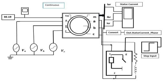
Figure 2.
Rotor bar fault in MATLAB Simulink Environment A–C stator phases and a–c rotor phases.

Figure 1.
High contact resistance (HCR) fault in a MATLAB Simulink environment. A–C shows stator phases.
Figure 1.
High contact resistance (HCR) fault in a MATLAB Simulink environment. A–C shows stator phases.

Artificial intelligence (AI) procedures may be developed to diagnose faults in their early stages. The ANN model was preferred in this study, and discrete wavelet transform (DWT) was used to obtain features at different levels, for which the ANN classifier was trained accordingly. Finally, the test data were fed into the ANN classifier, which, along with the algorithmic details and steps, are illustrated in Figure 3.
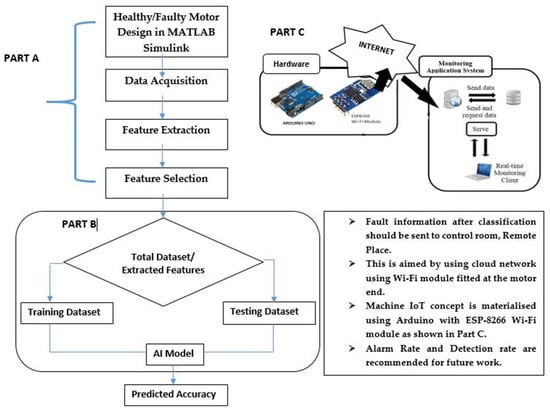
Figure 3.
Proposed Algorithm Flowchart (Quality Improved also enlarged-300 dpi).
Figure 3 represents the proposed steps that were followed in this research. Part A represents the steps of signal analysis for feature extraction and selection. The features are acquired using wavelet db-4 transform technique, as shown in Figure 3. Part B shows how to extract relevant features to train the ANN model to predict the results, while Part C shows the feature of enabling IoT with a Wi-Fi module with the motor by adapting the technology [24] with less interference [25] and also with fast computational performance [26].
In an IoT-enabled environment, communication between the induction motors (resources) and central monitoring station is facilitated by two-way communication via a radio communication system that operates in the cloud, as shown in Figure 3. The features signifying faults become recognizable as indicators of the availability of inductors for use in industry. Alternatively, this makes it possible for employees with expert knowledge to gain easy access to motors in order to assess their availability as resources.
3. Induction Motor Modelling
Induction motor modelling MATLAB software was used to design the motor model in this research. The 5.4 HP (4 kW), 400 V, 50 Hz, 1430 RPM induction motor was designed in a MATLAB Simulink environment, as shown in Figure 4. HCR and rotor bar faults are illustrated in Figure 1 and Figure 2, respectively. From the simulated motor design, the data were acquired from a healthy motor and a fault-induced motor.
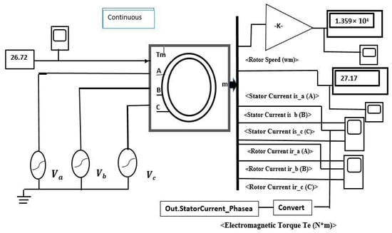
Figure 4.
Healthy Motor SIMULINK model with A–C stator phases.
4. Discrete Wavelet Transform (DWT)
This paper focuses on extracting features of the mean and RMS for fault diagnosis using DWT. These features were used as input into the ANN model [27,28]. They were investigated in this study, as shown in Figure 5, then analyzed to obtain the most relevant information from the signals for further processing. The main contributions of this study are that we propose a method to convert time-series data, such as current signals, into grayscale images, using the EWT transformation coupled with the deep CNN model for fault diagnosis [29]. The use of ML algorithms and the DL to machine failure diagnosis is reported in [22]. Discrete wavelet transform is mostly used where analysis of the time–frequency domain signal is required. It is the most efficient tool for extracting transient-based nature signals. Discrete wave transform computes the series of wavelet coefficients, approximation for low frequency feature points, and detail coefficients for high frequency feature points [30]. In a very closely related report, an ensemble machine learning-based fault classification scheme using DWT to compare both raw and filtered separately through wavelet decomposition was reported [31]. In practical terms, DWT can be implemented by using a pair of low-pass and high-pass filters. Wavelet transform is formed from a wavelet of a prototype signal—called a ‘mother’ or ‘single modeling’ wavelet y (t)—through shifting operation and dilation. This relationship is shown in the following equation. For the case of Discrete Wavelet Transform, the mother wavelet is shifted and scaled by the powers of two, where j and k are scale and shift parameters, both representing integer values. Here, the mother wavelet is shifted and scaled by a power of two.
where j is scaling parameter, k represents shifting parameter, t is time and ψ (t) represents the function of mother wavelet. Mathematically, DWT can be computed by convolving the signal with the dilated, reflected, and normalized version of the mother-wavelet . The Equation (3) is result of convolution of the samples with the mother-wavelet.
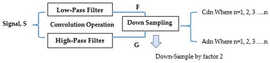
Figure 5.
Decomposition procedure for the DWT: representation of the low-pass and high-pass filters, convolving with signal ‘S’. (Figure Reduced in size-300 dpi).
Recalling the wavelet coefficient γ of a signal is a projection of onto a wavelet, and let be a signal of length , in the case of child wavelet in the discrete family above.
By fixing j at a scale, so that is a function of k only, by the Equation (2), can be viewed as a convolution of with reflected, dilated and normalized version of mother-wavelet, , sampled at the points 1, ,. But this is precisely what the detail coefficients give at different levels of j for DWT as shown in the Figure 6, Figure 7 and Figure 8. Therefore an appropriate choice for the signals, g[n] and h[n], the detail coefficients of the filter bank correspond exactly to a wavelet coefficient of discrete set of child wavelet for a given mother wavelet .
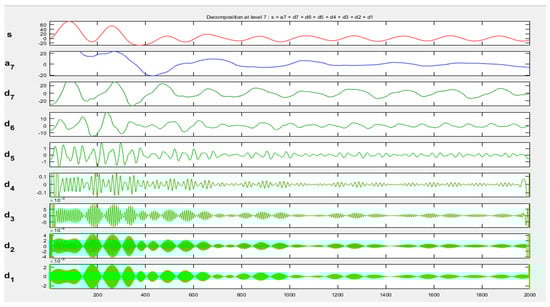
Figure 6.
Representation of DWT Approximation Coefficients and Detail Coefficients of Healthy Phase-A Currents with 2000 samples.
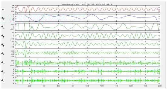
Figure 7.
Representation of DWT approximation coefficients and detail coefficients of HCR fault in Phase-A currents with 2000 samples.
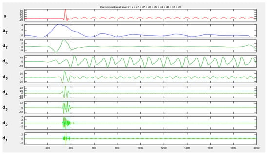
Figure 8.
Representation of DWT approximation coefficients and detail coefficients of a faulty signal rotor bar fault in Phase-A currents with 2000 samples.
Filters decompose the signals into approximation and detail coefficients, and their computation is given as [17]
The above equations can be more precisley described by the given convolution approach (6), (7).
The DWT decomposition process of 2-level DWT is illustrated in Figure 5, Equation (2), presented above, helps compute DWT, and Equations (4) and (5) represent the low- and high-pass filters, respectively, showing the high-frequency and low-frequency components. The outputs give the detail coefficients (from the high-pass filter) and approximation coefficients (from the low-pass filter).
Designation of Frequency Band
Each Debauches wavelet db-4 contains multiple levels. As a 10 kHz frequency was used to sample the current signals in this research, a single sample of 10 kHz was distributed across 9 db-4 wavelet levels. The distribution of frequency band is tabulated in Table 1. All wavelet levels except for 7, 8 and 9 were discarded, because these levels possessed no valuable information. Moreover, the signals with line noise at 50 Hz were also discarded, as noise reduction clarified the target signals more effectively. Table 2 shows distribution frequency bands.
Table 2.
Distribution of frequency bands.
In this research, DWT 1-dimension analysis was used for the healthy and faulty motor signals, and the following graphs were derived from the 2000 data samples gathered. Figure 6 represents the DWT approximation levels (a7 only, using level-7 alone) and detail coefficient levels (d1–d7) of a current healthy conditions signal in Phase A, using just seven levels of decomposition. It may be concluded that on starting, the induction motor current showed greater amplitude, due to higher torque, which gradually settled down into a steady state from 800 samples onward. Signals were decomposed into seven levels to obtain high- and low-frequency information about the current signal. The authors in [31] report successful implementation of the DWT technique, with accuracy more than 99%. In comparison, this research work also achieves more than 98% accuracy, possibly because of the dataset used. The authors in [23] also present successful fault diagnosis using DWT and achieve claimable accuracy. The authors in Refs. [32,33] show techniques other than the DWT, such as data augmentation-based, feature learning-based and classifier designing-based, using different datasets, calling them intelligent diagnosis models with deep networks to conclude how to reduce the consumption of computing time. However, these strategies are complex and need improvement for data generation ability and data dimensionality issues based on the different dataset conditions. Finally, the authors in [34] report on the identification of faults using coupled neuron-based approach, mainly focusing on enhancing the weak useful signature, and not applying a classifier-based approach to find accuracy using a relatively complex approach compared to the proposed approach, where the condition of fault is the main interest.
Figure 7 displays the DWT coefficient levels (a7 only) and detail coefficient levels (d1–d7) for the HCR fault in the Phase-A current. The fault was analyzed and the detail coefficients, d1, d2, d3, and d4, were found to contain less information and fewer features, as most of the noise was contained by d1, d2, d3, and d4. All detail coefficients, representing most of the high-frequency content and the approximate coefficients containing low-frequency information about the current signals, were obtained at level 7, with a clearly visible difference between the healthy and damaged motor signals.
Figure 8 displays the DWT coefficients of Phase-A currents with rotor bar fault, wherefrom, it may be concluded that initially, the motor was running normally. A rotor bar fault was subsequently introduced at 350 samples, due to which, the motor displayed the fault with spikes at corresponding coefficients. This indicated that the fault had been detected, and the DWT coefficients had received frequency information about the currents. The signal contamination was due to the rotor bar fault. Moreover, feature points were extracted using DWT. The signal and approximation coefficients at level 1 are very identical. However, they become gradually different at higher and higher levels. A similar tendency can be visibly noted in the case of the bearing fault using DWT and ensemble machine learning algorithms [31].
Figure 9 represents the feature points for a healthy motor in Phase-A at level 9, and similar features were extracted for the remaining faults at different levels, using DWT. In this research, the mean and RMS features were investigated. In addition, Figure 6 and Figure 8 show the detail and approximation coefficients for healthy motor and rotor bar fault signals, containing both low-frequency and high-frequency content information about the approximation and detail coefficients, respectively.
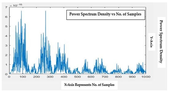
Figure 9.
Healthy motor phase: a feature point representation with 1000 samples. (Figures Titled-300 dpi).
Figure 10 and Figure 11 display the features obtained using DWT at level 9. These features are the composite form of different detail levels, as represented in Figure 6.
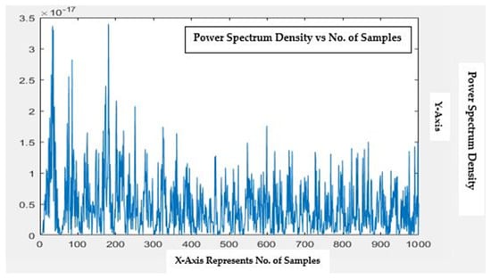
Figure 10.
High contact resistance fault in Phase-A: Representation of feature points with 1000 samples. (Figures Titled-300 dpi).
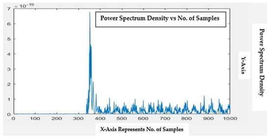
Figure 11.
Rotor bar fault in Phase-A: Representation of feature points with 1000 samples (Figures Titled-300 dpi).
5. ANN Classifier
The concept of ANN is to classify deniable features that characterize target parameters in real-world applications. Artificial neural networks are brain-inspired neural network (NN) systems. The Neural Network (NN) works similar to neurons in our nervous system, and is capable of learning from past data; the ANN is able to learn from data and provide responses in the form of classifications. It is the most widely used form of AI [27], mostly preferred for fault detection and diagnosis. An ANN can be trained by causing the interconnected nodes (called neurons) to learn in a way that resembles that of the human brain by recognizing speech patterns and tendencies in images. The behavior is defined by the weights assigned to these interconnections, ensuring that the desired task is performed correctly. Artificial neurons networks are excellent tools for identifying complex problems. The multi-layer feed-forward NN with a back-propagation training algorithm is the classic NN proposed in this study. Neural Networks have already been successfully applied and proven suitable for fault detection [22,28,29,30,31], and pseudocode has been provide in Appendix A.
In this research, supervised learning was applied to train both healthy and faulty motors [22,27,28,29,30,31]. There are three main components of an ANN: the input layer, hidden layers, and output layers, as shown in Figure 12. In an ANN, layers possess nodes, and these nodes relate to the nodes in the next layer. Moreover, each connection has proportionated weights, considered as the effect of the nodes on the layers. The hidden layers contain information that is transformed onto higher order node layers. Each node is associated with a predefined activation function, which will determine whether the node will be activated on a node in a higher layer. The way in which it is activated will depend on the summarized values obtained by multiplying the values of the nodes with their associated weights. The neuron in an ANN is the computational unit that takes x1, x2, and x3 as inputs, as well as an intercept term. The output ‘y’ is obtained by
where the activation function is represented by ‘f’, and often chosen to be the sigmoid function (as in this research), different activation functions are investigated by taking 21 hidden layers and 11 epochs. ‘W’ is the ANN model weight, while ‘b’ is the scalar value, known as the bias. Here, Equation (8) was used to compute output ‘y’ of the ANN. Performance indicator parameters for NN model are shown in Figure 13, below, where it can be seen that the overall cross entropy error of the trained NN is 0.59872 at epoch 10. The model was trained for an HCR fault at level 9, with RMS features. During the analysis of results for different activation functions and size of layers, it was observed that the designing of Neural Network could be accomplished with a lesser number of hidden layers without affecting the accuracy. In this work, at 21 hidden layers, good accuracies are obtained for all transfer functions while the rest of the parameters are kept the same.
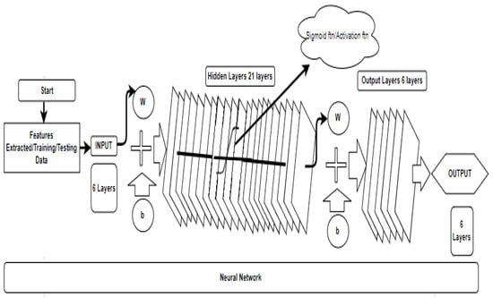
Figure 12.
Neural network (NN) model.
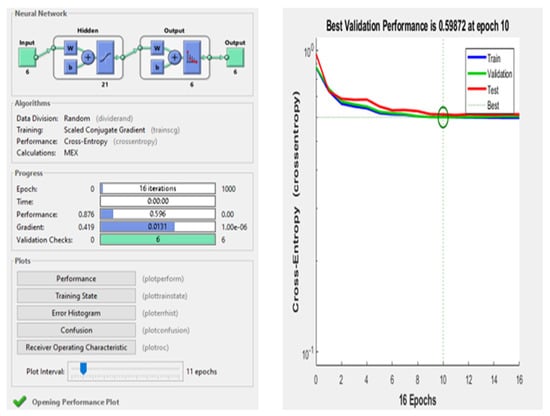
Figure 13.
Neural network model performance parameters and cross-entropy error.
Figure 13 shows that validation and training have similar characteristic curves with efficient testing. As in NNs, the hyper-parameters were tuned to provide a high quality solution for the ANN model and the number of epochs consisted of numerical figures—indicating the number of times that the entire dataset was propagated forward and backward through an NN. The epochs were chosen to control the number of complete passes through the training dataset. These epochs were divided into batches for processing.
It may be pointed out that all the ROC’s figures (Train, Test, and Validation, etc.) if accommodated in a few plots, will result in the cramping of many of our interests, considering we do not have any ZOOMING option in the tool used.
From the above figure, it is concluded that all faults are classified with 76% accuracy, All ROC curves point out that the grey diagonal line of ROC means that the samples lying on this line show that the proportion of correctly classified samples is the same as the proportion of incorrectly classified samples.
- Class-1 (Healthy Phase A)
- Class-2 (Healthy Phase-B)
- Class-3 (Healthy Phase-C)
- Class-4 (Faulty Phase-A) Rotor Bar/High-Contact Resistance
- Class-5 (Faulty Phase-B) Rotor Bar/High-Contact Resistance
- Class-6 (Faulty Phase-C) Rotor Bar High-Contact Resistance
In the ROC-training section, the six different classes have been classified. During the validation process, each class has transmit data according to its specific feature type. Different colours represent the different phases and types of classes. The third section describes the testing of ROC using a different scheme of classes, and the classification was categorized according to features. The tangent/diagonal line was received in ALL-ROC sections, which shows that if the line of different Phases exists above the ROC diagonal grey coloured line, it means the samples are correctly and properly classified with a true positive rate, else, if the lines of Phases exist below the diagonal lines, it means the samples are classified incorrectly, and do not belong to the same Phases. From Figure 14, it can be concluded that some of the samples of the Phases (features) are correctly classified and some samples are incorrectly classified, therefore, the accuracy obtained is 76.0%, as shown in the Confusion Matrix.
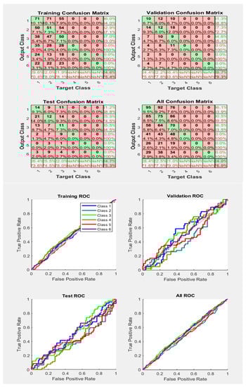
Figure 14.
Neural Network Model ROC (Receiver Operating Characteristics) and Confusion Matrix for OSS Train Fcn/Activation Function at level 9 (RMS) Features for High Contact Resistance Fault with 76.0% Accuracy. Grey line shows diagonal of the ROC for indicating Class 1–6 lines are lying above or below or on it.
From Figure 15, it is clear that with an accuracy of 82.6%, compared to Figure 14, with 76.0%, we have obtained a more appropriate classification of the different faults and Phases with the same number of samples and activation function. Almost all Phases lines drawn are received above the grey diagonal line, and this line is supposed to represent the threshold line for the ROC Curves.
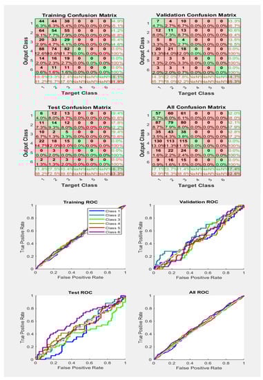
Figure 15.
Neural Network Model ROC (Receiver Operating Characteristics) and Confusion Matrix for OSS TrainFcn/Activation Function at level 9 (RMS) Features for High Contact Resistance Fault with 82.6% Accuracy. Grey line shows diagonal of the ROC for indicating Class 1–6 lines are lying above or below or on it.
Figure 16 makes the things more clear by showing the grey diagonal line and almost all Phase lines with their samples very appropriately classified with a good True Positive rate by obtaining an accuracy level of about 92.2%, which, as compared to the results obtained in Figure 14 and Figure 15, are better. Moreover, a single Phase line is below that diagonal line, meaning that only the Phase samples are incorrectly classified.
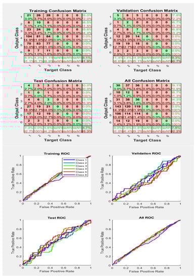
Figure 16.
Neural Network Model ROC (Receiver Operating Characteristics) and Confusion Matrix for OSS TrainFcn/Activation Function at level 9 (RMS) Features for High Contact Resistance Fault with 92.2% Accuracy. Grey line shows diagonal of the ROC for indicating Class 1–6 lines are lying above or below or on it.
Similarly, Figure 17 represents less accurate accuracy results compared to Figure 16, and the ROC curves also represent that some Phases are classified appropriately, while others have incorrect classification. However, this time, the training/activation function is ‘lm’.
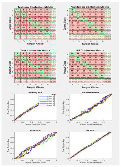
Figure 17.
Neural Network Model ROC (Receiver Operating Characteristics) and Confusion Matrix for LM TrainFcn/Activation Function at level 9 (RMS) Features for High Contact Resistance Fault with 74.8% Accuracy. Grey line shows diagonal of the ROC for indicating Class 1–6 lines are lying above or below or on it.
Figure 18 clearly represents the ROC’s result, showing very proper classification results as compared to Figure 17 and Figure 19, with the same training/activation function and number of samples. All Phases results are above the grey diagonal line with good accuracy of 93.1%, which means the faults are classified more accurately, with a true positive rate. As far as accuracy is concerned, from the previous last two figures, we obtain better accuracy in comparison, and therefore, receive good results for the ROCs.
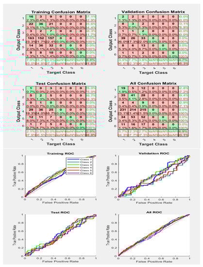
Figure 18.
Neural Network Model ROC (Receiver Operating Characteristics) and Confusion Matrix for LM TrainFcn/Activation Function at level 9 (RMS) Features for High Contact Resistance Fault with 93.1% Accuracy. Grey line shows diagonal of the ROC for indicating Class 1–6 lines are lying above or below or on it.
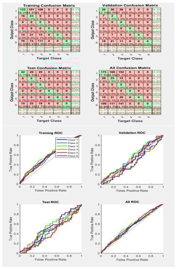
Figure 19.
Neural Network Model ROC (Receiver Operating Characteristics) and Confusion Matrix for LM TrainFcn/Activation Function at level 9 (RMS) Features for High Contact Resistance Fault with 80.0% Accuracy. Grey line shows diagonal of the ROC for indicating Class 1–6 lines are lying above or below or on it.
From the above figures, it is shown that, with 91.0% accuracy, most of the Phases are classified with good results, and in Figure 20, with am accuracy of 85.8%, some faults are incorrectly classified, with Phase lines below the diagonal line. In addition to this, the CGP training/activation function here is used to obtain results with same number of samples.
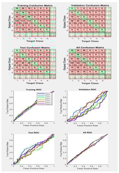
Figure 20.
Neural Network Model ROC (Receiver Operating Characteristics) and Confusion Matrix for CGP TrainFcn/Activation Function at level 9 (RMS) Features for High Contact Resistance Fault with 85.8% Accuracy. Grey line shows diagonal of the ROC for indicating Class 1–6 lines are lying above or below or on it.
The rate value of a full load current of 5.5 HP (4 kW) three-phase motor is between 8–10 A under normal working conditions. Motors typically generate 3.6 times the normal rate current under short circuit conditions. In this paper, a short circuit current of approximately (9.2 × 3.6 = 33.12 A) is obtained. The results are validated by iteration three times. In the open circuit, there is no current flow. In this case, there are no characteristic signs of motor current, as our algorithm takes a single-phase current as the input for the balanced three-phases. The high contact resistance accuracy results for RMS features are tabulated at different levels and with different accuracies, and the derived tabulated results are shown.
The ROC’s curves and confusion matrix are as shown in Figure 14, Figure 15, Figure 16, Figure 17, Figure 18, Figure 19, Figure 20 and Figure 21, accordingly. Table 3 shows 76.0%-TrainFcn = ‘oss’, 82.6%-TrainFcn = ‘oss’, 92.2%-TrainFcn = ‘oss’, 74.8%-TrainFcn = ‘lm’, 80.0%-TrainFcn = ‘lm’, 93.1%-TrainFcn = ‘lm’, 85.8%-TrainFcn = ‘cgp’ and 91.0%-TrainFcn = ‘cgp’ accuracies using different TrainFcn are obtained, respectively, for High Contact resistance faults, as presented in Table 3 for level 9 RMS features. Similarly, for the accuracies obtained from the rest of the levels, as shown in the table for RMS features of HCR Faults, or for any other type of fault at different levels for different features, we can get the ROCs and Confusion matrix results, as shown in the Figure 14 and Figure 15, and so on.
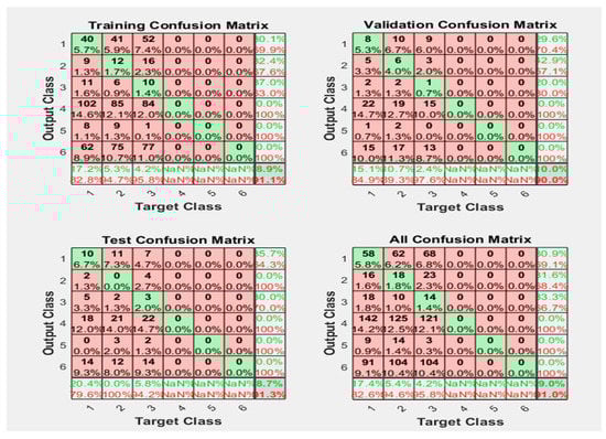
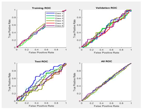
Figure 21.
Neural Network Model ROC (Receiver Operating Characteristics) and Confusion Matrix for CGP TrainFcn/Activation Function at level 9 (RMS) Features for High Contact Resistance Fault with 91.0% Accuracy. Grey line shows diagonal of the ROC for indicating Class 1–6 lines are lying above or below or on it.
Table 3.
High Contact Resistance Fault with RMS Feature Accuracies under different Activation Functions.
Figure 22, Figure 23, Figure 24, Figure 25, Figure 26 and Figure 27 have ROCs with good positive rates and all Phases with good classification, which means that good accuracy results have good ROCs with Phase lines above the grey diagonal line.
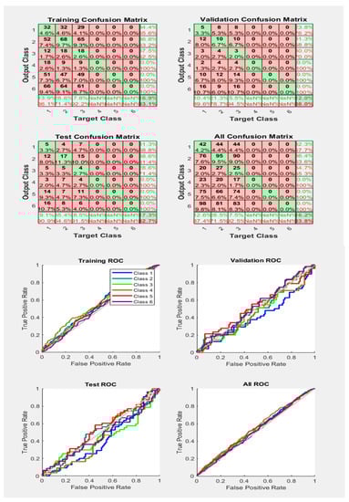
Figure 22.
Neural Network Model ROC (Receiver Operating Characteristics) and Confusion Matrix for OSS TrainFcn/Activation Function at level 9 (RMS) Features for Rotor Bar Fault with 83.8% Accuracy. Grey line shows diagonal of the ROC for indicating Class 1–6 lines are lying above or below or on it.
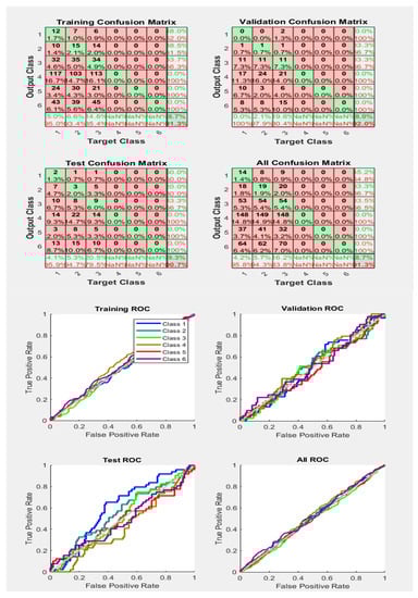
Figure 23.
Neural Network Model ROC (Receiver Operating Characteristics) and Confusion Matrix for CGP TrainFcn/Activation Function at level 9 (RMS) Features for Rotor Bar Fault with 91.3% Accuracy. Grey line shows diagonal of the ROC for indicating Class 1–6 lines are lying above or below or on it.
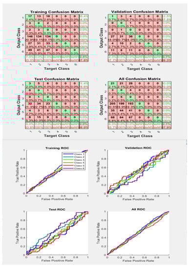
Figure 24.
Neural Network Model ROC (Receiver Operating Characteristics) and Confusion Matrix for CGP TrainFcn/Activation Function at level 9 (RMS) Features for Rotor Bar Fault with 97.9% Accuracy. Grey line shows diagonal of the ROC for indicating Class 1–6 lines are lying above or below or on it.
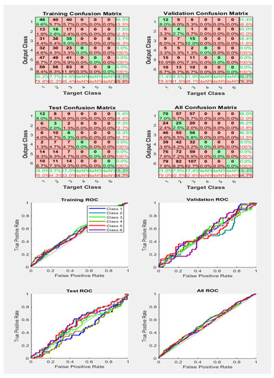
Figure 25.
Neural Network Model ROC (Receiver Operating Characteristics) and Confusion Matrix for LM TrainFcn/Activation Function at level 9 (RMS) Features for Rotor Bar Fault with 84.7% Accuracy. Grey line shows diagonal of the ROC for indicating Class 1–6 lines are lying above or below or on it.
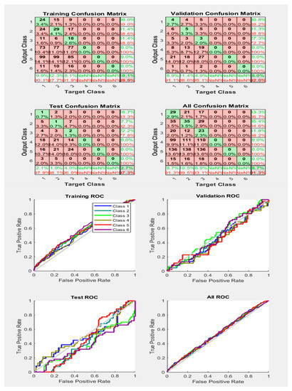
Figure 26.
Neural Network Model ROC (Receiver Operating Characteristics) and Confusion Matrix for LM TrainFcn/Activation Function at level 9 (RMS) Features for Rotor Bar Fault with 91.3% Accuracy. Grey line shows diagonal of the ROC for indicating Class 1–6 lines are lying above or below or on it.
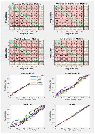
Figure 27.
Neural Network Model ROC (Receiver Operating Characteristics) and Confusion Matrix for LM TrainFcn/Activation Function at level 9 (RMS) Features for Rotor Bar Fault with 98.6% Accuracy. Grey line shows diagonal of the ROC for indicating Class 1–6 lines are lying above or below or on it.
Table 4, presents the accuracy results for rotor bar fault with RMS features at different levels, and it is concluded that ROCs curves and confusion matrix of Figure 22, Figure 23, Figure 24, Figure 25, Figure 26 and Figure 27 with accuracies and respective training functions are obtained for rotor bar fault, as shown in Table 4 for level 9 RMS features. By a similar approach, we can get the results of ROCs and confusion matrix for accuracy perspective for different faults at different levels for different features. Table 5 and Table 6 show HCR fault and Rotor Bar faults respectively with Mean features accuracies under different actions functions.
Table 4.
Rotor Bar Fault with RMS Feature Accuracies under different Activation functions.
Table 5.
High Contact Resistance Fault with Mean Feature Accuracies under different Activation Functions.
Table 6.
Rotor Bar Fault with Mean Feature Accuracies under different Activation Functions.
6. Results
The results show that different activation functions have been used to obtain greater accuracy by changing the optimizing parameters, as compared to the results obtained in [21], where it may be noted in Table 1 that 95% accuracy had been achieved using an ANN. Moreover, in this research, 96.3%, 97.1%, and 98.0% accuracy are achieved, respectively, using Trainbfg, Trainlm, and Trainoss activation functions for the HCR and rotor bar faults at different levels, specifically for the mean and RMS features. The mean features show the functioning or working features for the fault detection, as well as contain the overall important and useful information (features/data points) of the faults. Moreover, mean covers all the values of the dataset. From the Table 1 in [23], this research contributes mainly regarding two faults (high-contact resistance fault and rotor bar fault) with the implementation of an ANN classifier. Although the ANN classifier has been used with different type of faults, particularly for stator winding faults, as tabulated in Table 1 in [24] and discussed in the ‘Related Work’ section of this paper, the accuracies of fault detection and classification for the mentioned faults with different techniques are lower than the accuracies achieved in this research.
Discussion
Technically speaking, some other approaches are also recommended for detection and classification of faults for the features that are fed as an input to the system. Linear Discriminant Analysis (LDA) and Principle Component Analysis (PCA), supervised and unsupervised machine learning techniques for dimensionality reduction approaches of data, both look for linear combinations of the features which best explain the data. Furthermore, ANN as a classifier uses an iterative-based approach, and accordingly, by retraining the classifier we get higher accuracy. In that case, LDA is preferred for obtaining perfect accuracy without further iterations, and LDA is trained on the dataset one time to get good accuracy. Both LDA and PCA are recommended for future work. Moreover, the ANN approach is iterative and retrains the system several times to achieve the highest accuracy, and preferably, for good classification results. On the contrary, this is not a mechanism for the LDA and PCA classifiers.
No doubt, IoT enables the exchange of data and connection of technologies with other devices using cloud-based networks and systems over the Internet, however, the most recent advancements in technology have also supported the opportunity and facility of Mobile Edge Computing (MEC) approaches [24], which can manage the time delay and energy consumption of IoT devices more appropriately.
7. Conclusions
The results show that mean features had greater accuracy than RMS features. Furthermore, when a fault appeared, the variance in detail coefficients had increased beyond the coefficients of healthy motor signal details. Moreover, in this research, the ANN classifier was used; by retraining the classifier and optimizing the parameters, even 100% accuracy could be obtained. However, so far, an accuracy of 98.0% was achieved using mean rotor bar fault features. Table 7 shows entropy features for the rotor bar fault, and it is found that with entropy features, 0.0% accuracies are obtained. Here, an ANN classifier with 21 hidden layers and 11 epochs was trained. The results obtained are based on an iterative method, since repeatedly training the algorithm can yield more accurate results. Accordingly, the best result is considered and achieved by training the algorithm several times. As presented in the tables, different accuracies are obtained using the ANN classifier at various levels. In addition, 98.0% accuracy is obtained using mean features for the rotor bar fault at level 7, while 98.6% accuracy is obtained for rotor bar fault with RMS features at level 9. Furthermore, 96.4% accuracy was achieved for the HCR fault, and was classified using RMS features at level 5. Therefore, it may be concluded that the faults have been classified according to different features with good accuracy. Figure 13 presents the tested results for the HCR fault at level 9 with RMS features, using the ‘npr’ tool in MATLAB. Meanwhile, the ANN was trained to obtain results and for training and testing purposes. The utility of this work lies in its application in monitoring induction motors to ensure their availability in an IoT environment. Availability, as the core component of cyber-security, is the ease with which an organization’s critical data, applications, induction machines, and system resources can be accessed by authorized users in times of need.
Table 7.
Rotor Bar Fault with Entropy Features Accuracies with different Activation Functions.
Author Contributions
Conceptualization, M.Z., F.A.S. and S.K.; methodology, M.Z., F.A.S. and S.K.; software, M.Z., F.A.S., S.K. and M.I.; validation, M.Z., F.A.S., S.K., A.M.A., M.U., M.K.H. and W.T.; formal analysis, M.Z., W.T., F.A.S., S.K. and M.I.; investigation, M.Z., F.A.S. and A.M.A.; writing—original draft preparation, M.Z., F.A.S., W.T. and M.U.; writing—review and editing, M.Z., F.A.S., S.K., M.I. and A.M.A.; supervision, F.A.S., W.T., M.U. and S.K.; funding acquisition, A.M.A., M.I., S.K. and S.A. All authors have read and agreed to the published version of the manuscript.
Funding
This research received no external funding.
Institutional Review Board Statement
Not applicable.
Informed Consent Statement
Not applicable.
Data Availability Statement
Not applicable.
Acknowledgments
The researchers would like to thank the Deanship of Scientific Research Qassim University for funding the publication of this project.
Conflicts of Interest
The authors declare no conflict of interest.
Appendix A
| Definition of Parameters and Legend: Close all; Clear all; % This script assumes these variables are defined: % FeaturesRMSHealthyHCRlevel9—input data. % Output10006Inputs—target data. x = FeaturesRMSHealthyRotorlevel9; %(x is input data-trained in NN Classifier) t = Output10006Inputs; %(t represents output data) % The names can be replaced as per demand or according to the dataset names at user-side % Choose a Training Function % For a list of all training functions type: help nntrain % ‘trainlm’ is usually fastest. % ‘trainbr’ takes longer but may be better for challenging problems. % ‘trainscg’ uses less memory. Suitable in low memory situations. trainFcn = ‘trainlm’; % Scaled conjugate gradient backpropagation. %(trainFcn(Activation-Funcation)can be replaced with, i-e ‘oss’,’lm’,’cgp’ and so on) % Create a Pattern Recognition Network hiddenLayerSize = 21; net = patternnet(hiddenLayerSize, trainFcn); % Setup Division of Data for Training, Validation, Testing net.divideParam.trainRatio = 70/100; net.divideParam.valRatio = 15/100; net.divideParam.testRatio = 15/100; % Train the Network [net, tr] = train (net, x, t); % Test the Network y = net(x); e = gsubtract(t, y); performance = perform (net, t, y) tind = vec2ind (t); yind = vec2ind(y); percentErrors = sum(tind ~= yind)/numel(tind); % View the Network view(net) % Plots % Uncomment these lines to enable various plots. %figure, plotperform(tr) %figure, plottrainstate(tr) %figure, ploterrhist(e) %figure, plotconfusion(t, y) %figure, plotroc (t, y) end |
References
- Jigyasu, R.; Sharma, A.; Mathew, L.; Chatterji, S. A Review of Condition Monitoring and Fault Diagnosis Methods for Induction Motor. In Proceedings of the 2018 Second International Conference on Intelligent Computing and Control Systems (ICICCS), Madurai, India, 14–15 June 2018; pp. 1713–1721. [Google Scholar] [CrossRef]
- Reddy, B.K. Condition Monitoring and Life extension of Induction Motor. TEST Eng. Manag. 2020, 82, 8645–8651. [Google Scholar]
- Kumar, P.; Hati, A.S. Review on machine learning algorithm based fault detection in induction motors. Arch. Comput. Methods Eng. 2021, 28, 1929–1940. [Google Scholar] [CrossRef]
- Fontes, A.S.; Cardoso, C.A.; Oliveira, L.P. Comparison of techniques based on current signature analysis to fault detection and diagnosis in induction electrical motors. In Proceedings of the 2016 Electrical Engineering Conference (EECon), Colombo, Sri Lanka, 15 December 2016; p. 74. [Google Scholar]
- Deeb, M.; Kotelenets, N.F. Fault diagnosis of 3-phase induction machine using harmonic content of stator current spectrum. In Proceedings of the 2020 International Youth Conference on Radio Electronics, Electrical and Power Engineering (REEPE), Moscow, Russia, 12–14 March 2020; pp. 1–6. [Google Scholar]
- AlShorman, O.; Irfan, M.; Saad, N.; Zhen, D.; Haider, N.; Glowacz, A.; AlShorman, A. A review of artificial intelligence methods for condition monitoring and fault diagnosis of rolling element bearings for induction motor. Shock Vib. 2020, 2020, 8843759. [Google Scholar] [CrossRef]
- Deeb, M.; Kotelenets, N.F.; Assaf, T.; Sultan, H.M. Three-Phase Induction Motor Short Circuits Fault Diagnosis using MCSA and NSC. In Proceedings of the 2021 3rd International Youth Conference on Radio Electronics, Electrical and Power Engineering (REEPE), Moscow, Russia, 11–13 March 2021; pp. 1–6. [Google Scholar]
- Sridhar, S.; Rao, K.U.; Jade, S. Detection of broken rotor bar fault in induction motor at various load conditions using wavelet transforms. In Proceedings of the 2015 International Conference on Recent Developments in Control, Automation and Power Engineering (RDCAPE), Noida, India, 12–13 March 2015; pp. 77–82. [Google Scholar] [CrossRef]
- Zolfaghari, S.; Noor, S.B.; Rezazadeh Mehrjou, M.; Marhaban, M.H.; Mariun, N. Broken rotor bar fault detection and classification using wavelet packet signature analysis based on fourier transform and multi-layer perceptron neural network. Appl. Sci. 2018, 8, 25. [Google Scholar] [CrossRef]
- Maciejewski, N.A.; Treml, A.E.; Flauzino, R.A. A Systematic Review of Fault Detection and Diagnosis Methods for Induction Motors. In Proceedings of the 2020 FORTEI-International Conference on Electrical Engineering (FORTEI-ICEE), Bandung, Indonesia, 23–24 September 2020; pp. 86–90. [Google Scholar]
- Sharma, A.; Mathew, L.; Chatterji, S. Analysis of Broken Rotor bar Fault Diagnosis for Induction Motor. In Proceedings of the IEEE International Conference on Innovations in Control, Communication and Information Systems (ICICCI), Greater Noida, India, 12–13 August 2017; pp. 492–497. [Google Scholar]
- Purushottam, G.; Tiwari, R. Online diagnostics of mechanical and electrical faults in induction motor using multiclass support vector machine algorithms based on frequency domain vibration and current signals. ASCE-ASME J. Risk Uncertain. Eng. Syst. Part B Mech. Eng. 2019, 5, 031001. [Google Scholar]
- Liang, X.; Ali, M.Z.; Zhang, H. Induction Motors Fault Diagnosis Using Finite Element Method: A Review. IEEE Trans. Ind. Appl. 2020, 56, 1205–1217. [Google Scholar] [CrossRef]
- Terron-Santiago, C.; Martinez-Roman, J.; Puche-Panadero, R.; Sapena-Bano, A. A Review of Techniques Used for Induction Machine Fault Modelling. Sensors 2021, 21, 4855. [Google Scholar] [CrossRef]
- Merizalde, Y.; Hernández-Callejo, L.; Duque-Perez, O. State of the art and trends in the monitoring, detection and diagnosis of failures in electric induction motors. Energies 2017, 10, 1056. [Google Scholar] [CrossRef]
- Toma, R.N.; Prosvirin, A.E.; Kim, J.M. Bearing fault diagnosis of induction motors using a genetic algorithm and machine learning classifiers. Sensors 2020, 20, 1884. [Google Scholar] [CrossRef]
- Zamudio-Ramírez, I.; Osornio-Ríos, R.A.; Antonino-Daviu, J.A.; Quijano-Lopez, A. Smart-sensor for the automatic detection of electromechanical faults in induction motors based on the transient stray flux analysis. Sensors 2020, 20, 1477. [Google Scholar] [CrossRef]
- Adouni, A.; Marques Cardoso, A.J. Thermal analysis of low-power three-phase induction motors operating under voltage unbalance and inter-turn short circuit faults. Machines 2020, 9, 2. [Google Scholar] [CrossRef]
- Martinez-Herrera, A.L.; Ferrucho-Alvarez, E.R.; Ledesma-Carrillo, L.M.; Mata-Chavez, R.I.; Lopez-Ramirez, M.; Cabal-Yepez, E. Multiple Fault Detection in Induction Motors through Homogeneity and Kurtosis Computation. Energies 2022, 15, 1541. [Google Scholar] [CrossRef]
- Albattah, W.; Khel, M.H.K.; Habib, S.M.; Khan, S.; Kadir, K.A. Hajj Crowd Management Using CNN-Based Approach. Comput. Mater. Contin. 2020, 66, 2183–2197. [Google Scholar] [CrossRef]
- Purushottam, G.; Tiwari, R. Signal based condition monitoring techniques for fault detection and diagnosis of induction motors: A state-of-the-art review. Mech. Syst. Signal Process. 2020, 144, 106908. [Google Scholar]
- Esakimuthu Pandarakone, S.; Mizuno, Y.; Nakamura, H. A comparative study between machine learning algorithm and artificial intelligence neural network in detecting minor bearing fault of induction motors. Energies 2019, 12, 2105. [Google Scholar] [CrossRef]
- Mohamed, M.A.; Hassan, M.A.M.; Albalawi, F.; Ghoneim, S.S.M.; Ali, Z.M.; Dardeer, M. Diagnostic Modeling for Induction Motor Faults via ANFIS Algorithm and DWT-Based Feature Extraction. Appl. Sci. 2021, 11, 9115. [Google Scholar] [CrossRef]
- Cui, Y.Y.; Zhang, T. New Quantum-Genetic Based OLSR Protocol (QGOLSR) for Mobile Ad hoc Network. Appl. Soft Comput. 2019, 80, 285–296. [Google Scholar] [CrossRef]
- Zhang, T.; Zhang, D.; Qiu, J.; Zhang, X.; Zhao, P.; Gong, C. A Kind of Novel Method of Power Allocation with Limited Cross-Tier Interference for CRN. IEEE Access 2019, 7, 82571–82583. [Google Scholar] [CrossRef]
- Li, T.; Dong, Q.; Wang, Y.; Gong, X.; Yang, Y. Dual buffer rotation four-stage pipeline for CPU–GPU cooperative computing. Soft Comput. 2017, 23, 859–869. [Google Scholar] [CrossRef]
- Abid, A.; Khan, M.T.; Iqbal, J. A review on fault detection and diagnosis techniques: Basics and beyond. Artif. Intell. Rev. 2021, 54, 3639–3664. [Google Scholar] [CrossRef]
- Chen, S. Review on Supervised and Unsupervised Learning Techniques for Electrical Power Systems: Algorithms and Applications. IEEJ Trans. Electr. Electron. Eng. 2021, 16, 1487–1499. [Google Scholar] [CrossRef]
- Hsueh, Y.M.; Ittangihal, V.R.; Wu, W.B.; Chang, H.C.; Kuo, C.C. Fault diagnosis system for induction motors by CNN using empirical wavelet transform. Symmetry 2019, 11, 1212. [Google Scholar] [CrossRef]
- Valtierra-Rodriguez, M.; Rivera-Guillen, J.R.; Basurto-Hurtado, J.A.; De-Santiago-Perez, J.J.; Granados-Lieberman, D.; Amezquita-Sanchez, J.P. Convolutional neural network and motor current signature analysis during the transient state for detection of broken rotor bars in induction motors. Sensors 2020, 20, 3721. [Google Scholar] [CrossRef]
- Nishat Toma, R.; Kim, J.M. Bearing fault classification of induction motors using discrete wavelet transform and ensemble machine learning algorithms. Appl. Sci. 2020, 10, 5251. [Google Scholar] [CrossRef]
- Zhang, T.; Chen, J.; Li, F.; Zhang, K.; Lv, H.; He, S.; Xu, E. Intelligent fault diagnosis of machines with small & imbalanced data: A state-of-the-art review and possible extensions. ISA Trans. 2022, 119, 152–171. [Google Scholar]
- Tang, S.; Yuan, S.; Zhu, Y. Convolutional neural network in intelligent fault diagnosis toward rotatory machinery. IEEE Access 2020, 8, 86510–86519. [Google Scholar] [CrossRef]
- Qiao, Z.; Shu, X. Coupled neurons with multi-objective optimization benefit incipient fault identification of machinery. Chaos Solitons Fractals 2021, 145, 110813. [Google Scholar] [CrossRef]


Publisher’s Note: MDPI stays neutral with regard to jurisdictional claims in published maps and institutional affiliations. |
© 2022 by the authors. Licensee MDPI, Basel, Switzerland. This article is an open access article distributed under the terms and conditions of the Creative Commons Attribution (CC BY) license (https://creativecommons.org/licenses/by/4.0/).