Article

Non-Linear Clustering of Distribution Feeders

1
Hydro-Quebec Research Center, Varennes, QC J3X 1S1, Canada
2
Hydro-Quebec Distribution Network Strategy Unit, Montreal, QC H2Z 1A4, Canada
*
Author to whom correspondence should be addressed.
Energies 2022, 15(21), 7883; https://doi.org/10.3390/en15217883
Submission received: 16 September 2022 / Revised: 16 October 2022 / Accepted: 20 October 2022 / Published: 24 October 2022
(This article belongs to the Topic Smart Energy Systems)

Abstract

:
Distribution network planners are facing a strong shift in the way they plan and analyze the network. With their intermittent nature, the introduction of distributed energy resources (DER) calls for yearly or at least seasonal analysis, which is in contrast to the current practice of analyzing only the highest demand point of the year. It requires not only a large number of simulations but long-term simulations as well. These simulations require significant computational and human resources that not all utilities have available. This article proposes a nonlinear clustering methodology to find a handful of representative medium voltage (MV) distribution feeders for DER penetration studies. It is shown that the proposed methodology is capable of uncovering nonlinear relations between features, resulting in more consistent clusters. Obtained results are compared to the most common linear clustering algorithms.

1. Introduction

The world is seeing rapid adoption of distributed energy resources (DER) technologies; this calls for proper planning to host them in the distribution network [1,2]. Distribution network operators (DNOs) must study the impacts of a large penetration of DERs in their networks and set up mitigation measures if necessary. However, due to the sheer size of distribution networks, their numbers, and the combinatorial of DERs, an impact analysis of all technologies across all distribution feeders is a laborious process.
Identifying a set of representative feeders by grouping them in clusters of feeders with similar electrical parameters using machine learning clustering methods is of great interest for distribution network planers [2]. Having a handful of feeders representing the totality of network feeders can greatly reduce the computational and human resources needed to produce DER impact analysis. Furthermore, with proper analysis of selected cluster feeders and an overall statistical observation, the study can be scaled up across the whole network.
Applying clustering techniques to find representative distribution feeders was first introduced in [3], where the authors used the k-means (KM) algorithm to find 12 feeders that represent the whole system. The Pacific Northwest National Laboratory (PNNL) team in [4] used a different type of clustering, the hierarchical clustering algorithm (HC), to find a set of 24 medium voltage (MV) representative feeders across the USA. In [5] and [6], the authors used principal component analysis (PCA) to reduce the dimensionality of the problem. Their work resulted in 12 representative feeders for the Western USA in the first case and nine feeders in the second case. In [7], the authors performed clustering using the k-means algorithm on 8000+ distribution feeders in California. They selected 214 feeders from the resulting eight clusters and assessed their PV hosting capacity. They found that the hosting capacity for feeders within the same cluster varied widely and concluded that the clustering technique’s accuracy in predicting PV hosting capacity was low.
All of the previously mentioned approaches to cluster distribution feeders relay on linear clustering techniques such as k-means or hierarchical clustering. Even more recent clustering analyses [2,8,9,10] are not used for clustering distribution feeders but are related to distribution networks that rely on linear clustering techniques. In [2], the authors use a probabilistic approach to select attributes for density-based (DB) clustering. However, the authors do not explain how their proposed approach compares to any other clustering technique.
The disadvantage of k-means is that it is especially vulnerable to outliers. As the algorithm iterates through centroids, outliers significantly impact how the centroids move before reaching stability and convergence. Furthermore, k-means has problems accurately clustering data where the clusters are of different sizes and densities. k-means can only apply spherical clusters, and its accuracy will suffer if the data is not spherical. k-means requires us to first select the number of clusters we wish to find. On the other hand, hierarchical clustering has problems accurately clustering data where the clusters are of different sizes and densities, and clustering decisions are made arbitrarily. It works poorly with mixed data types and requires us to first select the number of clusters we wish to find.
Another issue with common clustering techniques is selecting the optimal number of clusters, which must be provided in advance. While the authors in [6] chose the optimal number of clusters based on the variance ratio criterion (VRC), they did not comment on how decisive this criterion was in determining the optimal point. In [4,5], the only method used to determine the optimal number of groups or clusters is the study of the sum of squared errors (SSE), known as the elbow criterion. While the statistics community has adopted this approach, it still lacks mathematical proof [5]. A slightly different approach is used in [11] for Australian MV feeders, where more topology-related parameters were added. The optimal number of clusters was found using the silhouette technique, which is also used in [12]. In [13], discriminant analysis techniques were used to cluster Australian feeders. All the previously mentioned work considered using only one algorithm and one criterion for finding the optimal number of clusters (elbow or silhouette). The authors in [3,4,5,6] and [14,15,16,17] used the assessment of PV hosting capacity as a validation tool for feeder clustering. While this method is efficient in interpreting the applicability of clustering, it does not help improve the clustering model. In [2,8,9,10], such criteria are not presented at all. Yet, with a variety of clustering techniques, one cannot be certain that optimal clustering is achieved since each technique has its own advantages and drawbacks. In addition, a thorough comparative analysis across different techniques is required to discover all possible structures of the data. The authors in [7] used four different algorithms as well as more features covering residential feeders’ electrical and customer characteristics; however, the comparative analysis between the algorithms was limited and consisted of only analyzing the silhouette score.
This paper describes a clustering methodology for MV distribution feeders that uses a nonlinear dimensionality-reduction technique to produce a density-based clustering. We show that the obtained clusters are more consistent than the ones obtained by linear techniques. Obtained results are compared to more common techniques such as k-means and hierarchical algorithm combined with three indicators to determine the optimal number of clusters. A unique aspect of this methodology lies in performing a comparative study across the clustering techniques to ensure that the optimal clustering is achieved, as proposed in [7]. Another aspect lies in performing a systematic validation of the clustering results, where the clustering can be transformed into an iterative process to improve the quality of clusters.

2. Clustering Analysis

Clustering is an unsupervised learning problem that aims to reveal data structure by grouping samples into classes based on their similarities [18]. In this section, the tools used in the clustering process are described.

2.1. Algorithms

A variety of clustering methods [18], such as partitioning methods, hierarchical methods, density-based methods, and distribution-based methods, are available. For this study, the following algorithms are used:
(1) k-means++ [18,19]: a partitioning method that groups the data by trying to separate the samples into n groups based on minimizing a criterion called inertia or sum of squares of the cluster criterion. This method performs well with a large number of samples; however, it starts losing efficiency when the number of clusters is high or if the clusters have nonconvex shapes.
Moreover, k-means++ begins with the random assignment of a cluster center, then searches for other centers based on the first one. This approach is more effective than the arbitrary initialization of the n centroids by the k-means algorithm, wherein converging to a local minimum is more probable.
(2) Hierarchical algorithm [18]: a hierarchical method that involves two techniques: agglomerative and divisive. The agglomeration algorithm performs a hierarchical classification using an ascending approach. Each observation starts in its own cluster, and the clusters are successively merged.
The linkage criteria for merging, Ward, minimizes the sum of squared differences in all clusters. It is an approach similar to the objective function of k-means. In order to avoid a computationally expensive problem, connectivity constraints are added to the algorithm restraining it from merging far-apart samples.
(3) DBSCAN [20]: is a density-based algorithm. This algorithm tends to group points into clusters of different densities. The algorithm is able to find clusters due to the density of points in a given area which is higher inside a cluster than outside.

2.2. Optimal Number of Clusters

The first two algorithms require the specification of an optimal number of clusters, which is one of the most important tasks for those clustering processes [16]. Therefore, three indicators are used and compared here for this task.
(1) Silhouette score [17]: one of the most used methods to determine the optimal number of clusters. It involves assigning a silhouette score (SC) ranging between −1 and 1 to each sample, where this score describes the similarity and the dissimilarity of the sample in its cluster. A higher silhouette score indicates more coherent (dense and well-separated) clusters. Similar to the inertia criterion of the k-means algorithm, the silhouette score tends to be lower for clusters with irregular shapes than for clusters with convex shapes.
(2) Variance ratio criterion [16]: Another method for finding the optimal number of clusters is the Calinski–Harabsz criterion or variance ratio criterion (VRC). It is the ratio between the within-cluster dispersion and the between-cluster dispersion. Similar to the silhouette a higher VRC score indicates more coherent clusters; however, calculating the VRC score takes less time than the silhouette score.
(3) Davies–Bouldin score [16]: The (DBS) score measure, by definition, takes into account the average similarity of each cluster with its neighboring cluster. Its formulation is a simpler version of the silhouette. It indicates the level of separation between clusters only.

3. Dataset

The dataset consisted of 14 selected electrical features for 2500+ distribution feeders from a distribution system of a utility covering a large area. Table 1 displays the features recommended by the distribution system operator, which characterize the topology and load distribution along the feeders.

4. Data Preprocessing

Before starting any analysis, a data checkup needs to be performed to make sure that there is no missing information. In our case, Figure 1 presents an analysis of missing features for all feeders, and missing features appear as white spaces on the figure. The figure indicates that 67 feeders have missing data for two features, the variance of the distance from the load to the source and the coefficient of variation of KVA consumed. Please notice that the distribution network planner provided the data and that the above-mentioned features were missed at the time.
There are several ways to tackle this issue. One is to simply drop the feeders with missing information from the analysis at the cost of losing information for the clustering analysis. The other is to perform simple imputation, which is to give the mean of the values to the missing one or perform more accurate approximations using the KNN Imputer of MissForest Imputer.

4.1. Data Imputation

K-nearest neighbors Impute (KNN-Impute) is a machine-learning-based imputation algorithm that has been successful but requires tuning of the parameter k and is additionally vulnerable to many of KNN’s weaknesses, such as being sensitive to outliers and noise [21].
MissForest is another machine learning-based data imputation algorithm that operates on the Random Forest algorithm [21]. Stekhoven and Buhlmann, creators of the algorithm, conducted a study in 2011 in which imputation methods were compared on datasets with randomly introduced missing values. MissForest outperformed all other algorithms in all metrics, including KNN-Impute, in some cases by over 50%. In this study, we use MissForest to impute the missing data.

4.2. Feature Selection

4.2.1. Feature Scaling

The next step consists of feature standardization by removing the mean and matching the variance (known as the z-score) [16]. This type of scaling is favored over the MinMax scaling [7], especially when using PCA, which reduces the dimensionality based on the variance [15].

4.2.2. Feature Correlation

After preparing the data, the feature correlation must be studied to ensure unbiased clustering. One method for determining the features to be used is the visualization of its covariance matrix. A large covariance coefficient between two features indicates that the features are highly correlated. This means that they contain information that can be predicted or represented by only one of the features. In Figure 2, a correlation (Pearson coefficient) matrix for the features is shown. Deciding on a threshold for the correlation involves visualizing the features by pair plots to verify the relationship between the different features. In our case, coefficients equal to or larger than 0.8 are considered correlated.
Figure 2 shows that features 5 and 6, 9 and 11, 9 and 13, 11 and 13, and 11 and 14 are highly correlated. Thus, we have decided to drop features 6, 11, and 13.

4.2.3. PCA

Principal component analysis, or PCA [15], is a linear feature extraction technique. It allows us to scale down the complexity of the variation in the data. This technique performs a linear mapping of the data to a lower dimensional space in such a way that the variance of the data in the low-dimensional representation is maximized. Using the eigenvectors of the covariance matrix, which points along the maximum variation in the data, a significant fraction of the variance of the original data is reconstructed. Thus, using PCA, the dimensionality of the data is reduced by taking the first components or eigenvectors. More components can be added if the variance explained ratios sum to less than 85%. Using PCA with three dimensions results in a 60% representation of our original data; we need six dimensions to represent more than 85% of the original variance. Two options are possible here, perform the clustering on the 11 dimensions dataset or on the 6 PCA dimensions data set.

5. Linear Clustering

As mentioned above, PCA, a linear feature extraction, is used to reduce the data’s complexity and perform clustering [22]. Clusters with PCA are not very well defined, and DBSCAN will have difficulty producing reliable clusters. Thus, in this section, we perform the clustering on the 11- and 6-dimensional datasets using k-means++ and Hierarchical Clustering.

Number of Clusters

Both algorithms require us to provide the number of clusters to be created. As mentioned in Section 2.2, we use the silhouette score (SC), variance ratio criterion (VRC), and Davies–Bouldin score (DBS) to evaluate the best number of clusters. Figure 3 shows the scores when KM is applied to the 6-dimensional dataset. Figure 4 shows the scores when KM is applied to the 11-dimensional dataset. Figure 5 shows the scores when hierarchical clustering is applied to the 6-dimensional dataset. Figure 6 shows the scores when hierarchical clustering is applied to the 11-dimensional dataset.
From these figures, we notice two things, much clearer results are obtained from the clustering on the 11-dimension dataset, and that VCR is not a good evaluation criterion. Focusing on the 11-dimensional results, we can see that KM, SC, and DBS scores indicate 5 and 4 as the best number of clusters. However, five seems a small number, so we looked for the next highest point being eight and nine, respectively. In the case of hierarchical clustering, these numbers are 6 for DBS and 7 for SC. Taking as reference the SC, which presents less variation, we selected the best number of clusters as being 8 for KM and 7 for HC.

6. Nonlinear Clustering

6.1. t-SNE

t-SNE is a nonlinear dimensionality reduction technique originally developed to visualize high dimensional data. It is a variation of stochastic neighbor embedding (SNE) that is much easier to optimize and produces significantly better visualizations. t-SNE converts a high-dimensional data set into a matrix of pair-wise similarities. It is capable of capturing much of the local structure of the high-dimensional data very well while also revealing global structures, such as the presence of clusters [23].
Although SNE constructs reasonably good visualizations, it is hampered by a cost function that is difficult to optimize, and a problem referred to as the ‘’crowding problem’’. The cost function used by t-SNE differs from the one used by SNE in two ways. (1) It uses a symmetrized version of the SNE cost function with simpler gradients, and (2) it uses a Student-t distribution rather than a Gaussian to compute the similarity between two points in the lower dimensional space. t-SNE employs heavy-tailed distribution in the low-dimensional space to alleviate both the crowding and the optimization problems of SNE.

6.2. DBSCAN

Using t-SNE to represent the high-dimensional data in a two dimensions plane allows utilization of the DBSCAN algorithm, which relies on a density-based notion of clusters and is designed to detect clusters of any shape [20].
KM is especially vulnerable to outliers. As the algorithm iterates through centroids, outliers have a significant impact on the way the centroids move before reaching stability and convergence. Furthermore, KM has problems accurately clustering data where the clusters are of different sizes and densities. KM can only apply spherical clusters, and its accuracy will suffer if the data is not spherical. KM requires us to first select the number of clusters we wish to find. On the other hand, DBSCAN does not require us to specify the number of clusters, avoids outliers, and works quite well with arbitrarily shaped and sized clusters. It does not have centroids. The clusters are formed by process of linking neighbor points together. However, it requires determining the epsilon value and the minimal number of points.

6.2.1. Optimal Parameters

In order to obtain the best epsilon and point numbers combination, we perform the clustering analysis for a set of combinations of these two parameters. We then evaluate the clustering performance by two measures, the silhouette score, which must be as high as possible, and the number of non-clustered points, which must be as low as possible. We also try to target a coherent number of clusters. If the epsilon chosen is too small, a large part of the data will not be clustered, whereas a high epsilon value cluster will merge, and most data points will be in the same cluster. In general, small values of epsilon are preferable, and as a rule of thumb, only a small fraction of points should be within this distance of each other.

6.2.2. Clustering Evaluation

As mentioned above, clustering is performed for a large set of combinations of parameters, and clustering performance is evaluated in the following parameters:
Silhouette method: a higher silhouette score is desired.
Non-clustered points: a low number of points is desired.
Obtained number of clusters: must be coherent with results for KM and HC.
Visual cluster interpretation: Once clusters are obtained, each cluster is interpreted visually. The clearer and more distinct each cluster is, the better.
Table 2 shows the results obtained with different parameters. From the table snippet, it is possible to see that the combination eps = 3.2 and Min points = 7 results in the highest silhouette score and a low number of non-clustered points for all results presenting six clusters or more. The selected combination results in seven clusters and 25 non-clustered points. Non-clustered points are manually assigned to their closest cluster.

7. Obtained Clusters

Table 3 shows the number of elements in each cluster and their classification as obtained with each of the algorithms used here. The classification of clusters is performed based on the easily spotted characteristics of elements forming a cluster. Industrial, residential, and commercial labels are given regarding the load composition. Urban and rural labels are given regarding the length of lines and cables composing the feeder; urban stands for short lines, and rural for long lines.

Comparison

Figure 7 presents the obtained clusters with DBSCAN, where a clear separation of clusters can be made. A comparison between Figure 8 and Figure 9, which present clusters obtained with KM and HC, shows that cluster separation is not clear for these methodologies.
Figure 10 presents a further inspection of elements in cluster 3. All four presented elements are classified as Urban industrial by DBSCAN. However, KM and HC classified the first two elements as belonging to cluster 3 and the last two as pertaining to cluster 7.

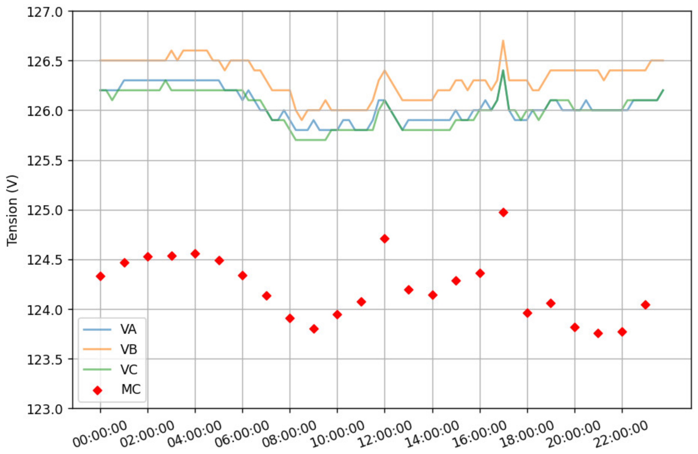
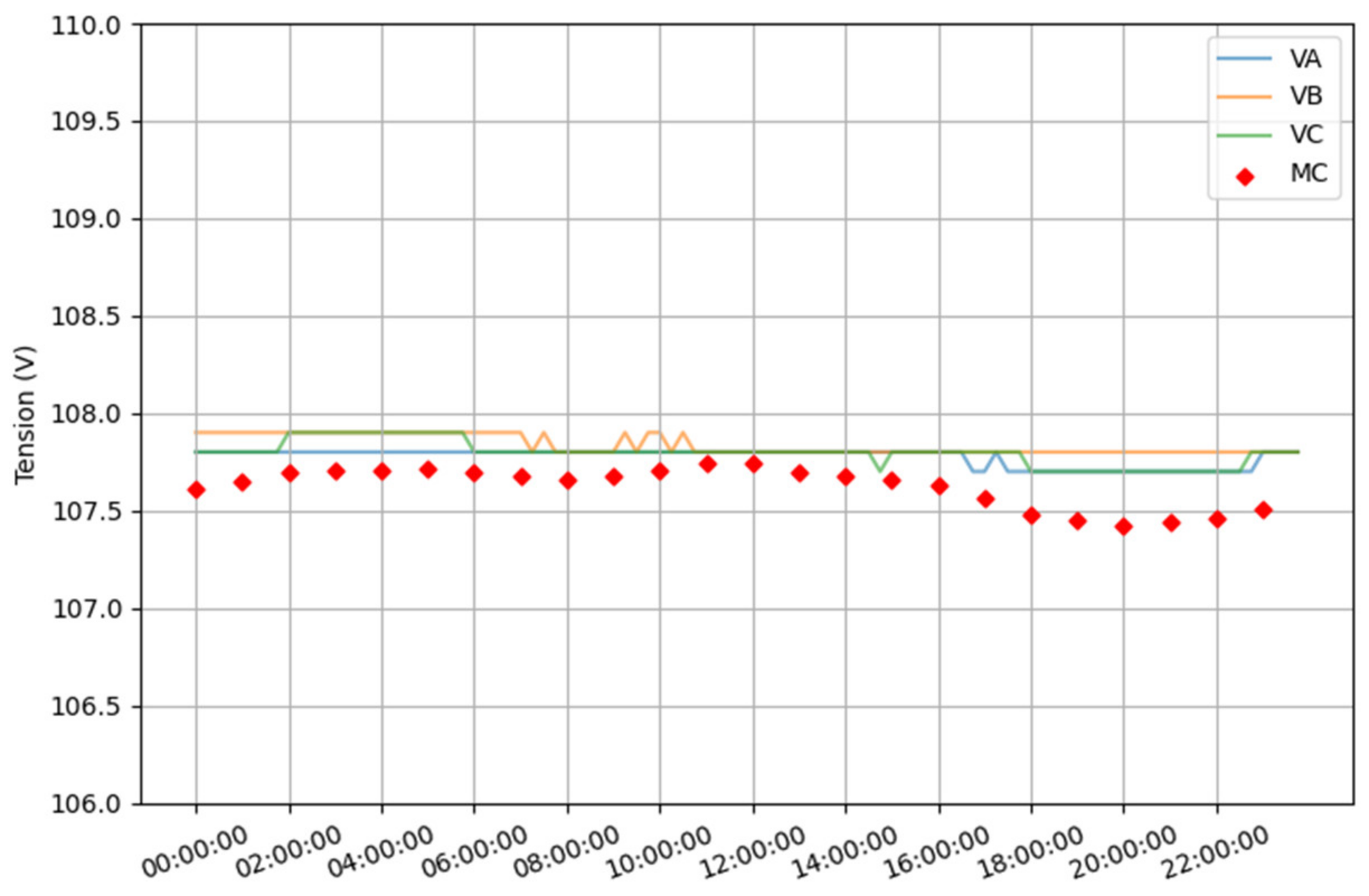
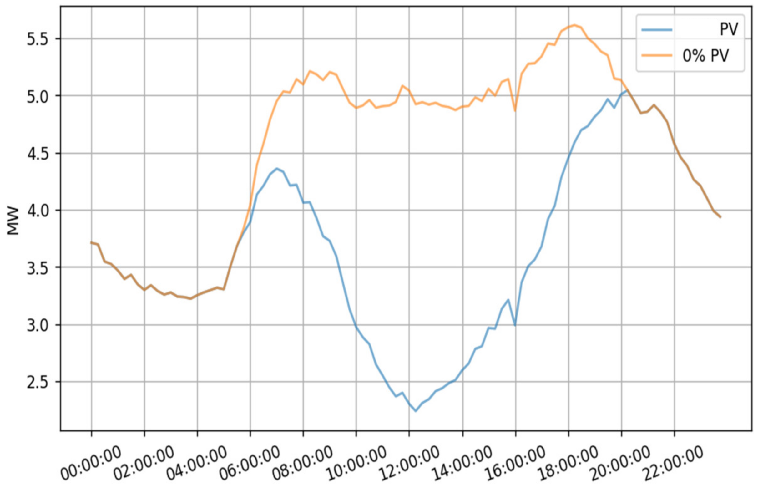
8. DER Penetration Studies

Once clusters are obtained, the next step is to validate the pertinence of inferring studies results from one feeder to another of the same cluster. A cluster may contain feeders from the same substation, which may not present many problems. But what about feeders from faraway substations?
To conduct a brief example, we have selected feeders A, B, and C from cluster 3. These feeders are close to coordinates (30,−20), (10,30), (50,−40) in Figure 7, respectively. Feeders A and B are geographically located more than 1 000 km apart from one another. For comparison, feeder D, which pertains to cluster 1 and is located 50 km away from feeder A has also been selected.
In the example, feeder and load voltages are measured before and after introducing 2.7 MW of PV production. The transformer’s tap changers are deactivated to observe the voltage’s natural behavior. Daily load and PV production profiles are for the summer period when feeders consume the least amount of power and PV installations have the largest production.
Figure 11, Figure 12, Figure 13 and Figure 14 show voltages at the substation level as well as the average of all load voltages for feeders A, B, C, and D before introducing PV production, respectively. From these figures, it can be seen that feeder voltages are inside a 0.5 V, 1 V, and 1 V window for feeders A, B, and C. Whereas for feeder D, these voltages are inside a 0.2 V window. The maximum average load voltage drop is 2 V, 3 V, and 2.5 V for feeders A, B, and C that belong to the same cluster. For feeder D, which belongs to cluster 1, the maximum average voltage drop is 0.3 V.
Figure 15, Figure 16, Figure 17 and Figure 18 show feeder voltages as well as the average of all load voltages when 2.7 MW of uniformly distributed PV production is introduced in the feeder. From these figures, it can be noticed that feeder voltages increased by up to 0.3 V, 0.5 V, 0.4 V, and 0.1 V for feeders A, B, C, and D, respectively. Average load voltages increased by up to 1.4 V, 1.1 V, 1.1 V, and 0.3 V for feeders A, B, C, and D.
Figure 19, Figure 20, Figure 21 and Figure 22 compare the active power before and after introducing 2.7 MW of PV production in feeders A, B, C, and D, respectively. These figures show that PV production causes feeders A, B, and C to be at 0.8 MW, 2.4 MW, and 3.5 MW of power flow inversion. Whereas for feeder D, it will cause power flow inversion.
Figure 23, Figure 24, Figure 25 and Figure 26 compare the reactive power before and after introducing 2.7 MW of PV production in feeders A, B, C, and D, respectively. From these figures, it can be noticed that PV production causes a reduction of reactive power consumption of 0.15 MVAR, 0.15 MVAR, 0.12 MVAR, and 0.04 MVAR.
These results show that the feeders that belong to the same cluster present similar results, whereas the elements that do not belong to the cluster present clearly different results. Thus, several conclusions can be made for all feeders in a cluster from one of its elements, such as the expected range of voltage drop, voltage gain in the presence of PV production, and the possibility of power flow inversion.

9. Conclusions

This paper has analyzed electrical and geographical data of 2500+ MV feeders. The nonlinear dimensionality reduction technique t-SNE, capable of uncovering nonlinear relations between features, has been used alongside DBSCAN, a density-based clustering technique, to group the 2500+ feeders in clusters of feeders that share similar characteristics. This approach has successfully identified a cluster for each feeder.
Obtained results have been compared to more common clustering techniques such as k-means and hierarchical clustering and have found that the proposed method presents more consistent clusters. We have compared three different methods to obtain the best number of clusters. We have found that SC and DBS are good indicators and that these can be used as good starting points for the nonlinear clustering method, while the VRC score performs poorly, and its use is not recommended.
The results of the DBSCAN methodology were validated in terms of topology, load demand, and voltage profiles by the network planners. In order to assess the usefulness of the clusters, a PV penetration study has been conducted using feeders from the same cluster and feeders from another cluster and analyzing their resulting active and reactive power and voltage profiles. The obtained results showed that feeders from the same cluster behave similarly compared to feeders from another cluster. This study also showed that the majority of conclusions that can be made from analyzing a single feeder of a cluster are more qualitative than quantitative. However, these conclusions are still helpful to distribution network planners.
The partitioning of the distribution network in a handful of representative feeders can help reduce the amount of time and resources needed to perform DER integration studies, as conclusions obtained for a single feeder can be transposed to hundreds of feeders. The results obtained in this article are proof of this and are encouraging for distribution network planners looking to produce DER penetration analysis.

Author Contributions

Conceptualization, O.R.-L., J.J. and B.F.; methodology, O.R.-L. and J.J.; software, O.R.-L. and J.J.; validation, O.R.-L. and B.F.; formal analysis, O.R.-L. and J.J.; investigation, O.R.-L. and J.J.; resources, B.F.; data curation, J.J.; writing—original draft preparation, O.R.-L.; writing—review and editing, B.F. and J.J.; visualization, O.R.-L.; supervision, O.R.-L. All authors have read and agreed to the published version of the manuscript.

Funding

This research received no external funding.

Data Availability Statement

Data used for the study is not publicly available.

Acknowledgments

The authors would like to acknowledge the support provided by Hydro-Quebec and the Hydro-Quebec Research Center.

Conflicts of Interest

The authors declare no conflict of interest.

References

  1. Kroposki, B. Summarizing the Technical Challenges of High Levels of Inverter Based Resources in Power Grids. In Proceedings of the Grid-Forming Inverters for Low-Inertia Power Systems Workshop, Washington, DC, USA, 20–22 April 2019. [Google Scholar]
  2. Oladeji, I.; Makolo, P.; Zamora, R.; Lie, T.T. Density-based clustering and probabilistic classification for integrated transmission-distribution network security state prediction. Electr. Power Syst. Res. 2022, 211, 108164. [Google Scholar] [CrossRef]
  3. Willis, H.L.; Tram, H.N.; Powell, R.W. A Computerized, Cluster Based Method of Building Representative Models of Distribution Systems. IEEE Trans. Power Appar. Syst. 1985, 104, 3469–3474. [Google Scholar] [CrossRef]
  4. Schneider, L.P.; Chen, Y.; Engle, D.; Chassin, D. A Taxonomy of North American Radial Distribution Feeders. In Proceedings of the IEEE Power and Energy Society General Meeting, Calgary, AB, Canada, 26–30 July 2009. [Google Scholar]
  5. Broderick, R.J.; Williams, J.R. Clustering Methodology for Classifying Distribution Feeders. In Proceedings of the IEEE 39th Photovoltaic Specialists Conference (PVSC), Tampa, FL, USA, 16–21 June 2013. [Google Scholar]
  6. Cale, J.; Palmintier, B.; Narang, D.; Carroll, K. Clustering Distribution Feeders in the Arizona Public Service Territory. In Proceedings of the 2014 IEEE 40th Photovoltaic Specialist Conference (PVSC), Denver, CO, USA, 8–13 June 2014. [Google Scholar]
  7. Broderick, R.; Munoz-Ramos, K.; Reno, M. Accuracy of Clustering as a Method to Group Distribution Feeders by PV Hosting Capacity. In Proceedings of the 2016 IEEE/PES Transmission and Distribution Conference and Exposition (T&D), Dallas, TX, USA, 3–5 May 2016. [Google Scholar]
  8. Zhang, Y.; Zhong, X.; Wang, L.; Liu, W.; Zhu, K.; Yan, L. Multi-objective Cluster Partition Method for Distribution Network Considering Uncertainties of Distributed Generations and Loads. In Proceedings of the 2022 Power System and Green Energy Conference (PSGEC), Shanghai, China, 25–27 August 2022; pp. 926–932. [Google Scholar] [CrossRef]
  9. Zhang, L.; Li, G.; Huang, Y.; Jiang, J.; Bie, Z.; Li, X.; Ling, Y.; Tian, H. Distributed Baseline Load Estimation for Load Aggregators Based on Joint FCM Clustering. IEEE Trans. Ind. Appl. 2022. [Google Scholar] [CrossRef]
  10. Malatesta, T.; Breadsell, J.K. Identifying Home System of Practices for Energy Use with K-Means Clustering Techniques. Sustainability 2022, 14, 9017. [Google Scholar] [CrossRef]
  11. Berry, A.M.; Moore, T.; Ward, J.K.; Lindsay, S.A.; Proctor, K. National Feeder Taxonomy Describing a Representative Feeder Set for Australian Networks; The Commonwealth Scientific and Industrial Research Organisation (CSIRO): Canberra, Australia, 2013. [Google Scholar]
  12. Jain, A.K.; Mather, B. Clustering Methods and Validation of Representative Distribution Feeders. In Proceedings of the 2018 IEEE/PES Transmission and Distribution Conference and Exposition, Denver, CO, USA, 16–19 April 2018. [Google Scholar]
  13. Li, Y.; Wolfs, P. Statistical Discriminant Analysis of High Voltage Feeders in Western Australia Distribution Networks. In Proceedings of the Power and Engineering Society General Meeting, Detroit, MI, USA, 24–28 July 2011. [Google Scholar]
  14. Rigoni, V.; Ochoa, L.F.; Chicco, G.; Navarro-Espinosa, A.; Gozel, T. Representative Residential LV feeders: A case study for the North West of England. IEEE Trans. Power Syst. 2016, 31, 348–360. [Google Scholar] [CrossRef]
  15. Jolliffe, I.T. Principle Component Analysis; Springer: New York, NY, USA, 2002. [Google Scholar]
  16. Milligan, G.W.; Cooper, M.C. An examination of procedures for determining the number of clusters in a data set. Psychometrika 1985, 50, 159179. [Google Scholar] [CrossRef]
  17. Rousseuw, P.J. Silhouettes: A graphical aid to the interpretation and validation of cluster analysis. J. Comput. Appl. Math. 1987, 20, 53–65. [Google Scholar] [CrossRef] [Green Version]
  18. Jain, A.K.; Dubes, R.C. Algorithms for Clustering Data; Prentice-Hall: Englewood Cliffs, NJ, USA, 1988. [Google Scholar]
  19. Pedregosa, F.; Varoquaux, G.; Gramfort, A.; Michel, V.; Thirion, B.; Grisel, O.; Blondel, M.; Prettenhofer, P.; Weiss, R.; Dubourg, V.; et al. Scikit-learn: Machine Learning in Python. J. Mach. Learn. Res. 2011, 12, 2825–2830. [Google Scholar]
  20. Schubert, E.; Sander, J.; Ester, M.; Kriegel, H.P.; Xu, X. DBSCAN revisited, revisited: Why and how you should (still) use DBSCAN. ACM Trans. Database Syst. TODS 2017, 42, 1–21. [Google Scholar] [CrossRef]
  21. Madhu, G.; Bharadwaj, B.L.; Nagachandrika, G.; Vardhan, K.S. A Novel Algorithm for Missing Data Imputation on Machine Learning. In Proceedings of the 2019 International Conference on Smart Systems and Inventive Technology (ICSSIT), Tirunelveli, India, 27–29 November 2019; pp. 173–177. [Google Scholar] [CrossRef]
  22. Ding, C. K-Means Clustering via Principal Component Analysis; Lawrence Berkeley National Laboratory: Berkeley, CA, USA, 2004.
  23. Pal, K.; Sharma, M. Performance Evaluation of Non-Linear Techniques UMAP and t-SNE For Data in Higher Dimensional Topological Space. In Proceedings of the 2020 Fourth International Conference on I-SMAC (IoT in Social, Mobile, Analytics and Cloud) (I-SMAC), Palladam, India, 7–9 October 2020; pp. 1106–1110. [Google Scholar] [CrossRef]
Figure 1. Feeders missing features.
Energies 15 07883 g001
Figure 2. Features correlation matrix.
Energies 15 07883 g002
Figure 3. Evaluation of the number of clusters when KM is applied to the 6-dimensional dataset.
Energies 15 07883 g003
Figure 4. Evaluation of the number of clusters when KM is applied to the 11-dimensional dataset.
Energies 15 07883 g004
Figure 5. Evaluation of the number of clusters when HC is applied to the 6-dimensional dataset.
Energies 15 07883 g005
Figure 6. Evaluation of the number of clusters when HC is applied to the 11-dimensional dataset.
Energies 15 07883 g006
Figure 7. Clusters obtained with the DBSCAN algorithm.
Energies 15 07883 g007
Figure 8. Clusters obtained with the KM algorithm.
Energies 15 07883 g008
Figure 9. Clusters obtained with the HC algorithm.
Energies 15 07883 g009
Figure 10. Features for some feeders of DBSCAN cluster 3.
Energies 15 07883 g010
Figure 11. Feeder voltage and the average of all load voltages of feeder A.
Energies 15 07883 g011
Figure 12. Feeder voltage and the average of all load voltages of feeder B.
Energies 15 07883 g012
Figure 13. Feeder voltage and the average of all load voltages of feeder C.
Energies 15 07883 g013
Figure 14. Feeder voltage and the average of all load voltages of feeder D.
Energies 15 07883 g014
Figure 15. Feeder voltage and the average of all load voltages of feeder A after the introduction of 2.7 MW of PV production.
Energies 15 07883 g015
Figure 16. Feeder voltage and the average of all load voltages of feeder B after the introduction of 2.7 MW of PV production.
Energies 15 07883 g016
Figure 17. Feeder voltage and the average of all load voltages of feeder C after the introduction of 2.7 MW of PV production.
Energies 15 07883 g017
Figure 18. Feeder voltage and the average of all load voltages of feeder D after the introduction of 2.7 MW of PV production.
Energies 15 07883 g018
Figure 19. Feeder A active power, before and after the introduction of 2.7 MW of PV production.
Energies 15 07883 g019
Figure 20. Feeder B active power, before and after the introduction of 2.7 MW of PV production.
Energies 15 07883 g020
Figure 21. Feeder C active power, before and after the introduction of 2.7 MW of PV production.
Energies 15 07883 g021
Figure 22. Feeder D active power, before and after the introduction of 2.7 MW of PV production.
Energies 15 07883 g022
Figure 23. Feeder A reactive power, before and after the introduction of 2.7 MW of PV production.
Energies 15 07883 g023
Figure 24. Feeder B reactive power, before and after the introduction of 2.7 MW of PV production.
Energies 15 07883 g024
Figure 25. Feeder C reactive power, before and after the introduction of 2.7 MW of PV production.
Energies 15 07883 g025
Figure 26. Feeder D reactive power, before and after the introduction of 2.7 MW of PV production.
Energies 15 07883 g026
Table 1. Selected Features.
No.Feature
1Max KVA consumed
2% of KVA residential
3% of KVA commercial
4% of KVA industrial
5Avg KVA consumed
6KVA coefficient of var
7Impedance
83 phase branches
9Total length of 1 ph overhead lines
10Total length of 1 ph underground lines
11Total length of 3 ph overhead lines
12Total length of 3 ph underground lines
13Avg. distance load-source
14Load-source coefficient of var
Table 2. Search of optimal parameters for DBSCAN clustering.
IterationNo. ClustersSCepsMinimum PointsNoise
305−0.4216243.1311
313−0.2825373.1417
325−0.1267183.1522
336−0.2608163.1626
349−0.2427053.1732
3511−0.2804203.1855
365−0.4167173.2310
373−0.2754973.2416
384−0.1118593.2521
395−0.2581293.2623
407−0.2016803.2725
4110−0.2704713.2841
425−0.4167173.3310
433−0.2754973.3416
443−0.2825843.3517
454−0.1110903.3621
465−0.1260713.3722
474−0.0583773.3832
484−0.3491033.438
493−0.2716633.4412
503−0.2713773.4514
514−0.1088713.4619
525−0.1170873.4719
534−0.0416923.4827
544−0.3623753.537
553−0.2733343.5410
563−0.2688793.5511
574−0.0770553.5615
585−0.0877803.5715
594−0.0263813.5824
Table 3. Clusters classification and the number of elements.
Cluster No.TypeNo. Elem. DBSCANNo. Elem.
HC
No. Elem. KM+
1Urban commercial/residential160513141013
2Rural residential603387420
3Urban industrial235213176
4Urban residential3215278
5Rural commercial24214110
6Urban residential/undg6211189
7Rural industrial72128
8Other 425
Publisher’s Note: MDPI stays neutral with regard to jurisdictional claims in published maps and institutional affiliations.

