
Non-Intrusive Load Monitoring Based on Swin-Transformer with Adaptive Scaling Recurrence Plot


Abstract
1. Introduction
- (1)
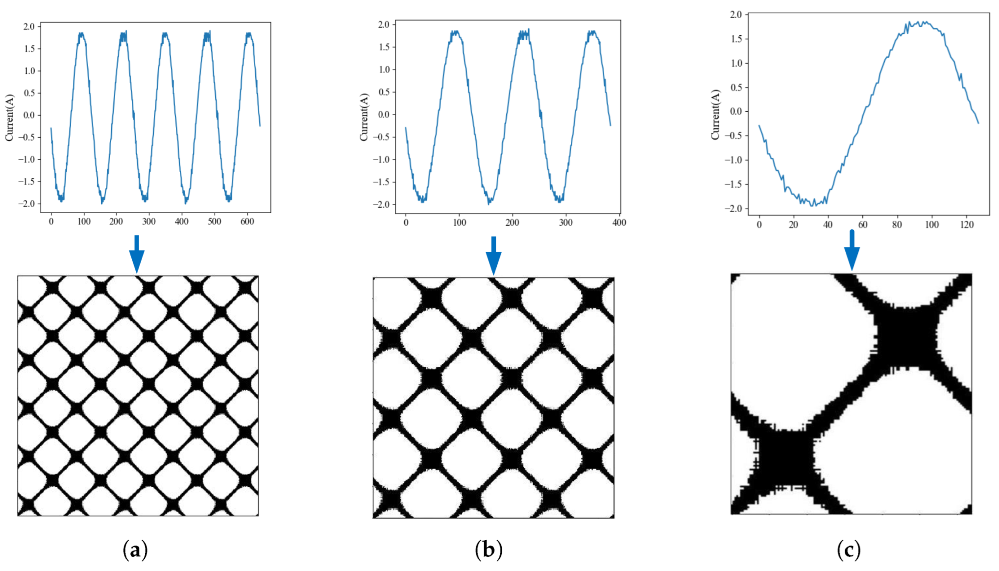
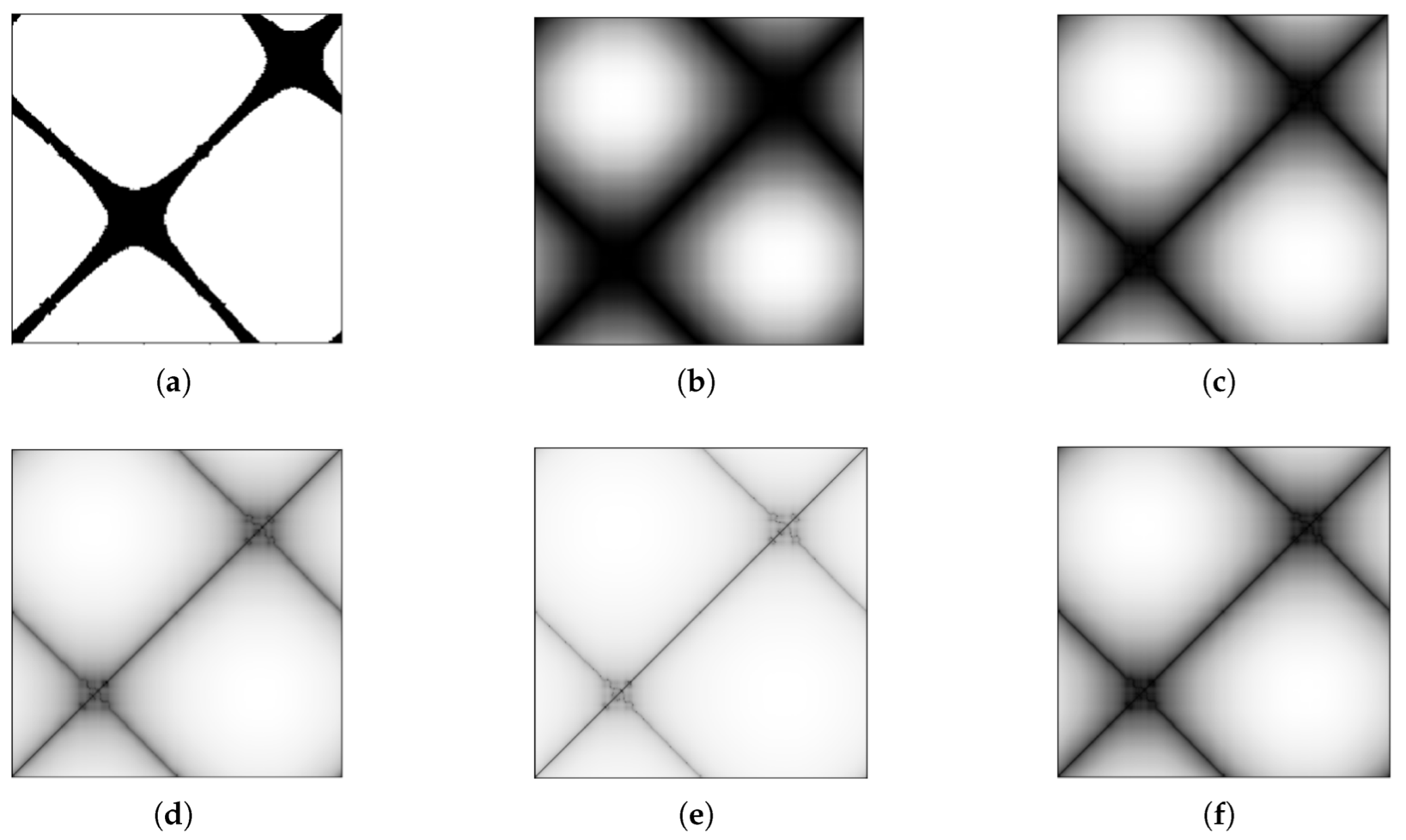
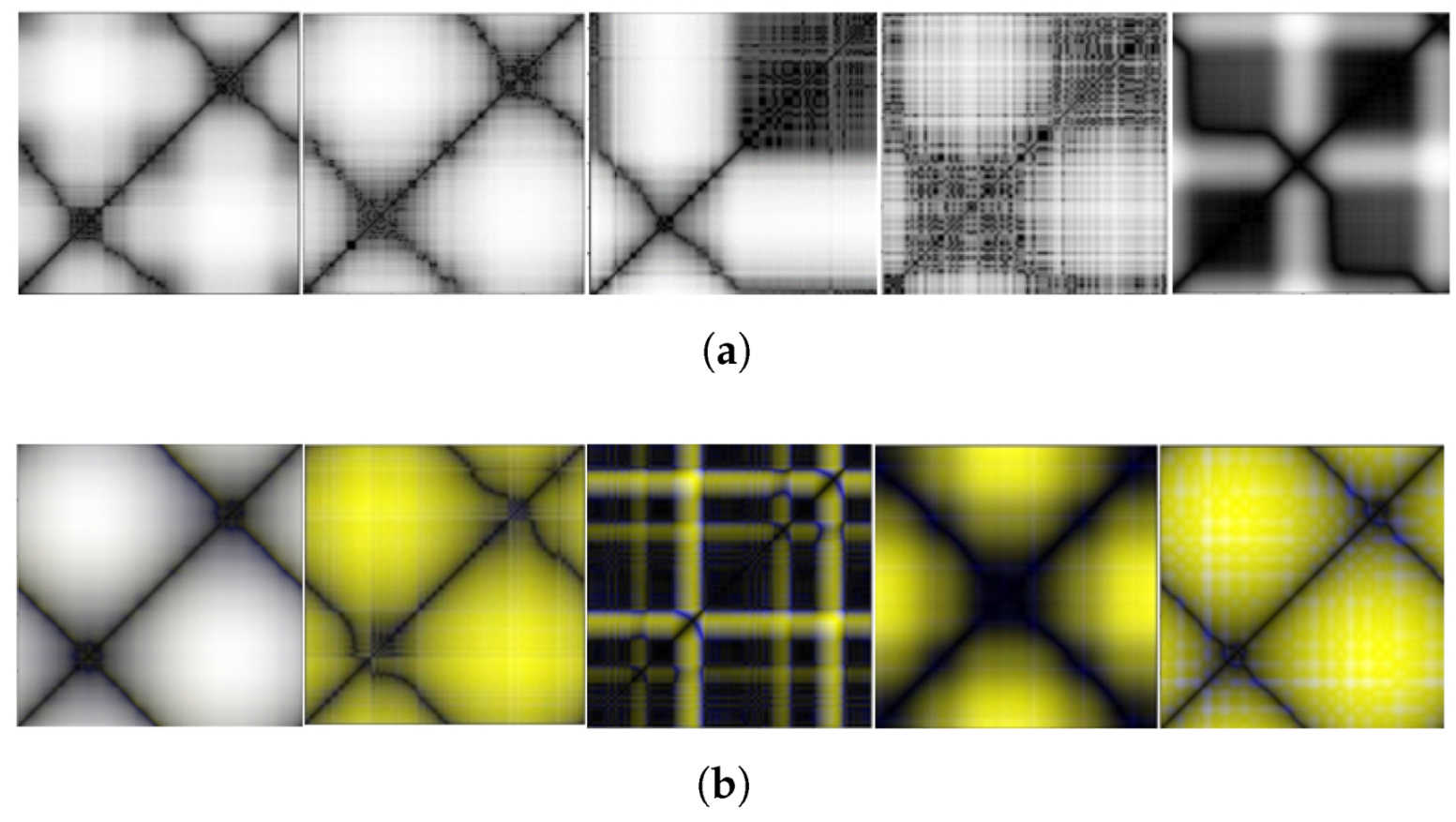
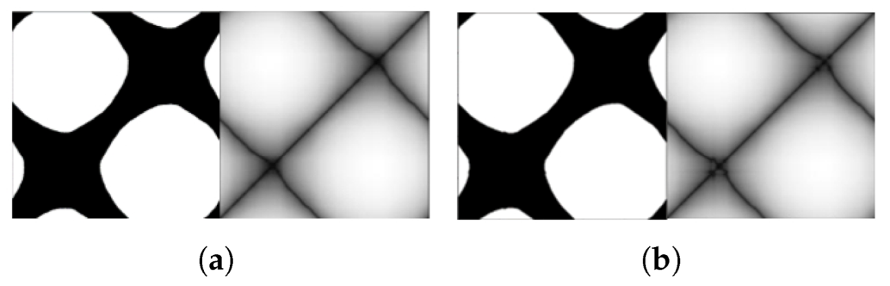
- An adaptive scaling RP (ASRP) is realized by transforming the current signal into a threshold-free RP in phase space and scaling it exponentially according to the correlation between voltage and current, which effectively reflects the working characteristics of different loads.
- (2)
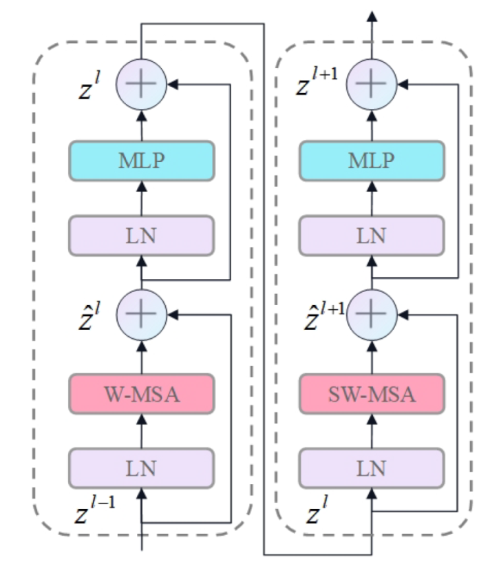
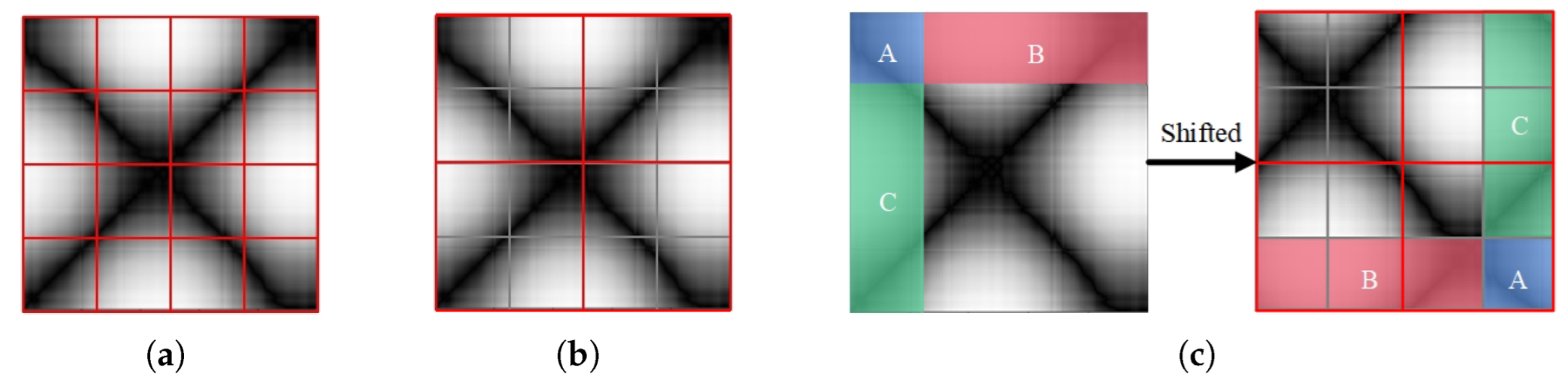
- Swin-Transformer is utilized to efficiently characterize the high-dimensional latent information in adaptive RP. In addition, the shifted window mechanism in the network can lower the computational complexity of the model. Eventually, efficient and accurate non-intrusive load identification is attained.
- (3)
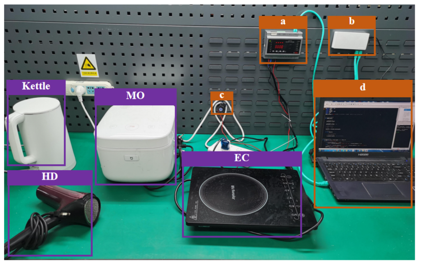
- Four measured load signal datasets, covering industrial and domestic electricity scenarios, including single-phase and three-phase electrical signals, are utilized to verify the generalizability of the proposed method.
2. Load Identification Based on Adaptive Scaling Recurrence Plot
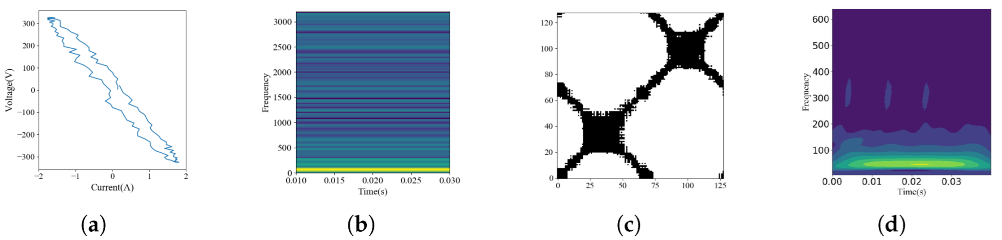
2.1. Electric Signal Preprocessing
2.2. Load Feature Extraction
| Algorithm 1 Load feature extraction based on ASRP |
| Input: is current and voltage dataset after preprocessing, D is the total number of dataset. |
| repeat |
| Update |
| Update |
| Update |
| until |
| Output: , k represents the electrical signal of the k-th phase in the dataset (single-phase: ; three-phase: ). |
2.3. Load Identification Based on Swin-Transformer
3. Experimental Design
3.1. Datasets
3.2. Method Comparison and Parameter Settings
3.3. Performance Metrics
4. Result and Discussion
5. Conclusions
Author Contributions
Funding
Data Availability Statement
Conflicts of Interest
References
- Angelis, G.F.; Timplalexis, C.; Krinidis, S.; Ioannidis, D.; Tzovaras, D. NILM applications: Literature review of learning approaches, recent developments and challenges. Energy Build. 2022, 261, 111951. [Google Scholar] [CrossRef]
- Batra, N. Systems and Analytical Techniques towards Practical Energy Breakdowns for Homes. Ph.D. Thesis, Indraprastha Institute of Information Technology, Delhi (IIIT-Delhi), Delhi, India, 2017. [Google Scholar]
- He, K.; Stankovic, L.; Liao, J.; Stankovic, V. Non-Intrusive Load Disaggregation Using Graph Signal Processing. IEEE Trans. Smart Grid 2018, 9, 1739–1747. [Google Scholar] [CrossRef]
- Carrie Armel, K.; Gupta, A.; Shrimali, G.; Albert, A. Is disaggregation the holy grail of energy efficiency? The case of electricity. Energy Policy 2013, 52, 213–234. [Google Scholar] [CrossRef]
- Athanasiadis, C.; Doukas, D.; Papadopoulos, T.; Chrysopoulos, A. A Scalable Real-Time Non-Intrusive Load Monitoring System for the Estimation of Household Appliance Power Consumption. Energies 2021, 14, 767. [Google Scholar] [CrossRef]
- Gopinath, R.; Kumar, M.; Prakash Chandra Joshua, C.; Srinivas, K. Energy management using non-intrusive load monitoring techniques – State-of-the-art and future research directions. Sustain. Cities Soc. 2020, 62, 102411. [Google Scholar] [CrossRef]
- Lin, J.; Luan, W.; Liu, B. A Novel Non-intrusive Arc Fault Detection Method for Low-Voltage Customers. In Proceedings of the 2021 6th Asia Conference on Power and Electrical Engineering (ACPEE), Chongqing, China, 8–11 April 2021; pp. 84–88. [Google Scholar] [CrossRef]
- Hart, G. Nonintrusive appliance load monitoring. Proc. IEEE 1992, 80, 1870–1891. [Google Scholar] [CrossRef]
- de Aguiar, E.L.; Lazzaretti, A.E.; Mulinari, B.M.; Pipa, D.R. Scattering Transform for Classification in Non-Intrusive Load Monitoring. Energies 2021, 14, 6796. [Google Scholar] [CrossRef]
- Mariscotti, A. Non-Intrusive Load Monitoring Applied to AC Railways. Energies 2022, 15, 4141. [Google Scholar] [CrossRef]
- Jia, D.; Li, Y.; Du, Z.; Xu, J.; Yin, B. Non-Intrusive Load Identification Using Reconstructed Voltage–Current Images. IEEE Access 2021, 9, 77349–77358. [Google Scholar] [CrossRef]
- Wang, S.; Chen, H.; Guo, L.; Xu, D. Non-intrusive load identification based on the improved voltage-current trajectory with discrete color encoding background and deep-forest classifier. Energy Build. 2021, 244, 111043. [Google Scholar] [CrossRef]
- Yang, C.C.; Soh, C.S.; Yap, V.V. A systematic approach in load disaggregation utilizing a multi-stage classification algorithm for consumer electrical appliances classification. Front. Energy 2019, 13, 386–398. [Google Scholar] [CrossRef]
- Himeur, Y.; Alsalemi, A.; Bensaali, F.; Amira, A. Effective non-intrusive load monitoring of buildings based on a novel multi-descriptor fusion with dimensionality reduction. Appl. Energy 2020, 279, 115872. [Google Scholar] [CrossRef]
- Chaurasiya, H. Time-Frequency Representations: Spectrogram, Cochleogram and Correlogram. Procedia Comput. Sci. 2020, 167, 1901–1910. [Google Scholar] [CrossRef]
- Duarte, C.; Delmar, P.; Goossen, K.W.; Barner, K.; Gomez-Luna, E. Non-intrusive load monitoring based on switching voltage transients and wavelet transforms. In Proceedings of the 2012 Future of Instrumentation International Workshop (FIIW) Proceedings, Gatlinburg, TN, USA, 8–9 October 2012; pp. 1–4. [Google Scholar] [CrossRef]
- Wenninger, M.; Bayerl, S.P.; Maier, A.; Schmidt, J. Recurrence Plot Spacial Pyramid Pooling Network for Appliance Identification in Non-Intrusive Load Monitoring. In Proceedings of the 2021 20th IEEE International Conference on Machine Learning and Applications (ICMLA), Pasadena, CA, USA, 13–16 December 2021; pp. 108–115. [Google Scholar] [CrossRef]
- Faustine, A.; Pereira, L. Improved Appliance Classification in Non-Intrusive Load Monitoring Using Weighted Recurrence Graph and Convolutional Neural Networks. Energies 2020, 13, 3374. [Google Scholar] [CrossRef]
- Bouhouras, A.S.; Gkaidatzis, P.A.; Panagiotou, E.; Poulakis, N.; Christoforidis, G.C. A NILM algorithm with enhanced disaggregation scheme under harmonic current vectors. Energy Build. 2019, 183, 392–407. [Google Scholar] [CrossRef]
- Yan, L.; Sheikholeslami, M.; Gong, W.; Tian, W.; Li, Z. Challenges for real-world applications of nonintrusive load monitoring and opportunities for machine learning approaches. Electr. J. 2022, 35, 107136. [Google Scholar] [CrossRef]
- Berrettoni, G.; Bourelly, C.; Capriglione, D.; Ferrigno, L.; Miele, G. Preliminary Sensitivity Analysis of Combinatorial Optimization (CO) for NILM Applications: Effect of the Meter Accuracy. In Proceedings of the 2021 IEEE 6th International Forum on Research and Technology for Society and Industry (RTSI), Naples, Italy, 6–9 September 2021; pp. 486–490. [Google Scholar] [CrossRef]
- Guo, Y.; Xiong, X.; Fu, Q.; Xu, L.; Jing, S. Research on non-intrusive load disaggregation method based on multi-model combination. Electr. Power Syst. Res. 2021, 200, 107472. [Google Scholar] [CrossRef]
- Gurbuz, F.B.; Bayindir, R.; Vadi, S. Comprehensive Non-Intrusive Load Monitoring Process: Device Event Detection, Device Feature Extraction and Device Identification Using KNN, Random Forest and Decision Tree. In Proceedings of the 2021 10th International Conference on Renewable Energy Research and Application (ICRERA), Istanbul, Turkey, 26–29 September 2021; pp. 447–452. [Google Scholar] [CrossRef]
- Li, Y.; Yang, Y.; Sima, K.; Li, B.; Sun, T.; Li, X. Non-intrusive load monitoring based on harmonic characteristics. Procedia Comput. Sci. 2021, 183, 776–782. [Google Scholar] [CrossRef]
- Davies, P.; Dennis, J.; Hansom, J.; Martin, W.; Stankevicius, A.; Ward, L. Deep Neural Networks for Appliance Transient Classification. In Proceedings of the ICASSP 2019—2019 IEEE International Conference on Acoustics, Speech and Signal Processing (ICASSP), Brighton, UK, 12–17 May 2019; pp. 8320–8324. [Google Scholar] [CrossRef]
- Wu, Q.; Wang, F. Concatenate Convolutional Neural Networks for Non-Intrusive Load Monitoring across Complex Background. Energies 2019, 12, 1572. [Google Scholar] [CrossRef]
- He, X.; Dong, H.; Yang, W.; Hong, J. A Novel Denoising Auto-Encoder-Based Approach for Non-Intrusive Residential Load Monitoring. Energies 2022, 15, 2290. [Google Scholar] [CrossRef]
- Song, J.; Wang, H.; Du, M.; Peng, L.; Zhang, S.; Xu, G. Non-Intrusive Load Identification Method Based on Improved Long Short Term Memory Network. Energies 2021, 14, 684. [Google Scholar] [CrossRef]
- Zheng, Z.; Chen, H.; Luo, X. A Supervised Event-Based Non-Intrusive Load Monitoring for Non-Linear Appliances. Sustainability 2018, 10, 1001. [Google Scholar] [CrossRef]
- Eckmann, J.P.; Kamphorst, S.O.; Ruelle, D. Recurrence Plots of Dynamical Systems. Europhys. Lett. 1987, 4, 973–977. [Google Scholar] [CrossRef]
- Liu, Z.; Lin, Y.; Cao, Y.; Hu, H.; Wei, Y.; Zhang, Z.; Lin, S.; Guo, B. Swin Transformer: Hierarchical Vision Transformer using Shifted Windows. In Proceedings of the 2021 IEEE/CVF International Conference on Computer Vision (ICCV), Montreal, QC, Canada, 10–17 October 2021; pp. 9992–10002. [Google Scholar] [CrossRef]
- Vaswani, A.; Shazeer, N.; Parmar, N.; Uszkoreit, J.; Jones, L.; Gomez, A.N.; Kaiser, L.; Polosukhin, I. Attention Is All You Need. arXiv 2017, arXiv:1706.03762. [Google Scholar]
- Kahl, M.; Krause, V.; Hackenberg, R.; Haq, A.U.; Horn, A.; Jacobsen, H.A.; Kriechbaumer, T.; Petzenhauser, M.; Shamonin, M.; Udalzow, A. Measurement system and dataset for in-depth analysis of appliance energy consumption in industrial environment. Tech. Mess. 2019, 86, 1–13. [Google Scholar] [CrossRef]
- Medico, R.; De Baets, L.; Gao, J.; Giri, S.; Kara, E.; Dhaene, T.; Develder, C.; Bergés, M.; Deschrijver, D. A voltage and current measurement dataset for plug load appliance identification in households. Sci. Data 2020, 7, 49. [Google Scholar] [CrossRef]
- Kahl, M.; Haq, A.U.; Kriechbaumer, T.; Jacobsen, H.A. Whited-a worldwide household and industry transient energy data set. In Proceedings of the 3rd International Workshop on Non-Intrusive Load Monitoring, Vancouver, BC, Canada, 14–15 May 2016; pp. 1–4. [Google Scholar]
- Zhang, F.; Qu, L.; Dong, W.; Zou, H.; Guo, Q.; Kong, Y. A Novel NILM Event Detection Algorithm Based on Different Frequency Scales. IEEE Trans. Instrum. Meas. 2022, 71, 1–11. [Google Scholar] [CrossRef]
- Matassini, L.; Kantz, H.; Hołyst, J.; Hegger, R. Optimizing of recurrence plots for noise reduction. Phys. Rev. E 2002, 65, 021102. [Google Scholar] [CrossRef]
- Pereira, L.; Nunes, N. A comparison of performance metrics for event classification in Non-Intrusive Load Monitoring. In Proceedings of the 2017 IEEE International Conference on Smart Grid Communications (SmartGridComm), Dresden, Germany, 23–27 October 2017; pp. 159–164. [Google Scholar] [CrossRef]


| PLAID | LILACD | WHITED | HASED | ||||
|---|---|---|---|---|---|---|---|
| Load | Amount | Load | Amount | Load | Amount | Load | Amount |
| CFL | 114 | 1-PAM | 124 | Charger | 70 | VC | 916 |
| Bulb | 140 | 3-PAM | 74 | Fan | 60 | MO | 1579 |
| WK | 128 | Bulb | 164 | GC | 40 | Iron | 1009 |
| Fan | 124 | CM | 74 | HD | 70 | kettle | 82 |
| AC | 114 | Drilling | 76 | Iron | 50 | Fan | 930 |
| HD | 122 | Dumper | 84 | Kettle | 89 | EC | 1192 |
| LC | 134 | FL | 80 | Light | 90 | HD | 1230 |
| SI | 162 | FCS-3-2x | 80 | Bulb | 70 | ||
| Fridge | 104 | HD | 62 | Mixer | 40 | ||
| VC | 128 | Kettle | 72 | PS | 40 | ||
| CM | 116 | RC | 80 | Toaster | 40 | ||
| FD | 92 | RF | 56 | TV | 40 | ||
| Resistor | 80 | VC | 40 | ||||
| S3A | 84 | WH | 40 | ||||
| S3A-2x | 80 | ||||||
| VC | 54 | ||||||
| total | 1478 | total | 1324 | total | 779 | total | 6938 |
| Learning Rate | Batch Size | Epoch | Optimizer |
|---|---|---|---|
| 0.00001 | 4 | 100 | adamW |
| Dataset | Event Number | ASRP | RP | CWT | V-I Trajectory | Spectrogram |
|---|---|---|---|---|---|---|
| PLAID | 1478 | 1453 (98.3%) | 1436 (97.1%) | 1163 (78.7%) | 1232 (83.3%) | 1090 (73.7%) |
| LILACD | 1324 | 1295 (97.8%) | 1211 (91.5%) | 876 (66.2%) | 854 (64.5%) | 731 (55.2%) |
| WHITED | 779 | 762 (97.8%) | 760 (97.5%) | 424 (54.4%) | 467 (59.9%) | 464 (59.6%) |
| HASED | 6938 | 6885 (99.2%) | 6881 (99.2%) | 6717 (96.8%) | 6809 (98.1%) | 6566 (94.6%) |
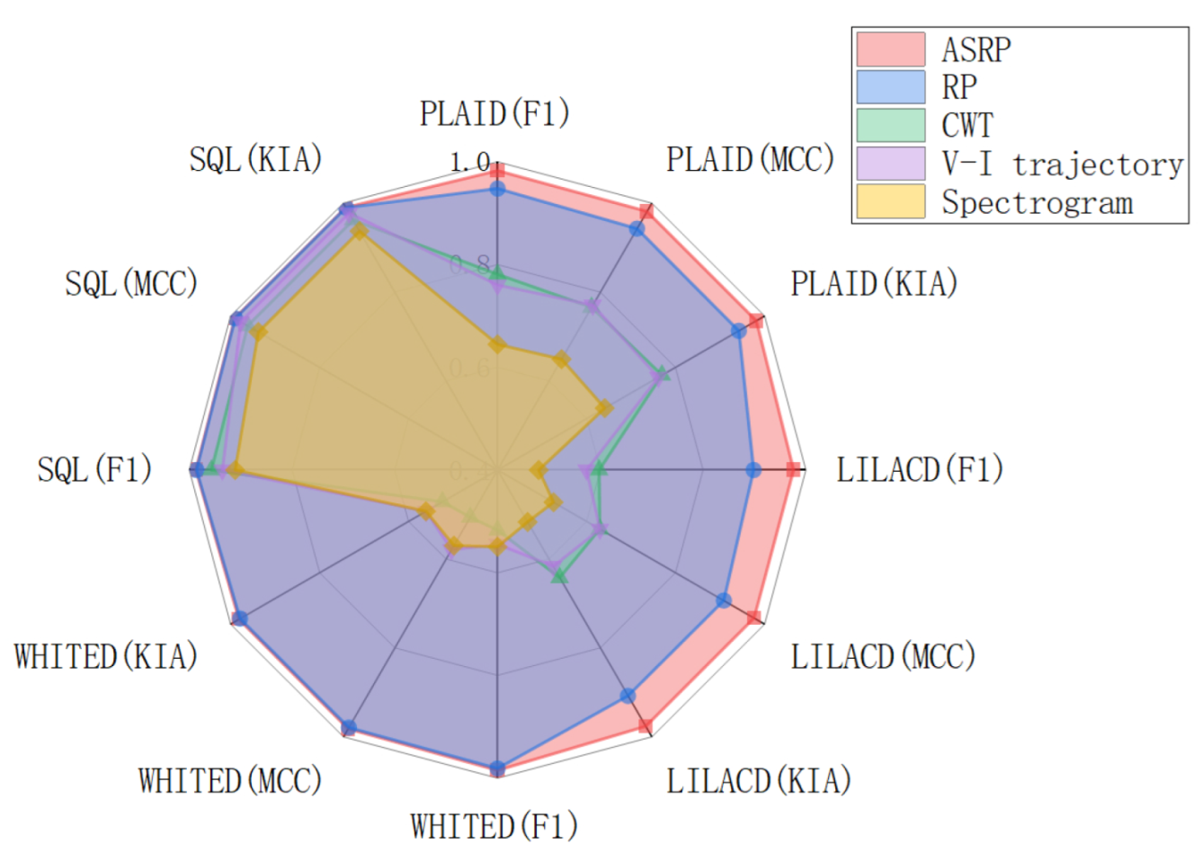
| Dataset | Method | F1 | MCC | KIA |
|---|---|---|---|---|
| PLAID | ASRP | 0.9826 | 0.9814 | 0.9815 |
| RP | 0.9479 | 0.9421 | 0.9427 | |
| CWT | 0.7811 | 0.7658 | 0.7695 | |
| V-I trajectory | 0.7603 | 0.7613 | 0.7708 | |
| spectrogram | 0.6444 | 0.6408 | 0.6490 | |
| LILACD | ASRP | 0.9760 | 0.9763 | 0.9764 |
| RP | 0.8981 | 0.9077 | 0.9082 | |
| CWT | 0.5978 | 0.6299 | 0.6421 | |
| V-I trajectory | 0.5731 | 0.6166 | 0.6302 | |
| spectrogram | 0.4798 | 0.5169 | 0.5256 | |
| WHITED | ASRP | 0.9846 | 0.9815 | 0.9817 |
| RP | 0.9813 | 0.9788 | 0.9791 | |
| CWT | 0.5171 | 0.5061 | 0.5237 | |
| V-I trajectory | 0.5445 | 0.5605 | 0.5790 | |
| spectrogram | 0.5497 | 0.5609 | 0.5700 | |
| HASED | ASRP | 0.9870 | 0.9904 | 0.9904 |
| RP | 0.9858 | 0.9897 | 0.9895 | |
| CWT | 0.9567 | 0.9616 | 0.9620 | |
| V-I trajectory | 0.9356 | 0.9775 | 0.9776 | |
| spectrogram | 0.9108 | 0.9368 | 0.9374 |
Publisher’s Note: MDPI stays neutral with regard to jurisdictional claims in published maps and institutional affiliations. |
© 2022 by the authors. Licensee MDPI, Basel, Switzerland. This article is an open access article distributed under the terms and conditions of the Creative Commons Attribution (CC BY) license (https://creativecommons.org/licenses/by/4.0/).
Share and Cite
Shi, Y.; Zhao, X.; Zhang, F.; Kong, Y. Non-Intrusive Load Monitoring Based on Swin-Transformer with Adaptive Scaling Recurrence Plot. Energies 2022, 15, 7800. https://doi.org/10.3390/en15207800
Shi Y, Zhao X, Zhang F, Kong Y. Non-Intrusive Load Monitoring Based on Swin-Transformer with Adaptive Scaling Recurrence Plot. Energies. 2022; 15(20):7800. https://doi.org/10.3390/en15207800
Chicago/Turabian StyleShi, Yongtao, Xiaodong Zhao, Fan Zhang, and Yaguang Kong. 2022. "Non-Intrusive Load Monitoring Based on Swin-Transformer with Adaptive Scaling Recurrence Plot" Energies 15, no. 20: 7800. https://doi.org/10.3390/en15207800
APA StyleShi, Y., Zhao, X., Zhang, F., & Kong, Y. (2022). Non-Intrusive Load Monitoring Based on Swin-Transformer with Adaptive Scaling Recurrence Plot. Energies, 15(20), 7800. https://doi.org/10.3390/en15207800