Optimization Process Applied in the Thermal and Luminous Design of High Power LED Luminaires

Abstract

This work proposes the design of an optimization method for high-power LED luminaires with the introduction of new evaluation metrics. A luminaire geometry computational method is deployed to conduct thermal and optical analysis. This current effort novels by designing a tool that enables the analysis of uniformity for individual luminaire over the target plane in accordance with international regulatory standards. Additionally, adequate thermal management is conducted to guarantee nominal operation standard values determined by LED vendors. The results of this optimization method present luminaire models with different geometries that allow the stabilization of the temperature within the safety and uniform illuminance distribution thresholds. The resulting solution proposes the design of a $2\times 2$ HP-LED rectangular luminaire. During simulations, the temperature of the LED reaches a maximum value of $73.9$ ${}^{\circ }$C in a steady state with a uniform index of $0.228$ for its individual luminaire. The overall uniform index identified for two separate and adjacent luminaire points in a pedestrian walk is $0.5413$ with a minimal illuminance of $36.95$ lx, maximum illuminance of $93.65$ lx and average illuminance of $68.27$ lx. Overall, we conclude that the currently adopted metric, which takes into consideration only the ratio between the minimum and the average illuminance, is not efficient and it cannot distinguish different luminaire geometry standards according to their uniform illuminance distribution. The metric proposed and designed in this work is capable of evaluating illuminance and thermal threshold criteria, as well as classifying different sorts of luminaries.

1. Introduction

Artificial lighting represents an area of research that has a high consumption of electricity, as it is considered an essential application for quality of life [1,2,3,4,5,6,7]. In the absence of natural light, it makes it possible to carry out commercial and leisure activities, among many others, in addition to promoting a feeling of security. This dependence on searches for energy efficiency in lighting sources is a challenge for researchers around the world [2,4,5,8]. Solid state light sources (SSL) have made progress in recent years, with light-emitting diodes (LEDs) being their biggest representative. These have progressed in terms of improving lamp efficiency and color quality to compete and even surpass traditional technologies in various applications [3].

LED’s compact size allows optical designs to be more flexible. Additionally, LEDs incorporate other advantages when compared to traditional lighting sources, such as: (i) long lifespan, (ii) high brightness, (iii) low power consumption, (iv) fast response, (v) compact size, (vi) high reliability [3,9,10] and (vi) mechanical shock and vibration resistance [11]. However, there are still some difficulties in using luminaires with high-power LED (HP-LED). In addition to the high financial cost compared to other lighting technologies, there are other critical problems that constitute barriers to be overcome by this technology, such as (i) thermal dissipation that can degrade luminous efficiency, (ii) optical performance, and (iii) format of the region to be illuminated [12]. These difficulties are challenges in interior and exterior lighting design when using HP-LED [13].

To improve the design of outdoor lighting, Japanese researchers develop a luminaire with 700 white LEDs for street lighting. The white glow is obtained through a source that emits rays close to ultraviolet in a medium with multiphosphate materials. The project includes a prototype of a self-sustained light pole formed by the luminaire, solar energy plates, and batteries [1]. White LED has superior characteristics of luminous efficiency (40 lm/W) and a color rendering index of about 0.93.

Wang et al. [14] proposes an 80 W streetlamp composed of a combination of 5 W and 3 W LEDs, in which optical analysis is carried out through experimental tests and numerical simulation. A test region of 20 m × 10 m is defined at a height of 8 m from the ground. Numerical simulation results demonstrate that the average illumination is around $8.25$ lx and the uniformity (uniformity is defined as the ratio of the minimum illuminance to the average illuminance in a specific plane) total is $0.364$. Luminaire achieved satisfactory performance, despite the multiple shadows, which need to be removed through optimization techniques.

Bender et al. [15] develop a LED luminaire project for public lighting using mathematical modeling that calculates the total luminous flux considering losses such as light depreciation, dirt on the luminaire, efficiency, and utilization factor. A prototype with 30 LED is built and used in practical experiments seeking to validate the simulation methodology. Spatial diagrams obtained are in accordance with the standards of the Brazilian standard (NBR) 5101:2012 of the Brazilian Association of Technical Standards (ABNT). The method presents itself as a tool to calculate the amount of luminous flux needed for LED luminaires, optimizing the uniformity of lighting and luminance with the use of lenses, to guarantee current standards for public lighting.

Liu et al. [16] seek to standardize the lighting of areas through the mixture of colored LEDs. The proposal for a colored LED luminaire aims to standardize the rectangular lighting pattern by optimizing the arrangement of the 36 LED matrix of the luminaire and the shape of the individual lenses of each LED unit. In the lens optimization process, the Downhill simplex algorithm is adopted and the difficulties are the selection of optimization variables and the reconstruction of the model. An array of $3\times 3$ LED modules, in which each module consists of four lenses optimized for four color LEDs, gives the desired result with color uniformity. The color mixing method appears to be feasible and practical, requiring further studies. As technology advances, new LEDs of higher power and efficiency emerge. However, there is still the problem of heating the LEDs which reduces the luminous efficiency. There are several efforts that present analysis of thermal dissipation of HP-LED lamps and luminaires [17,18]. However, several studies are not concerned with thermal and photometrical analysis concomitantly [19].

Chi et al. [19] present a detailed thermal analysis of a luminaire consisting of three 1 W LEDs. The photometrical analysis is restricted to experimental tests in order to find the relationship between junction temperature and luminous flux. Based on the results of these experiments and using the finite element method, the authors propose a model of the lighting module, simulating, analyzing, and validating the thermal analysis. Simulation results are obtained with values close to the experimental data, with a 6.3% deviation. Once the model is validated, predictions are made in which it is possible to obtain a reduced junction temperature and a more efficient light output, when the number of fins and the opening radius of the lamp are increased.

Bender et al. [20] present methodology for optimized design of LED lighting systems. The purpose of optimization is to provide designers with an ideal operating point, considering the characteristics of the thermal, electrical, and optical systems. The authors consider the output current of the driver circuit, the size of the heat sink, and the temperature of the LED junction in the system design. Mathematical analysis is presented, and the results of the thermal simulations and experimental tests validate the proposed methodology. Bender et al. [21] propose a solution for a streetlight consisting of 30 LEDs and a forced air convection system in a closed cooling cycle. The methodology presented by the authors obtains satisfactory results and is indicated as a tool for the evaluation of thermal projects in LED luminaires.

Some studies present an evaluation of LED reliability and the influence of temperature on other parameters, such as Mean Time To Repair (MTTR) and Mean Time Between Failures (MTBF) [22,23]. Shailesh et al. [24] carry out a review of methods for evaluating the reliability of LED luminaires using thermal measurements. The aim of the work is to develop a mathematical thermal model of the LED luminaire and validate it, reducing the need for experimental analysis. The study models the optical, electrical, and thermal properties of the LED luminaire to assess its performance reliability under various environmental and operational conditions. Thermal management of the LED module is one of the key points of the project, Huaiyu et al. [25] present a review of passive thermal solutions used in LED modules, in which the authors present several thermal interface materials that have a high potential for improving the thermal performance of the module. For commercial LEDs with power consumption below 50 W, the authors report that passive heatsinks are theoretically sufficient for thermal management, with heatpipe technology being the future, due to the advantages of thermal performance, but still at a high monetary cost.

Jakovenko et al. [26] present thermal simulation of an 8 W commercial LED light bulb using finite element methods. Simulated thermal distribution is validated and a parametric study of materials is carried out to discover the problems that occurred in the heat transfer from the HP-LED to the environment. The intentions are to predict the thermal management by simulation and obtain the effect of the lamp shaping and of materials used, to design more efficient LED lamps. The results obtained agree with the desired objectives, however, improvements in the simulation model and parameters result in a better prediction of the measured temperature values. In luminaire projects, there is a tendency to use HP-LED grouping to obtain sufficient luminous flux for lighting a certain area [8,27]. The success of luminaire designs from HP-LED arrays is heavily dependent on thermal management performance, as high operating temperature directly affects light output, quality, reliability, and lifespan.

Luo et al. [28] analyze the thermal distribution in an 80 W HP-LED luminaire, in which the authors use sixteen thermocouples to measure the temperature at different positions of the luminaire and then use numerical simulation to analyze the temperature distribution on the luminaire’s surface. A numerical model is validated and the results of the thermal resistance analysis show that at a temperature of ≈45 ${}^{\circ }$C on the surface of the luminaire, the maximum temperature of the LED crystal junction is equal to the critical temperature of 120 ${}^{\circ }$C, which leads to low reliability, shorter lifespan and lower optical efficiency of the luminaire. Christensen e Graham [29] propose a thermal resistance network model combined with a 3D finite element submodel for the LED structure, in an attempt to predict the temperatures in the LED clusters and the unit chip. Active and passive cooling methods are tested and the impact of LED matrix density and LED power density is evaluated. The conducted analysis suggests the need to use active cooling in luminaires formed by compact HP-LED arrays for operation within the maximum temperature limit of 130 ${}^{\circ }$C.

Luo et al. [30] propose modeling and optimization of the 112 W HP-LED street light heatsink geometry. Experimental results demonstrate that the maximum heatsink temperature remains stable at ≈45 ${}^{\circ }$C when the luminaire is at a temperature of 25 ${}^{\circ }$C. Comparing the results obtained in the modeling with the results obtained in the experiment, it is observed that the proposed methodology is viable and functional for the case of the horizontal heat sink of HP-LED lamps. Scheepers e Visser [31] implements the detailed and computationally efficient HP-LED model. The authors use a gradient-based optimization algorithm, known as the DYNAMIC-Q method, which is applied to maximize the luminous flux output by optimizing power dissipation and thermal resistance. In addition to the geometric parameters of the heat sink, such as the amount, thickness, and height of the fins, the electrical operating current is also evaluated. Luminous flux of ≈42% greater than the initial luminous flux is achieved.

Tang et al. [32] propose 30 W HP-LED luminaire heatsink geometry optimization. The model is simulated and validated through thermocouples and infrared images, showing an error $\le 5.6\%$. Taguchi optimization method is implemented to find optimal values for the amount, width, and thickness of the heatsink fins. Optimized geometry provides weight reduction of ≈33.4% and LED junction temperature reduction from $80.22$ ${}^{\circ }$C to $51.96$ ${}^{\circ }$C. Jeong et al. [33] develop a method of cooling the heat sink of HP-LED luminaires using fin optimization. The model proposed by the authors introduces openings in the base of the heatsink and the fins, improving air circulation. Response Surface Methodology (RSM) is used to optimize the heatsink geometry and the performance of the proposed model is compared with that of conventional heatsinks. The total thermal resistance of the model is reduced by 30.5% and the luminous efficiency increased by 23.7%. In addition, the financial costs of production are reduced, as the total volume of the model is 30.4% smaller.

Several efforts have carried out thermal studies of LED luminaires, each with its own peculiarity [19,21,25,26,28,29]. There are several methods for optimizing heatsink geometry parameters to reduce the LED junction temperature [20,30,31,32,33]. Other studies focus on the photometrical analysis of the HP-LED luminaire, addressing the luminous uniformity on the target plane [1,13,14,15]. The application of the optimization process in lenses and coupled optical systems is presented in the studies of [16,34,35].

There are several studies indicating prototypes of LED luminaires, in which some use analytical methodology (deterministic methods), others with numerical methodology (based on FEM), and others incipient using heuristic methods. Most methodologies use confined environments (internal environments) and methodologies that work with external environments are also incipient [36]. There is a need to develop methods that include the new technologies of HP-LED lamps and luminaires applied to the lighting of large areas and outdoor areas. The proper design of an efficient lighting source represents high financial and environmental savings, as the best way to illuminate the intended region is the most economical and self-sustainable. The study that covers simulation by numerical methods, optimization by heuristic and deterministic methods together, and that is carried out for the system in an external environment, justifies this work.

The originality of the present study is the creation of a methodology for optimizing luminaire parameters, focusing on both the luminous and thermal aspects. The novelty of this work lies in the study of the sensitivity analysis of parameters to be applied in the optimization process, seeking to substantiate the importance of the selected parameters in the search for optimal/optimized results. Hence, the application of this new approach is relevant, which can generate cost savings for private and public entities with better specifications of lighting products, producing reasonableness. With the proper specification, HP-LED lighting products tend to have a longer lifespan with proper temperature management and an evenly lit environment prevents both excess and shortage of bright spots. The new technique presented has applicability in lighting areas with greater application in pedestrian and vehicle traffic lighting.

This work aims to develop an optimization methodology for designing HP-LED luminaires that present uniformity in the illuminated area according to references established by standards and adequate thermal management, ensuring luminous flux and valuable life in the nominal standards. The specific objectives are: (i) design a computational model of LED luminaire geometry, (ii) perform thermal and optical analysis through a simulator, and (iii) optimize luminaire geometry and LED matrix arrangement to standardize the lighting on the target plane, keeping the temperature of the LEDs below the maximum allowed values.

This work is structured as follows: in Section 2 concepts related to theoretical foundations, the basis for understanding, the methodology, and results, Section 3 describes the work methodology, with the procedures, materials, and methods used. In Section 4 the results obtained from the application of the proposed methodology are displayed and the conclusions are exposed in Section 5.

2. Theoretical Background

This section presents a brief description of electric lighting technologies, the financial costs involved in artificial lighting, and the search for energy efficiency with a focus on lighting. A brief description of the used simulators is exposed, and finally, the theory that involves the parameter sensitivity analysis is presented.

2.1. Artificial Lighting Environments

In terms of environments, there are two types of artificial lighting: (i) for indoor areas and (ii) for outdoor areas. Artificial lighting for indoor areas is applied to homes, businesses, and industries. In this type of application, operating conditions are independent of weather and environmental conditions such as wind, rain, fog, and traffic situations [5,9,37]. As there is a wide range of applications for this case, consequently there are different requirements and objectives to be met. There are international standards that must be followed in indoor lighting projects [9].

Artificial lighting of external areas (public lighting), such as streets, roads, bridges, tunnels, parking lots, monuments, and building facades, among many others, can be classified as road, urban, and monumental. In general, it provides the inhabitants of urbanized areas with the freedom to fully enjoy public space at night, in addition to preventing/reducing crime. Adequate public lighting guides pathways and beautifies urban areas [5,37]. As with artificial lighting for indoor areas, there are international standards that regulate the specifications required for each application of artificial outdoor lighting.

2.2. Light-Emitting Diodes Technologies

The LEDs can be classified according to the power consumed and, consequently, the brightness emitted. Low power LEDs are characterized by low supply current, close to 20 mA and low power, approximately 44 mW. Since the 1970s, they have been used in the most varied applications, such as cell phone backlights, pushbuttons, flashlights, display screens, and road signage, among others. They can be found in the colors: red, orange, green, yellow, and blue. Essentially, these types of LEDs are used as indicators and not as a light source [38,39].

Medium power and high brightness LEDs have power from 1 W to 3 W and supply current of 30 mA, 75 mA or 150 mA [39]. HP-LEDs and ultra-high brightness LEDs are characterized by powers above 3 W. Higher powers imply higher luminous flux and supply current in the range of 350 mA to 6 A [39,40]. Both devices have been replacing traditional light sources in several applications.

In LED lighting design, the use of single-chip limits the luminaire, making its use in several applications impossible. Multichip LEDs have four to six chips in the same package, increasing the luminous flux of the device. However, two problems challenge the luminaire design: thermal dissipation and the proper direction of the luminous flux. LED multi-chips face more difficulties than other solutions on both issues. Die concentration in a small area makes thermal management a critical factor, as higher temperatures mean lower luminous efficiency. In addition, another disadvantage is the non-uniform nature of the light source. The gaps between the arrays are black areas that when projected by the optics lead to non-uniformity of the light output beam over the target plane [41].

A second option is the use of COB LEDs, multiple LED chips packaged together as one lighting unit. Due to their compact size with high luminous flux, they have several advantages for the design of luminaires. However, the COB LED chip junction temperature is still a disadvantage in critically high hot spots [42]. Another alternative is the use of single-chip LED arrays, generally SMD, distributed in the luminaire to increase the emission of the final luminous flux [27,43]. This technique allows generating multidirectional luminous flux and facilitates thermal management.

2.3. Financial Costs of Artificial Lighting

According to the annual energy report prepared by the Energy Information Agency of the United States Department of Energy, it is estimated that the demand for electricity in the US is projected to grow by $0.8\%$ per year on average, from 2013 to 2040 [44]. This represents $21.6\%$ over the estimated 27 years. In the same period, total electricity generation capacity, including capacity in end-use sectors (end-use sectors comprises the building sector—residential and commercial-, industrial and transport), is projected to grow by ≈18.4%, from 1.065 GW in 2013 to 1.261 GW in 2040 [44].

The need to manage the use of electrical energy becomes a reality. The search for energy efficiency in lighting, in addition to bringing benefits such as the reduction of expenses with electricity consumption, helps to preserve the environment [37]. However, lighting that meets energy efficiency requirements cannot be of poor quality (shade or glare, reduces the amount of light needed to have lighting of the desired quality, depending on the environment, the types of surfaces present and the type of activity to be carried out in this environment, according to references that specify standard values for each situation). Low-quality lighting affects aspects such as safety, health, performance, and comfort, among others [45].

The current model of the lighting market is composed of four sectors: (i) residential, (ii) commercial, (iii) industrial, and (iv) external which is subdivided into eight sub-markets [5,46]. In 2014, 33 billion light bulbs were operating in the world, consuming more than 2.650 TWh of energy per year [8]. Approximately 20% of total electricity consumption is spent on artificial lighting and this consumption pattern is repeated in all countries [1,2,3,8]. Figure 1, adapted from Almeida et al. [8], illustrates the distribution of world electricity consumption for each sector of the lighting market model.

The outdoor sector of the market model is primarily exemplified by public lighting. This percentage represents an important and costly responsibility for the directors, consuming $\frac{1}{3}$ of the cities’ total energy bill [47,48,49].

2.4. Light System and Heat Transfer System Simulators

It is possible to use computational routines to simulate the dynamics of processes through coherent modeling that describes the physical interactions. Simulators reproduce results similar to those found in real processes through extensive processing of mathematical and physical calculations, reducing the need for practical tests and consequently reducing the time to determine how the system responds to systematic changes in its parameters. In addition to time, simulation reduces financial costs and prevents irreversible damage to devices and equipment [50].

There are several lighting system simulators based on techniques such as ray-tracing, ray-launching, and finite element methods (FEM). The ray-tracing simulator has a lower computational cost than the FEM and allows you to configure different lighting patterns of the emitting source and adjust various optical parameters [51,52]. Input variables are the light source parameters (angular intensity and power), primary and secondary optical accessory geometry parameters (spatial position, lens, and reflector dimensions), detector parameters (target plane area and distance to the source ), and simulation configuration parameters (number of rays).

Several simulators are based on numerical simulation techniques to solve problems involving heat transfer models. Three major strands are finite differences, finite elements, and boundary elements. There is no superior method in all cases, as each method has its advantages and disadvantages [53]. Input variables of the simulator are the parameters of the heat source (size, power, and transmission coefficients), parameters of the geometry of the heat sink base (length, width, height, and the number of fins), parameters of the mesh elements and parameters of the physics involved in the process.

2.5. Parameter Sensitivity Analysis

In possession of the model or the real system, it is possible to study the effect of a given input on a given output, seeking to quantify the relative contribution of each input variable to the output. Such analysis makes it possible to eliminate certain parameters that have insignificance in the response, to define input variables that contribute to the variability of the output, to understand the consequences arising from the change of a certain input parameter, among others [54,55].

Input parameters refer to variables that can be manipulated, while output parameters refer to variables affected by this manipulation. The manipulations of input parameters can be classified according to the approach adopted in relation to the search space, which can be local or global. In the local analysis, the outputs obtained are evaluated by varying a given input parameter at a time, keeping the other parameters fixed at the base value. In a global analysis, outputs are obtained globally by averaging over the range of all input parameters [54,56].

To measure the contribution of each input variable to the output variability, visual, analytical, and statistical methods can be used depending on the purpose [54,56]. In the local approach, known as one-at-a-time, the base-value solution consists of parameter values that produce an optimal/optimized solution or expert-suggested values that are expected to obtain an optimal/optimized solution. From the base value, the parameter can be varied in the range [$-100\%,+100\%$] or up to the limit of its range of viable values [55]. The graphical analysis of the response curves as a function of the input parameters using the one-at-a-time approach produces a diagram with a peculiar format, called spider graph [54,57,58].

These methods result in sensitivity measurements providing conditions that support decision-making on issues related to model simplification, optimized solution robustness, and error checking, among others [55]. In this regard, Saraiva et al. [59] proposes five methods for determining the sensitivity indices of each input parameter through the analysis of the spider graph obtained by the one-at-a-time approach.

2.6. Applied Optimization Process

The optimization process is the mathematical study that aims to solve a problem through the search for parameters that result in an optimal or optimized solution. Mathematically, we seek to maximize or minimize the function $f\left(x\right)$ through the systematic choice of parameters within a set of viable solutions $\Omega$, resulting in the end of the optimized solution $f\left(x^{*}\right)$. The choice of optimization method to be applied depends on the nature of the problem and should not influence the result. The problem variables become parameters that make up the solution and their values are sequentially modified to reach the optimized solution. The way in which each algorithm proceeds in calculating the direction of adjustment of these variables and the dimension of this step at each iteration makes up the strategy. This strategy used to go from one iteration to another is what distinguishes one algorithm from another [50].

The quasi-Newton method belongs to the class of methods that use derivatives. It is an iterative technique that seeks to find the stationary point where the gradient is zero. For this, it uses the information from the gradient of the evaluation function in each iteration, measuring its changes. It is the intermediate method between the simplicity of the gradient method and the speed of Newton’s method [60]. Figure 2 illustrates the flowchart of the Quasi-Newton method.

Nelder-Mead method, or flexible polyhedra, is the direct search technique that does not use numerical or analytical gradients. His algorithm is applied to unconstrained and nonlinear optimization problems, whose derivatives are not known or the evaluation function is not differentiable. It starts with a set of points that form the simplex. At each iteration, the values of the evaluation function at the vertex points of the simplex determine the worst point. The algorithm replaces the worst point, introducing a new vertex so that it results in a new simplex. Candidate replacement points are obtained by transforming the worst vertex through a series of operations on the centroid of the current simplex: reflection, expansion, contractions inside and outside the polyhedron [61]. Figure 3 illustrates the flowchart of the Nelder-Mead method.

Biogeography-based optimization (BBO) belongs to the evolutionary algorithm class and is motivated by the theory of species migration between habitats [62,63]. BBO includes migration-based prospecting and exploration strategies. Through mathematical models of biogeography, it is possible to describe: (i) the evolution of new species (speciation), (ii) the migration of species between islands, and (iii) the extinction of species [64]. BBO algorithm has parameters that must be adjusted to better meet the specificity of each problem to be solved. The initial population is of constant size, generated randomly, and replaced every generation. The immigration probability values define whether a given independent variable of the candidate solution is substituted. The mutation operator must define a probabilistic function that can modify the characteristics of the solution. The desired solution corresponds to the biological habitat suitable for life (high habitat suitability index—HSI). Figure 4 illustrates the flowchart of the BBO method.

Genetic algorithm (GA) is an evolutionary optimization technique based on a metaphor of the biological process of natural and genetic evolution [65,66]. It is a robust search technique that scans the solution space and finds solutions close to the optimal solution. Its robust nature refers to the ability to perform efficiently on a wide range of problems, not requiring the problem to have particular requirements to be solved. [66]. In classical GA, the population is a matrix of constant size $p\times g$ and is initially generated randomly, where p is the number of individuals and g is the number of genes in each individual. Each gene receives the value of a variable of the problem and each individual of the population is a possible solution to the proposed problem and its quality measure is performed through the evaluation function [67]. After being evaluated, the population is submitted to genetic manipulators, elitism, and selection, and then to crossover and mutation operators. Figure 5 illustrates the flowchart of the GA method.

2.7. Measurement Standards

Standards CIE 115:2010—Lighting of Roads for Motor and Pedestrian Traffic, CIE 136:2000—Guide to the lighting of urban areas, IESNA/ANSI:2014 RP-8—Roadway Lighting and BS 5489-9:2013 provide quantitative recommendations for external lighting, which can be vehicular and pedestrian traffic highways and urban streets. In general, the height of assembly of lighting points that involves vehicular traffic is defined from 7 m to 12 m and the uniformity between 0.35 to 0.40, according to parameters that involve variables such as volume and speed traffic, road complexity, and others. For lighting in places that involve pedestrian circulation, such as squares and parking lots, the standard does not define the exact height of the lighting point, stipulating that the average illuminance must be at least 3 lx and uniformity of 0.20. However, it appears that the standard used in this context is from 3 m to 5 m.

ISO/CIE 8995-1:2002—Lighting of workplaces—Indoor, recommends standards for indoor lighting, specifically in work environments. In this case, the height of the lighting point is close to the height of the room, which varies between 2.5 m to 2.8 m for properties with simple ceilings and the illuminance varies according to the activity performed, being generally greater than 100 lx and uniformity greater than or equal to 0.60.

Regarding the illuminance measurement methodology and subsequent uniformity calculation, the standards CIE 140:2000—Road Lighting Calculations and EN 13201:2016—Road Lighting, establish a mesh of points on the target plane. For work environments, it is recommended that the illuminance from 9 to 36 points on a given target plane should be measured. For public lighting for vehicular traffic, a grid is also established consisting of fifteen measuring points per roadway arranged between the two axes of the luminaires. For pedestrian sidewalk lighting, the mesh of points is dependent on the width of the sidewalk.

3. Methodology

This section proposes the development of an optimization methodology for the design of a high-power LED luminaire that meets luminous and thermal requirements. The luminaire must have lighting uniformity in the target plane according to standards established by international standards. Thus, the thermal management of HP-LEDs is necessary to guarantee luminous flux and useful life according to nominal standard values. For this purpose, techniques and tools used in the analyzes carried out in rectangular luminaires with matrix arrangement of multiple HP-LEDs are presented. Optimization methods are specified and the multi-objective evaluation function is defined.

3.1. Analysis, Simulation and Practical Test of the Thermal-Luminous Effects in a $m\times n$ Luminaire

The analyzes are carried out for rectangular luminaires composed of a matrix arrangement of $m\times n$ HP-LED fixed on an aluminum dissipative base located on the face opposite the luminous flux output. The variables m and n assume any integer values $\ge 1$ and do not necessarily have to be equal. For this case, computational and experimental simulation analyses are conducted. The thermal analysis of the luminaire is proposed to verify if the temperature conditions are being met to provide the nominal lifespan of the HP-LED. In the thermal modeling of the luminaire, specific software is used that simulates the heat transfer with the finite element method (FEM). The methodology of thermal analysis and validation of this luminaire is described in Barbosa et al. [46], in which the authors perform the simulation considering the static model in three-dimensional geometry. The simulated three-dimensional model of the HP-LED is illustrated in Figure 6.

The photometrical analysis is performed using optical simulation software, with the aim of verifying whether the lighting uniformity conditions meet the standards of international standards. The methodology of light analysis is described in Barbosa et al. [68], in which the authors use an optical simulator based on the ray-tracing technique. Modeling is performed in non-sequential mode, in which the order of intersection of the rays on the surface is not known. Therefore, when colliding with the surface, the ray may reflect, refract, diffract, scatter and/or split into small rays. Since image formation is not necessary, the rays do not act in a certain way and there is no image caveat (points do not need to map points), so several rays must be traced to analyze the performance of the LED model.

3.2. Luminaire Optimization Process

In this work, the purpose of the optimization is to find the luminaire parameters that provide satisfactory results in both thermal and luminous analyses. The optimized luminaire must satisfy the thermal dissipation requirement in which the LED chip temperature is kept below the junction temperature (defined in the datasheet) and must provide homogeneous illumination in the target plane. Some luminaire parameters are directly selected based on the influence of heat dissipation.

Table 1. Geometric parameters referring to heat dissipation.

Parameter	Description
m	number of LEDs arranged along the length of the heatsink base
n	number of LEDs arranged in the width of the heatsink base
$Wh$	heatsink length [mm]
$Lh$	heatsink width [mm]
$Hh$	heatsink height
$Nf$	number of fins present in the heatsink base
$Hf$	heatsink fin height
$Wf$	heatsink fin length
$Tilt$	inclination degree of LED rows in matrix arrangement [${}^{\circ }$]

shows some parameters that change the geometry and arrangement of the luminaire and they are illustrated in Figure 7. After parameter sensitivity analysis, six parameters were selected among those presented, such as: m, n, $Wh$, $Lh$, $Nf$, $Tilt$. In the optimization process, there are parameters related to the systems that are fixed and must be defined in advance, in which

Table 2. Simulation parameters.

Parameter	Description
$H_P$	luminaire height above the target plane [mm].
$X_P$	target plane width [mm].
$Y_P$	target plane length [mm].

has some of these parameters.

When the purpose of optimization is to minimize the temperature of the LED, the immediate solution is to produce a luminaire with a smaller number of LEDs arranged in the largest possible area of the heatsink base. However, the number of LEDs and their arrangement in the luminaire directly affect the distribution of the luminous flux in the target plane. Figure 8a illustrates a hypothetical example of illuminance on the target plane produced by an HP-LED luminaire in a matrix arrangement, showing the lighting points corresponding to the LED sources. When drawing a horizontal line in the center of the Figure 8a (cut line), on the x axis, illuminance locations with different values are observed. From this abstraction, it is possible to build the mapping of illuminance values, as illustrated in Figure 8b.

As an alternative to the calculation proposed by the European standard to measure non-uniform HP-LED radiation patterns, Barbosa [50] produces a numerical evaluation model that measures the illuminance values along the cut-off line, having as one of the metric parameters the desired value. Figure 9, adapted from Barbosa [50], illustrates the example of the measured illuminance distribution curve $S_q$ as a function of the position on the coordinate axis x in the target plane, together with the desired illuminance curve $D_q$.

The difference between the measured illuminance curve and the desired illuminance curve is the proper metric to quantify the quality of uniformity over the target plane. The metric developed in Barbosa [50] to measure the quality of uniformity over the target plane is given by:

$$f_{Lp}\left(x\right)=\sum _{q=1}^k∥\frac{[(D_q-S_q)+(D_{q+1}-S_{q+1})]·{\Delta }_q}{2}∥$$

(1)

where ${\Delta }_q$ is the difference between the points on the coordinate axis x between q and $q+1$, where $q\in \{1,2,3,\dots ,k\}$ and k is the number of discretized points on each illuminance curve. In a hypothetical simulation with a four-LED luminaire and a target plane of $X_P\times Y_P$, the illuminance values are extracted along the coordinate axis x at the center of the target plane (at $y=0$). Therefore, the output results profile is defined by setting the value of y to $zero$ which would return all illuminance values for each coordinate x.

The metric created to measure the quality of the candidate solution calculates the area between the desired and simulated illuminance along the x coordinate axis at $y=0$. As there is partial symmetry between the longitudinal axis x and the longitudinal axis y of the luminaire, it is expected to find the same sensitivity index for the parameters m and n, as well as for $Wh$ and $Lh$. However, the results presented in trials do not confirm this expectation. The difference is due to the way the valuation function is calculated, as the valuation is performed only on the coordinate axis $y=0$ (horizontal valuation). As a consequence, the luminaire with a hypothetical LED arrangement of 2 × 4 will have a different evaluation function than the luminaire with a hypothetical LED arrangement of 4 × 2, since there is no evaluation of the result on the axis of coordinates y (in $x=0$).

Once this fact has been verified, it is necessary to create an evaluation profile on the y coordinate axis to verify the illuminance behavior also on the vertical axis and to avoid discrepancies in the results for symmetrical solutions. Additionally, new evaluation profiles must be defined parallel to the central axes $x=0$ and $y=0$ to expand the verification of the uniformity of the luminous flux in the target plane and thus, obtain better solutions. In this new proposal, the number of evaluation profiles must be selected on the coordinate axis x and on the coordinate axis y and the position of these profiles along the axis. In case there are three evaluation profiles on each coordinate axis, you can define the evaluation profiles: (i) x in $y=0$, $y=-Y_P/4$, $y=+Y_P/4$ and (ii) y in $x=0$, $x=-X_P/4$ and $x=+X_P/4$. The six evaluation profiles are illustrated in Figure 10.

The use of more longitudinal profiles parallel to the axis $y=0$ corroborates the recommendations of international standards, which specify the inspection procedure for illuminance uniformity. On vehicle traffic lanes, a mesh of measurement points must be generated between two lighting points (poles) in which three longitudinal lines and five transverse lines are defined for each lane. In the case of people traffic (sidewalks), the procedure recommends two longitudinal lines. The final illuminance evaluation function is re-defined as the arithmetic mean of $f_{Lp}$ in (1), applied over n-coordinate axes profiles, given by:

$$f_L\left(x\right)=\frac{1}{n}·\sum _{p=1}^n{f}_{Lp\left(x\right)}^p$$

(2)

where p represents the index of the analyzed profile, n is the number of evaluation profiles, and $f_{Lp\left(x\right)}^p$ is the evaluation function defined by (1) and computed for each profile of each axis. To evaluate the optimization process considering the thermal effects of heat dissipation, a metric that measures the quality of candidate solutions must be obtained. As an improvement to Barbosa’s [46] work, it is proposed to modify the thermal dissipation evaluation function $f_T\left(x\right)$ to assume the shape of the sigmoid function, as illustrated in Figure 11. The new heat dissipation evaluation function $f_T\left(x\right)$ is given by:

$$f_T\left(x\right)=\frac{1}{1+e^{-\lambda (x-\Gamma )}}$$

(3)

In (3), $\lambda$ determines the slope degree of the sigmoid function and $\Gamma$ is the maximum temperature value supported by the LED chip, which must be lower than the junction temperature of the HP-LED. Both expressions (2) and (3) are normalized in the range $\left[01\right]$, in which the final evaluation function $f\left(x\right)$ is the combination of $f_L\left(x\right)$ and $f_T\left(x\right)$ in the proportion given by:

$$f\left(x\right)=\theta ·f_T\left(x\right)+[1-\theta ]·f_L\left(x\right)$$

(4)

where $\theta$ is a number in the range $\left[01\right]$ chosen empirically to give weight between the two components of the final evaluation function $f\left(x\right)$. The optimization process is applied to find the best parameters of the HP-LED luminaire geometry. For each candidate solution, the optimization algorithm runs the thermal simulator evaluating the solutions and then runs the luminous simulator evaluating the results of both combined by (4). This process is repeated iteratively until the optimized solution for the geometry of the HP-LED luminaire is obtained. The optimization problem is given by:

$$\begin{array}{c}minf\left(x\right)\mathrm{subject}\mathrm{to}:\hfill \\ \alpha \le m,n\le \beta \hfill \\ \delta \le Wh,Lh\le \eta \hfill \\ \psi \le Nf\le \gamma \hfill \\ 0\le Tilt\le \zeta \hfill \end{array}$$

(5)

where $x\in \Omega \subset R^p$, $\Omega$ is the search space of independent variables, m and n are the number of LEDs arranged in the length and width of the heatsink base, respectively. The heatsink parameters include $Wh$ and $Lh$, which are the length and width, respectively. The other variables are: $Nf$ is the number of fins on the heatsink base and $Tilt$ is the maximum tilt angle for a given row of LEDs, $\alpha$, $\beta$, $\delta$, $\eta$, $\kappa$, $\phi$, $\varphi$, and $\gamma$ are minimum and maximum values of the parameters to be optimized. In this way, the vector $\overrightarrow{x}$ of the optimization parameters is defined as: $\overrightarrow{x}=[m,n,Wh,Lh,Nf,Tilt]$.

The $Tilt$ parameter is used to define the slope of the LED rows in the matrix array. For example: let the matrix $A_{m\times n}$ represent the matrix arrangement of the HP-LEDs on the heatsink base, in which m represents the i-lines and n the j-columns. The elements of $A_{m\times n}$ are indicated by $a_{ij}$. Thus, the vector $v_1=\left[a_{1j}\right]$ represents all elements of line 1. The parameter $Tilt$ is defined as the inclination angle applied to all elements of $v_1$. This angle is fixed and equal to $\zeta$. Similarly, the vector $v_m=\left[a_{mj}\right]$ represents all elements of the line m where a fixed angle equal to $-\zeta$ is assigned. For the other intermediate row vectors, sub-multiples of $\pm \zeta$ are assigned such as: $\pm \zeta /2,\pm \zeta /3,\cdots$ including $\zeta =0$ used on the central axis when m is odd. Optimization methods are selected to be used in the multi-objective problem and subsequently have their results compared. Two deterministic algorithms and two heuristic algorithms are chosen to be used. In this work, the optimization process is only intended to find the best values of the geometry parameters of the LED luminaire and to compare two deterministic optimization methods with two heuristic optimization methods.

3.3. Presentation, Analysis and Validation

The purpose of this work does not limit the design of a luminaire for internal or external use and can be applied in both cases with the necessary adaptations. The methodology presented in this work aims to optimize the uniformity of the illuminance distribution in the target plane by a luminaire, that is, an isolated lighting point. No standard was found that advocates minimum uniformity in this context. To validate the uniformity of the illuminated region, verifying if it meets the references defined in the standard, the application of pedestrian traffic lighting away from motorized roads is chosen. The illuminance distribution analysis and subsequent uniformity calculation are performed in a target plane interposed by two adjacent sources of illumination and distant from S, with their axes located at the ends of the target plane. The sidewalk width is defined in $W_f$. For measurement, four points are arranged in a reticulated mesh of D in the transverse direction of the road and $d_f$ in the longitudinal direction, as illustrated in Figure 12.

4. Results

In this section, the results obtained from the application of the proposed methodology are presented. First, the main parameters to be used are set out, the results obtained previously in other published works are presented and compared, the optimization process is applied using the new methodology and at the end, the work as a whole is discussed.

4.1. Parameter definition and evaluation function

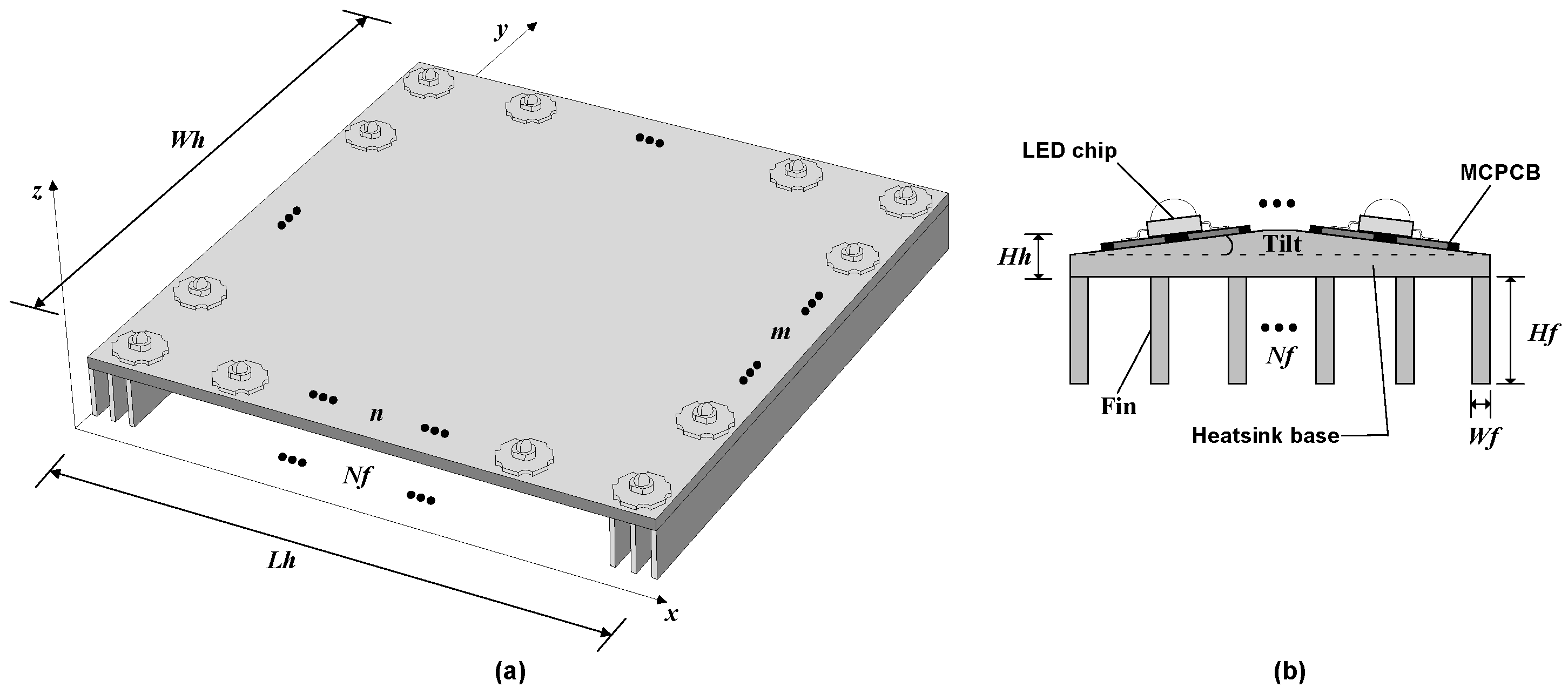
Given the rectangular luminaire model composed of a matrix array of $m\times n$ HP-LED, optimization algorithms are proposed to find the parameters that define the geometry and power of the luminaire. HP-LED power range used in this work is 5 W. Luminaire is fixed at a height of $H_P$ = 2 m above the target plane of dimensions 3 m × 3 m. Parameters manipulated in the optimization process are arranged in Table 1 and restrictions on the search space of each parameter are defined as:

$$\begin{array}{c}minf\left(x\right)\mathrm{subject}\mathrm{as}:\hfill \\ 2\le m,n\le 6\hfill \\ 50\le Wh,Lh\le 300\hfill \\ 2\le Nf\le \gamma \hfill \\ 0\le Tilt\le 10\hfill \end{array}$$

(6)

$$\gamma =\frac{Lh}{16}+0.75$$

(7)

where the value of $\gamma$ in (6) is dependent on $Lh$ on (7). Final evaluation function value in $f\left(x\right)$ (4), was defined for $\theta$, chosen empirically in order to give weight between the two components of the final evaluation function. Thus, the final evaluation function $f\left(x\right)$ is the combination of $f_L\left(x\right)$ and $f_T\left(x\right)$ in the proportion given by:

$$f\left(x\right)=0.4·f_T\left(x\right)+0.6·f_L\left(x\right)$$

(8)

To evaluate the optimization process considering the lighting effects, the expression (2) as a metric to measure the quality of uniformity over the target plane. The new evaluation function is defined as the arithmetic mean of the expression $f_L\left(x\right)$ (1), applied over six coordinate axes profiles: $x=-1000$, $x=0$, $x=1000$, $y=-1000$, $y=0$ and $y=1000$, given by:

$$f_L\left(x\right)=\frac{1}{6}·\sum _{p=1}^6{f}_{L\left(x\right)}^p$$

(9)

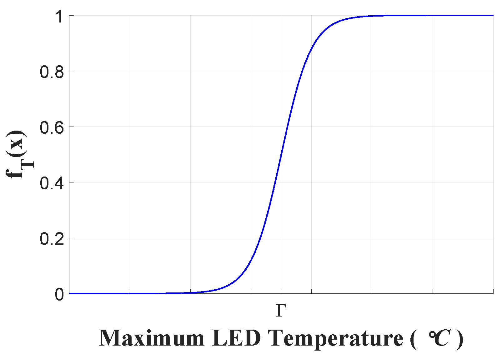
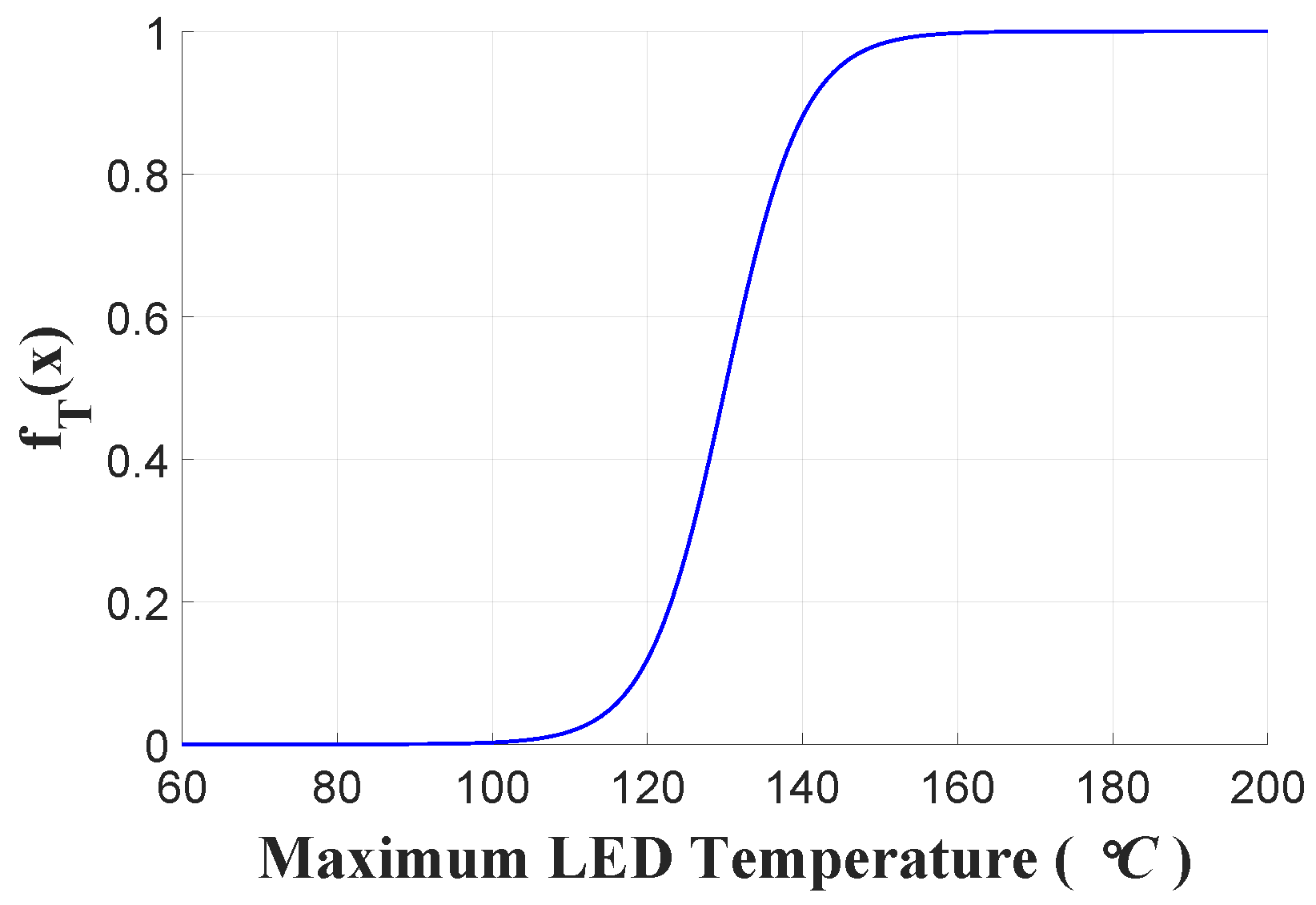
To evaluate the optimization process considering the thermal effects of heat dissipation, the new thermal dissipation evaluation function $f_T\left(x\right)$ is illustrated in Figure 13 and in this way, the expression (3) can be rewritten as:

$$f_T\left(x\right)=\frac{1}{1+e^{-0.1(x-130)}}$$

(10)

Finite element method (FEM) software COMSOL Multiphysics is used to model the physical laws that describe the heat exchange [69]. The thermal analysis is performed using the Heat Transfer Solid module from COMSOL.

Table 3. Material properties.

Material	Thermal Conductivity (W/(m${}^2·$ K))
LED chip (GaN)	130
Slug (Al)	238
Outer plastic	0.18
Plastic lens	0.50
MCPCB	201
Heat sink (Al)	238

shows the thermal conductivities of the materials used in the model. The mesh element number is increased until it reaches grid independence during the thermal simulation. As the geometry of the luminaire is dynamic, i.e., the heat sink dimensions and the number of LEDs vary, the number of elements in the mesh depends on the geometry of the object being simulated. The boundary condition of the simulation model is defined as a room temperature of 27.2 ${}^{\circ }$C, and a heat coefficient value of 5 W/(m${}^2·$K) is used for heat transfer from the heat sink to air (natural convection).

With regard to photometrical analysis, the HP-LED luminaire model is designed in the optical simulation software ZEMAX-EE Optical Design Program includes a stochastic simulation of about one million light rays emitted by each LED and the extraction of the luminous pattern from the target plane [70]. The optimization algorithms aim to find the best geometric parameters for the HP-LED luminaire. For each candidate solution, the optimization algorithm runs the first simulator to perform a thermal simulation and then runs the second simulator to perform a ray tracing analysis. The results of the simulations are combined as in (8).

4.2. Comparison with Previous Results

The methodology proposed in this work implements several improvements when compared to the methodology described in the previous study [46]. One of them is the addition of a new parameter of the luminaire geometry called $Tilt$. This newly proposed parameter allows a certain linear sequence of LED sources parallel to the dimension $Lh$ to tilt at $\pm {\zeta }^{\circ }$. Inserting this parameter produces more uniform lighting results, as the sources (LED) are fixed on a flat base with a different slope in each row of LEDs.

Another improvement implemented is the changes defined in the values of geometric constraints for the parameter $Wh$ and $Lh$ that represent respectively the length and width of the heatsink. The value of $\eta$ is increased from 200 mm to 300 mm so that luminaires with a maximum arrangement of $6\times 6$ LED become thermally viable. Although the lower limiting value $\delta$ of the $Wh$ and $Lh$ parameter is 50 mm in theory, for a $6\times 6$ LED luminaire there is a geometric limitation so that to position yourself in this amount of LED, a minimum value of $Wh$ and $Lh$ of 150 mm is required. Thus, with the change, the real amplitude of the variation range of parameters $Wh$ and $Lh$ becomes $150\le Wh,Lh\le 300$.

A change was implemented in the positioning logic of the heatsink fins, which in the previous work [46], the number of fins on the heatsink base, defined by the parameter $Nf$, has a fixed spacing being positioned from the lateral ends of the heatsink to the central part of it. With the change in logic, the spacing is no longer fixed and becomes dynamic, and symmetrically distributed according to the optimized value of $Lh$. In the optimization process of the previous work [46], a target plane of 4 m × 4 m is used and in the optimization process proposed in this work a target plane of 3 m × 3 m is defined and the value of the font height is increased. The reduction in the dimension of the target plane from 16 m${}^2$ to 9 m${}^2$ was performed to better match the standards used in the distance of lighting points. The area of the target plan is empirically defined, as it seeks to develop a methodology to contemplate the analysis of any application of luminaire (for specific analysis, whether internal or external lighting—of pedestrians or motor vehicles—will exist in each case, specific standard to define maximum height and distance between two illuminated points).

The function of evaluating the illuminance uniformity over the target plane has been changed. Unlike the previous methodology that used only one evaluation profile along the x coordinate axis (in $y=0$), it is proposed to use six evaluation profiles, with three evaluation profiles on the x coordinate axis and three evaluation profiles on the y coordinate axis. Regarding the thermal dissipation analysis, the empirical expression suggested in the initial methodology [46] evaluates the maximum LED temperature values obtained in each simulation according to the distance from the value set as desirable. However, some results indicate the value of the evaluation function $f_T\left(x\right)$ is relatively high even for low values of simulated maximum temperature. Thus, even lower-than-desirable temperature values, which can produce optimal solutions, are penalized in the same way as higher-than-desirable temperature values. To solve this problem, the current proposal presents the modification of the thermal dissipation evaluation function $f_T\left(x\right)$ to assume the form of the sigmoid function.

Finally, in this proposal, another heuristic optimization technique is used to expand the analysis and compare other optimization techniques. A genetic algorithm with real coding (GARC) is used, consisting of the characteristics: (i) tournament selection with $\tau =3$, (ii) simple crossover operator, and (iii) evolutionary mutation operator with 1/5 rule success. In possession of both results, the methodology proposed in this work and previous studies [46], the respective solutions are compared, reassessing/simulating them with all the proposed modifications. The illuminance distribution curves of the three profiles on the x and y coordinate axes are shown in Figure 14, Figure 15, Figure 16 and Figure 17.

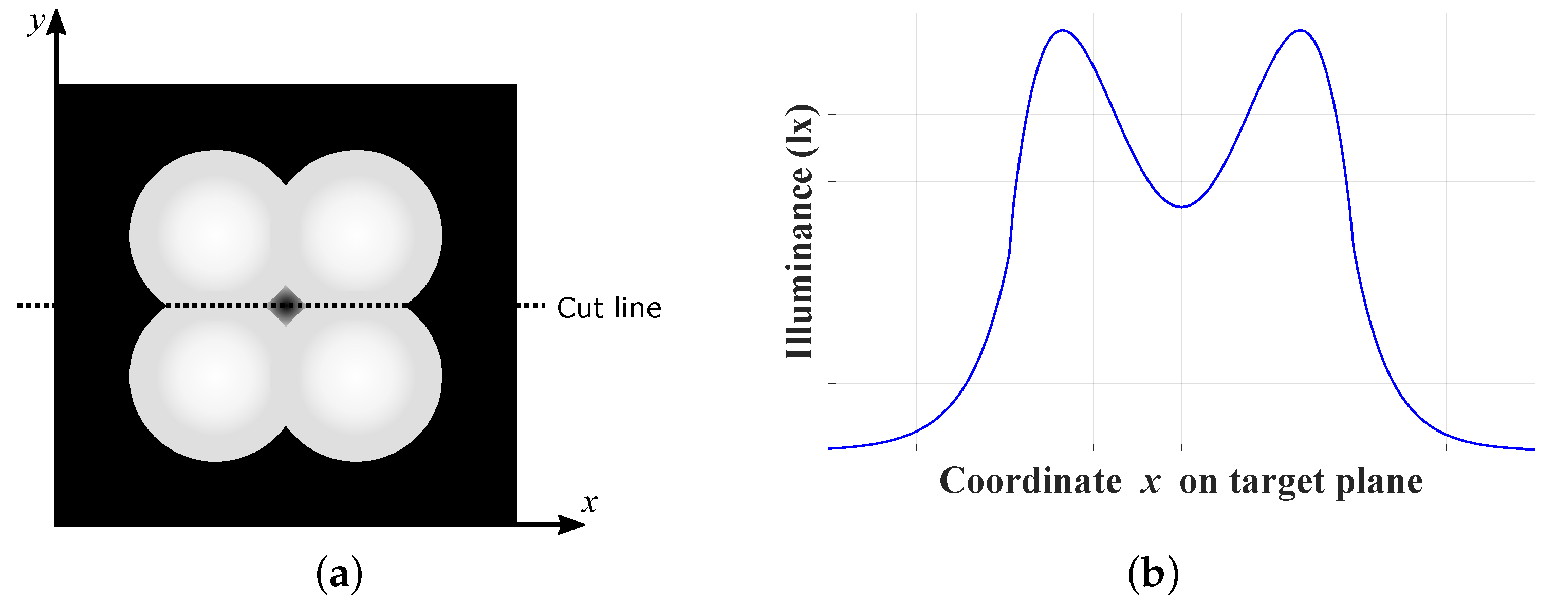
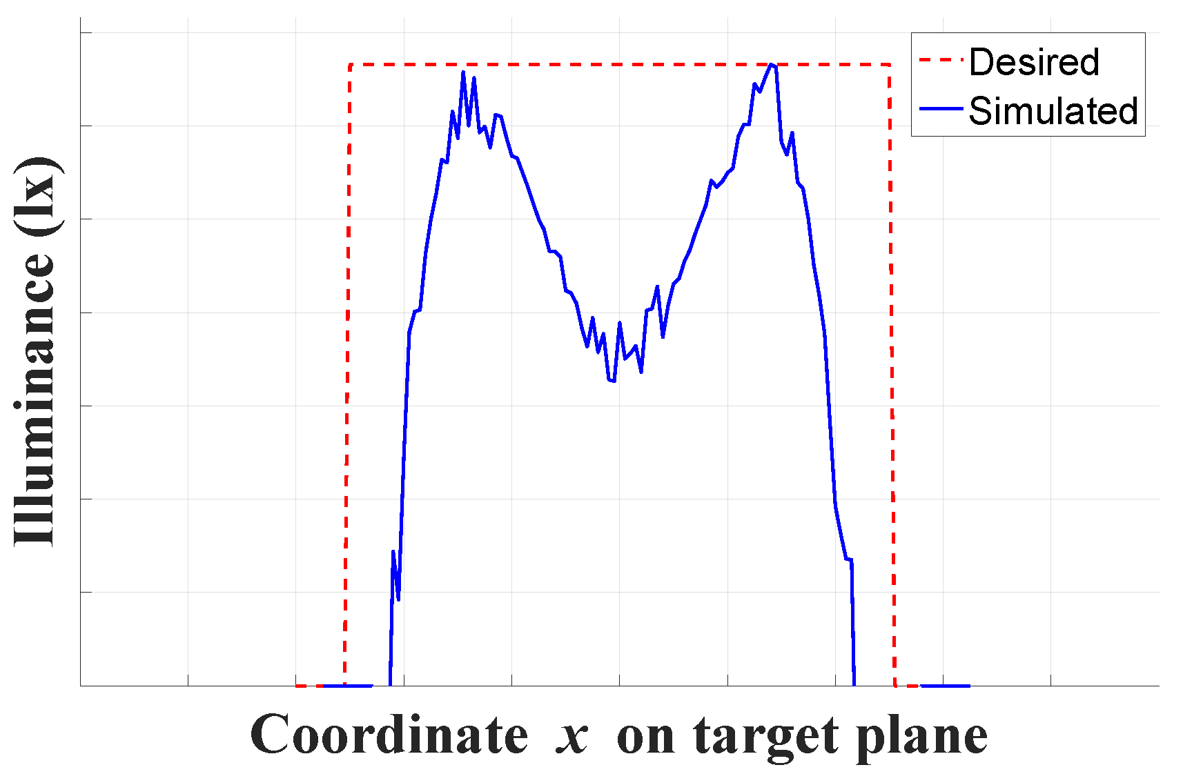
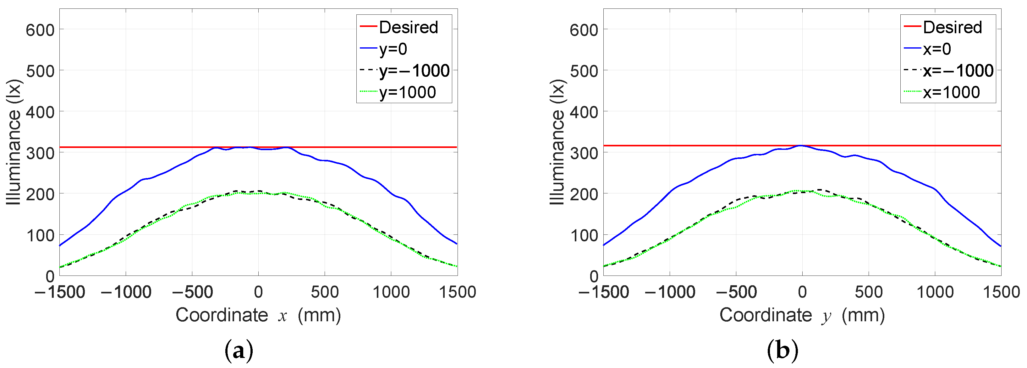
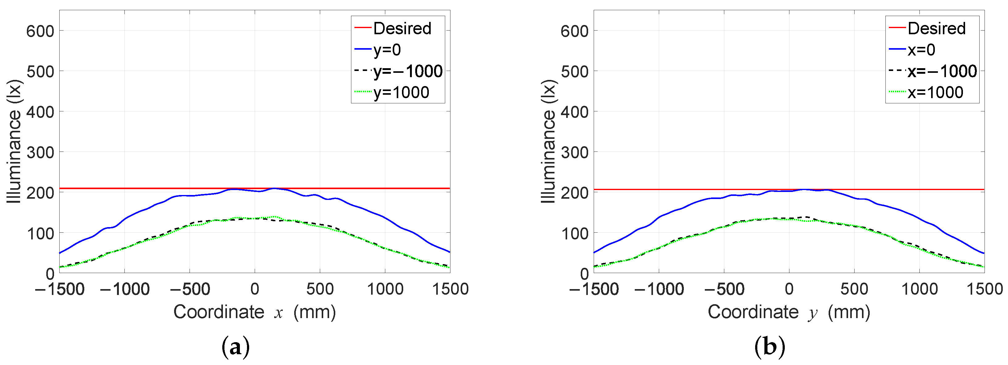
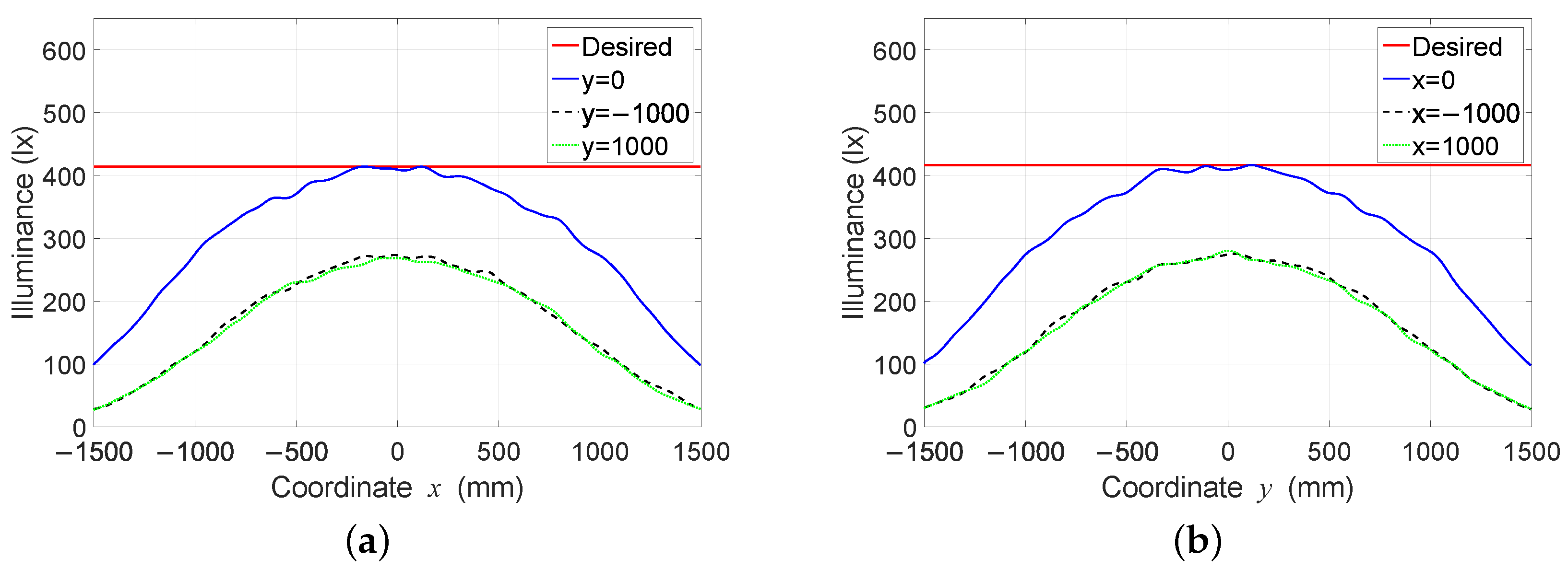
Figure 14a,b represent the illuminance on the target plane using the six verification profiles. This result is obtained by the solution found through the Quasi-Newton optimization technique in [46]. In this case, the optimized luminaire is composed of an array of $3\times 2$ HP-LED. Figure 15a,b are obtained by the optimized solution using the Nelder-Mead optimization technique, with an array of $4\times 2$ HP-LED. Comparing Figure 14 with Figure 15 there is an increase $\approx 100$ lx in the peak of illuminance obtained by the Nelder-Mead method, which possibly occurred due to the greater amount of LED.

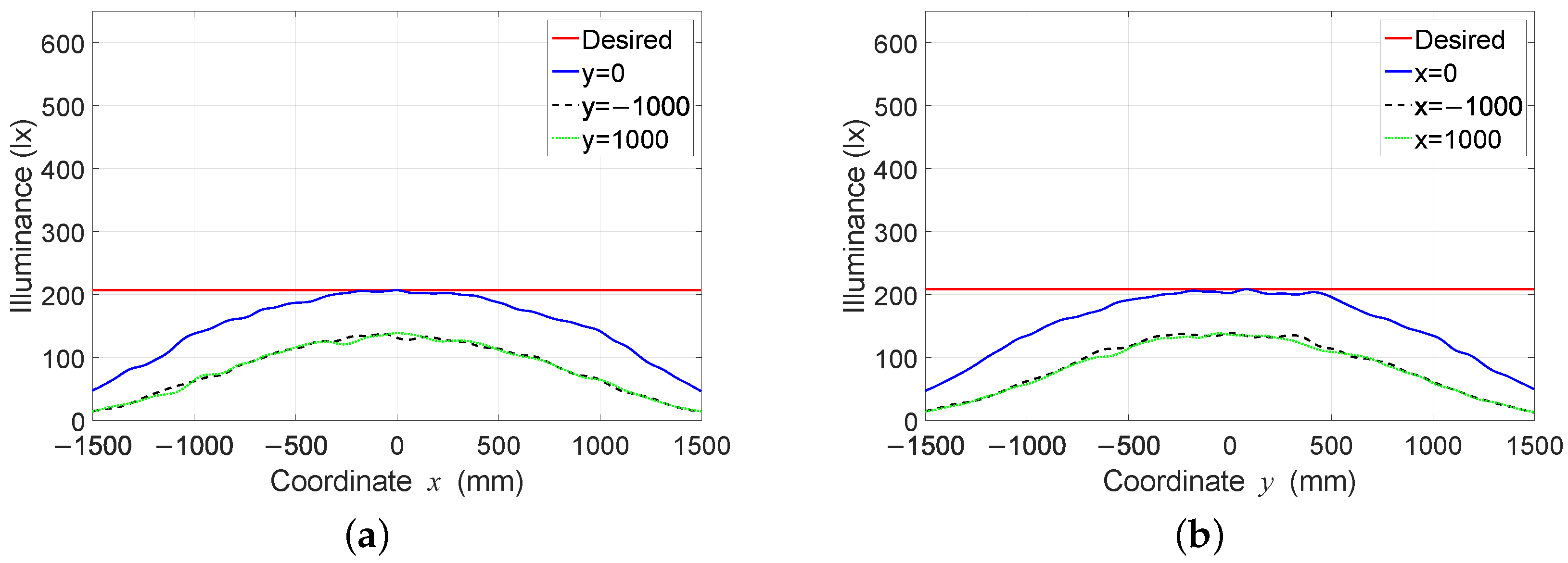
Figure 16a,b are results of the illuminance on the target plane obtained by the optimized luminaire using the BBO optimization technique with an array of $2\times 2$ HP-LED. Comparing the Figure 16 with Figure 15 it is possible to observe that there was a reduction in the illuminance peak in $\approx 200$ lx which is justified by the reduction in the number of HP-LEDs in the optimized arrangement. Thus, each pair of LEDs removed produces a $\approx 100$ lx reduction in the maximum illuminance value. Figure 17a,b represent the illuminance on the target plane of luminaire optimized through the genetic algorithm technique and reflects the result for the optimized arrangement of $2\times 2$ HP-LED. It is observed that there are no differences in the peak values of illuminance between the results in Figure 16 with Figure 17 obtained through the two heuristic techniques.

Each optimization method was simulated twice, once for the old evaluation function, published in [46] and another for the new evaluation function given by (8). To perform the comparison between the evaluation functions, the parameter $Tilt=0$ was considered in the evaluation function in (8). The values of $f\left(x\right)$ obtained through the new evaluation function in (8) and those obtained from the old evaluation function [46] are arranged in the

Table 4. Comparison between the evaluation function published in [46] and the new evaluation function in (8).

Algorithms	Evaluation Function	New Evaluation
	Published in [46]	Function (8)
Quasi-Newton	0.149	0.156
Nelder-Mead	0.2562	0.119
BBO	0.108	0.060
GA	0.105	0.060

. It is observed that in relation to the heuristic algorithms (genetic algorithm and BBO) the values found are the same and present a reduction of 50% in relation to the results of the deterministic algorithms. While in the old evaluation function [46] the genetic algorithm presents an approximate value to that of the BBO algorithm, due to the new evaluation function in (8), both reach the same value. On the other hand, the deterministic algorithms, in both evaluation functions, produce worse results than the heuristic algorithms, however, the solution obtained by the Nelder-Mead algorithm produces a better solution than the Quasi-Newton algorithm, when applying the new evaluation function.

The uniformity index U is calculated between two adjacent luminaires with the best case of $U=1$. Standards require specific values depending on each environment, purpose, and pedestrian and vehicle traffic. For external lighting cases, it is required $U\approx 0.2$. To measure the uniformity in the same luminaire, which is in addition to what is required by the standards, the uniformity index is computed for each case. Minimum and average illuminance are extracted to calculate the uniformity. They are obtained through the illuminance distribution curves of the three profiles on the coordinate axes x and y, generated in the simulation of a model parameterized by the proposed solution of the four optimization algorithms. The summary of these results, together with the values of minimum illuminance and average illuminance found, are displayed in

Table 5. Illuminance and uniformity ratio for the different optimization algorithms.

Algorithms	Illuminance	Illuminance	Uniformity (U)
	Minimum [lx]	Average [lx]
Quasi-Newton	19.86	160.32	0.124
Nelder-Mead	27.02	213.86	0.126
BBO	13.30	106.80	0.125
GA	12.96	106.98	0.121

.

In Table 5 it is observed that the average of the minimum illuminance found in the best results of the four algorithms was $18.28$ lx. In the case of the Nelder-Mead algorithm, the minimum illuminance is ≈50% greater than the mean illuminance, however, an increase in the mean illuminance value is also observed. Thus, the result of the ratio between the minimum value and the average value does not change. Therefore, the value of the uniformity index found for the four algorithms is approximately $0.12$ and the uniformity calculation method is unable to differentiate how uniform the illuminance is in the target plane for different lighting solutions. The initially proposed method of the evaluation function on a profile in [46], produces different results for each geometry obtained, as shown in Table 4.

4.3. Optimization Results Applying the New Methodology

To finalize the proposed methodology, the optimization process is performed considering all the changes proposed in this work, including the $Tilt$ parameter. The question to be answered is whether it is possible to obtain different and better results than the methodology adopted in Barbosa [46]. A summary of these results is displayed in

Table 6. Summary of optimization results.

Algorithm	$\overline{\mathit{f}}\left(\mathit{x}\right)$	U	m	n	Wh	Lh	Nf	Tilt
Quasi-Newton	0.135	0.123	3	2	175.8	57.0	5	1.0
Nelder-Mead	0.089	0.217	3	4	223.3	205.6	10	3.3
BBO	0.031	0.193	2	2	300.0	161.0	6	3.0
GA	0.027	0.228	2	2	300.0	300.0	4	2.1

, in which for each optimization algorithm technique applied, the value of the evaluation function $\overline{f}\left(x\right)$ is presented, the uniformity index U and the values of the six optimized luminaire geometry parameters.

In Table 6, it is observed that the solution found by the deterministic algorithms Quasi-Newton and Nelder-Mead obtained values of the $\overline{f}\left(x\right)$ better with the addition of the parameter $Tilt$, with a reduction of $14\%$ and $25\%$, respectively. Comparing the heuristic algorithms, a reduction of ≈50% in the value of $\overline{f}\left(x\right)$. In relation to the uniformity index, an increase was observed for all cases, which represents better results than those previously published in Barbosa [46]. It is verified that the genetic algorithm presented the best result among all the methods used for the optimization of the rectangular luminaire with $m\times n$ HP-LED. 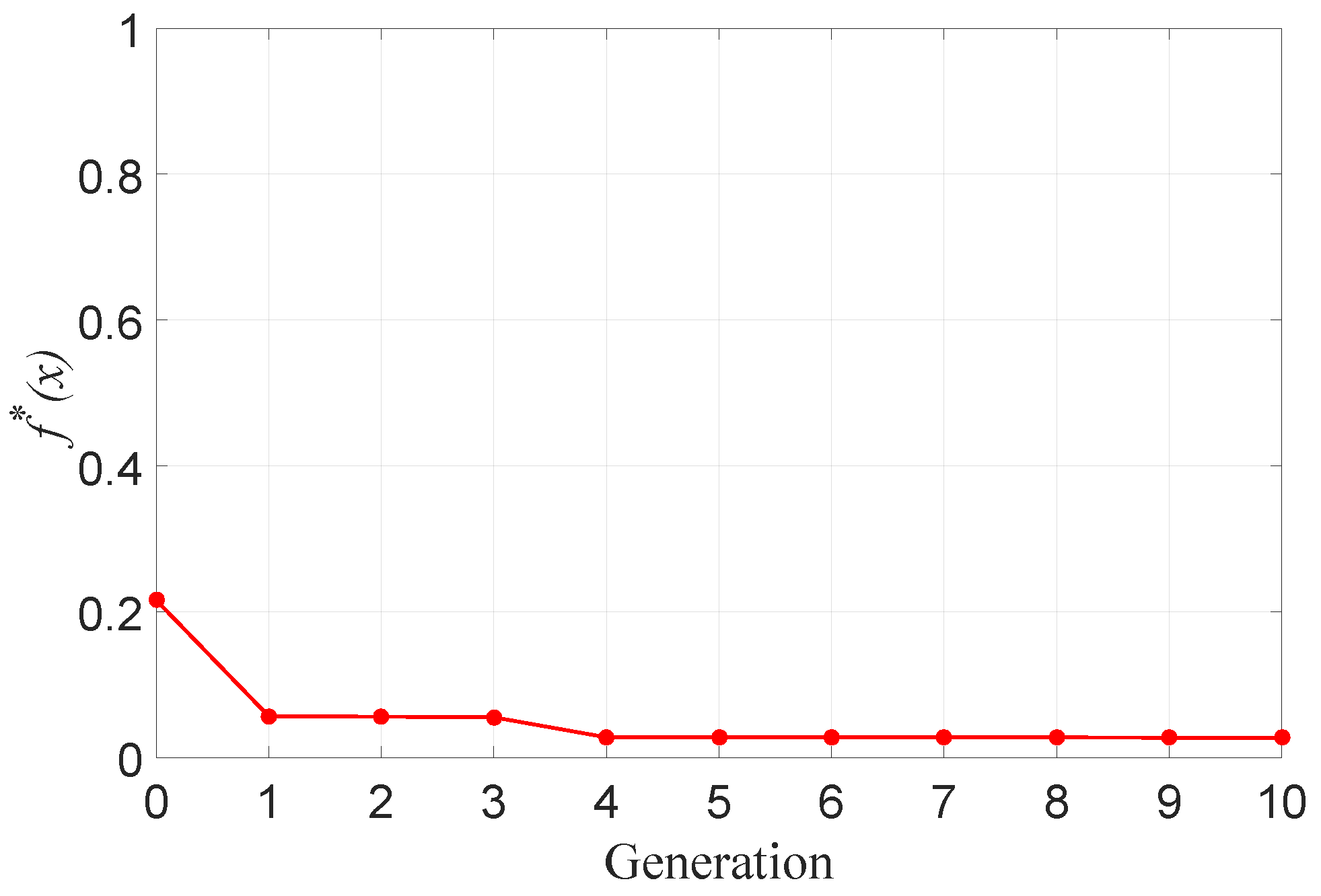Figure 18 shows the evolution of the value of $\overline{f}\left(x\right)$ across generations. The optimization was limited to ten generations with a population of 42 individuals. The computational time required to obtain the optimized solution was ≈54 h using a machine with an Intel Xeon 3.5Ghz board with twelve physical processors and 32 GB of RAM.

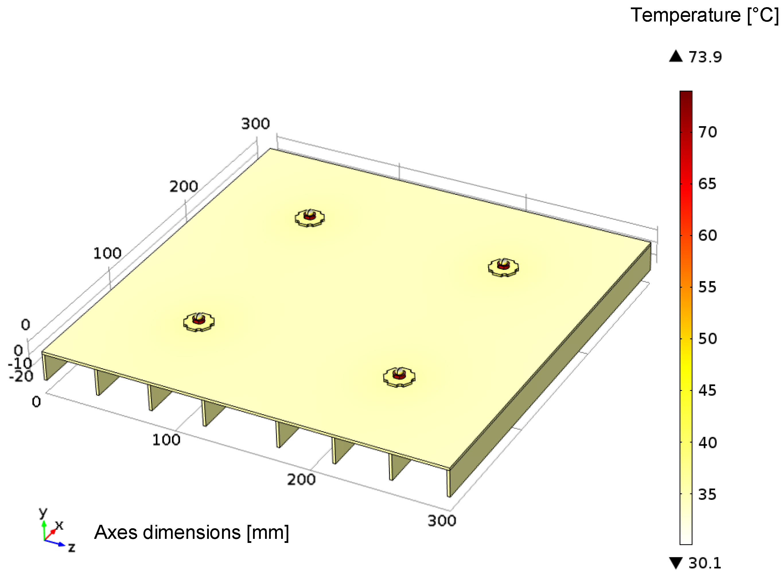
The optimized solution obtained proposes the design of a rectangular luminaire with an arrangement of $2\times 2$ HP-LED. Figure 19 presents the result of the optimized design of the HP-LED luminaire, as well as the heat distribution in a steady state. It is possible to see that the LED body is more reddish (warmer), representing higher temperatures. LED temperature in the simulation reaches a maximum value of $73.9$ ${}^{\circ }$C in a steady state, which is desired since temperatures above 120 ${}^{\circ }$C may damage the HP-LEDs. 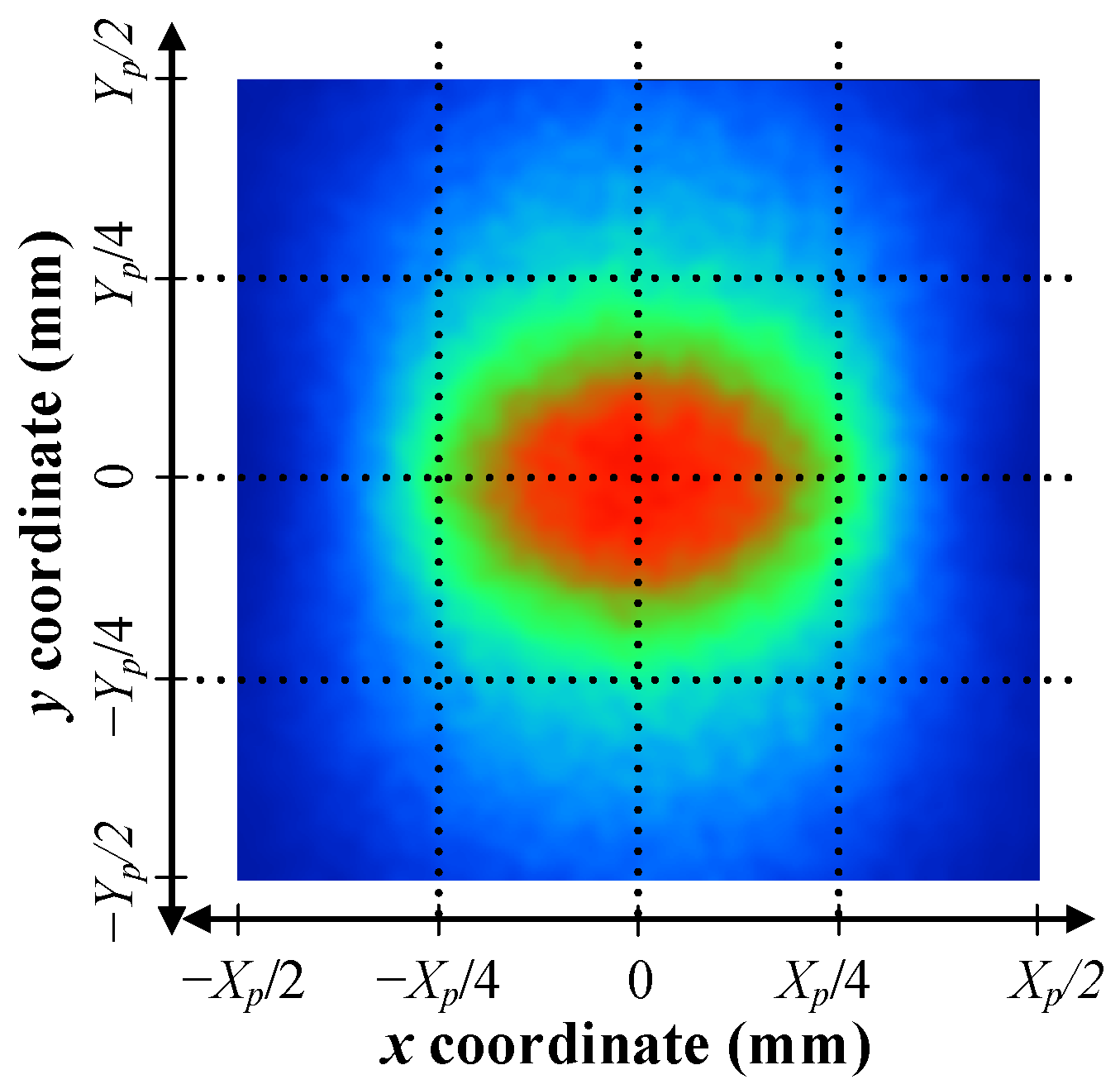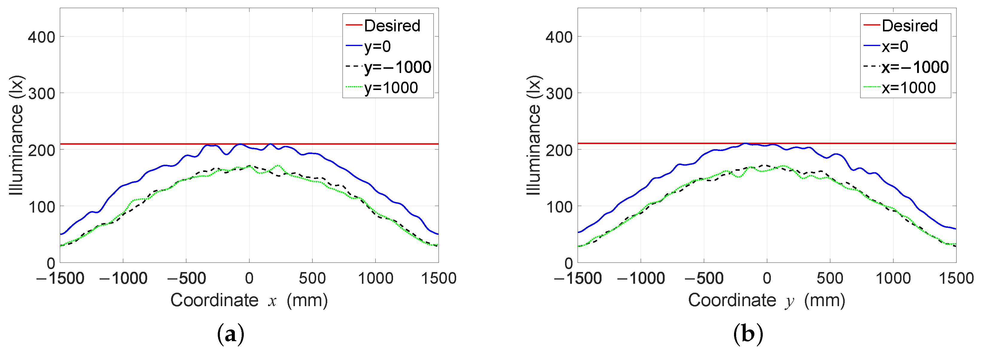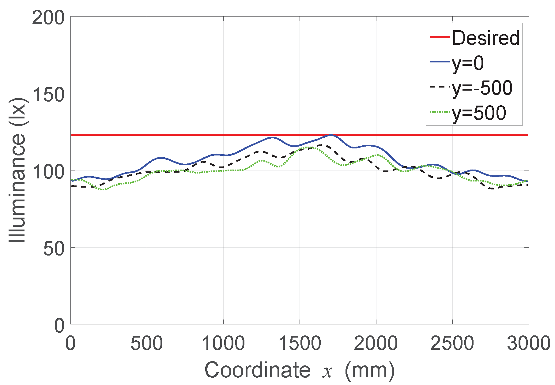Figure 20a presents the illuminance distribution curves for the GA-optimized solution on the coordinate axis x and Figure 20b on the coordinate axis y. To calculate the uniformity index, the lowest illuminance value in the six axes is found and the average illuminance value among all the values of the set is calculated.

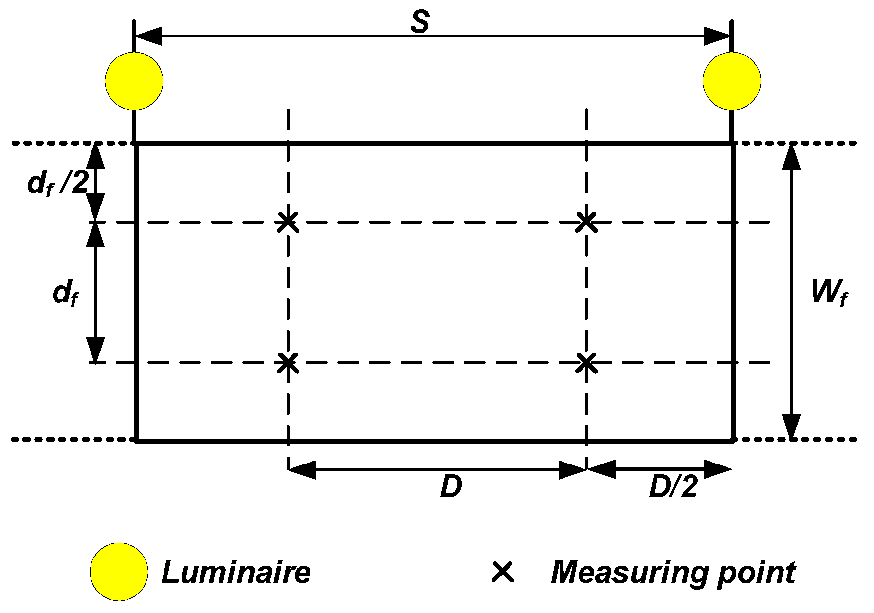
International standards establish a mesh of points on the target plane to measure uniformity in the lighting of external and internal environments. For work environments, it is recommended to measure the illuminance between nine and 36 points on the mesh. For public pedestrian or vehicular traffic lighting, a mesh is established consisting of fifteen measuring points arranged between two axes of luminaires. Another point that must be obeyed is the minimum horizontal illuminance value for each case and application. For the purpose of testing the validation of the results of the proposed methodology, the application of the luminaire for external area lighting is chosen, but precisely for the pedestrian way, with a sidewalk of $W_f=2$ m wide, distant sources of $S=3$ m, with axes located at the ends of the target plane. The lighting sources are suspended by 3 m high poles and a 1 m extension arm, so that they are centered under the road. With this perspective, the target plane illuminance distribution by two adjacent HP-LED optimized luminaires is analyzed. Figure 21 presents the illuminance distribution curves of the three profiles across the path (coordinate axis x) for the solution by genetic algorithm.

The overall uniformity index found is $0.8541$, with a minimum illuminance of $87.47$ lx, a maximum illuminance of $122.89$ lx and an average illuminance of $102.41$ lx. Standard EN 13201-2:2015, recommends average horizontal illuminance of 15 lx and minimum of 3 lx for the P1 (most critical) pedestrian street class. In this case, the minimum horizontal uniformity should be $0.3$. Therefore, the values obtained by the optimized luminaire meet the standard EN 13201-2:2015, and consequently other standards that were derived from it.

4.4. Discussion

Electricity demand is growing at a faster rate than the electricity production capacity. Energy efficiency in lighting not only reduces the gap between demand and production, but also includes other benefits such as the reduction of CO${}_2$ emitted in the process of energy consumption and thus helps to preserve the environment. HP-LEDs have emerged as an efficient and energy-efficient lighting alternative. Some of the technical challenges associated with using HP-LEDs are addressed in this document.

This work proposes to develop an optimization methodology for high-power LED luminaire projects that consider both thermal safety and luminous efficiency aspects. The evaluation function was developed in two parts, one considering the thermal study and the other considering the light study. In the light study, six uniformity evaluation profiles were proposed, three on the horizontal axis and three on the vertical axis that makes up the metric developed to position the solutions obtained. The optimized solution obtained by the genetic algorithm managed to obtain uniformity and illuminance index values higher than the minimum values recommended by the standards used.

In the proposed work, HP-LED lifespan is considered as indicated by the manufacturer, as long as the nominal specifications are maintained. This lifetime refers to the individual light source only and not to the entire luminaire. In the optimization process, the HP-LED lifespan was not taken into account, but rather the maintenance of the nominal specifications described by the manufacturer. If the nominal specifications are guaranteed, then the estimated lifespan is guaranteed.

As the market demands that LEDs have high brightness and small size, there is a contradiction between power density and operating temperature [30]. Thus, the P-N junction temperature of the HP-LED is directly related to the operating temperature of the lighting device. HP-LED lifespan is associated with their operating temperature and can be drastically reduced under high temperatures, which can even lead to permanent partial degradation or even total degradation. The thermal management challenge is to conduct heat from the LED chip to the environment at a sufficient heat transfer rate. The LED junction temperature is estimated through some techniques such as (i) from the LED module temperature and the LED junction thermal resistance, obtained from the manufacturer’s datasheet, (ii) through the derivation of the changes from the direct voltage on the component, and (iii) through direct measurements of the LED temperature via thermocouple sensor or infrared images [71,72]. Thus, the proposed methodology does not calculate the thermal uniformity of the LED junction temperature but limits the HP-LED temperature to a maximum value in the evaluation function. In the thermal simulation, it is possible to obtain the temperature value at the center of the LED and the thermal simulator was validated by a thermal camera.

Outdoor lighting is an extremely broad topic, covering roads, highways, tunnel lighting, traffic signs, parking, squares, sidewalks, paths dedicated to pedestrians, and others. Tomczuk’s et al. [73] work proposed unique lighting indexes for crosswalks as a reference. Five lighting classes are created, in which the recommended average horizontal illuminance ranges from 15 lx to 75 lx and the uniformity index is equal to $0.4$ for all classes. The need for new classes arises to fill the deficiency of the metrics normally used as references for a wide range of applications. The present work can be adapted for crosswalk applications, being a potential tool for comparing commercially existing solutions with projects obtained through optimized solutions.

Studies conducted by Boyce et al. [74] take into account the lighting of car parking lots in the USA and present a method for classifying safety and identifying the ideal illuminance. The results given suggest that the approximate average horizontal illuminance of 30 lx in a parking lot or sidewalk provides sufficient light to ensure safety perceptions. The initial results obtained in the present work indicate that the optimized luminaire design, in addition to meeting the minimum references presented in the standards, also meets specific studies such as the Boyce study et al. [74].

Wang et al. [14] presented numerical simulation results for average illuminance of $8.25$ lx and total uniformity of $0.364$. The proposed 80 W streetlight is comprised of a 5 W and 3 W LED combination in a target plan of 20 m × 10 m and a height of 8 m. The application of the luminaire is for secondary roads and no thermal analysis is performed on it. The analyzes presented in the present work are broader, contemplating both the light analysis and the thermal analysis. In this proposal, application-specific parameters can be adjusted for motorized roads.

Lo et al. [13] presented numerical simulation results for average illuminance of 14 lx and total uniformity of $0.37$. The proposed street light is 120 W composed of two LEDs clustered in a target plane of 30 m × 10 m and a height of 10 m. A similar study presented by Bender et al. [15] simulated in an 80 W luminaire with 30 LEDs achieved average illuminance results of 7 lx and total uniformity of $0.208$. Both studies are about applications on motorized roads and in both cases, lenses are used as an additional resource to the luminaire. In the first case, the values reached by the solution are too high due to the type of LED solution presented. In the present work, it appears that it is possible to achieve satisfactory results with lower financial and energy costs.

In the literature, most works focusing on illuminance and luminance indices talk about highways and crosswalks or cycle paths. There are few works that report studies and improvements in illuminance and luminance levels in pedestrian-only streets and promote the construction of a new metric to measure these indices. The present work innovates in creating a tool that allows the verification of uniformity for individual luminaires on the target plane. The widely used metrics only take into account the ratio between the minimum and average illuminance. The metric developed in this proposal is capable of evaluating lighting criteria and nominal thermal limitation criteria. In previous works published by the authors, both thermal and lighting simulations were validated by practical experiments. The present work presents an improvement in the optimization methodology and adds a new optimization technique for comparative effects.

5. Conclusions

The objective of this work was to develop an optimization methodology for the design of HP-LED luminaires that presented uniformity on the target plane according to references established by standards and adequate thermal management, ensuring luminous flux and useful life in the nominal standards of LEDs. A computational model of the geometry of the LED luminaire was also designed, thermal and optical analyzes were carried out through a simulator, and the luminaire geometry and the arrangement of the LED matrix were optimized, keeping the LED temperature below the maximum allowed values. In the proposal, the design of the luminaire can be used for internal or external lighting and can be applied in both cases with the necessary adaptations.

The process of optimizing HP-LED luminaire parameters is proposed and the tests are restricted to some heatsink designs and the LED array design. Optical accessories and cooling systems are not used in the optimization process, in an attempt to obtain a low-cost project. The results obtained are satisfactory when the values are compared with the standards. The proposed optimization process presented different luminaire geometries capable of improving the uniformity of the illuminance distribution on the target plane, without ceasing to be a thermally viable solution. In the results obtained, despite the deterministic methods reaching viable solutions, it was observed that they are strongly dependent on the seed. The heuristic methods achieved better performance with a lower amount of HP-LED, implying a lower initial and long-term financial cost, due to lower energy consumption.

The solution presented in this work was the best obtained, being able to compete with commercial models already existing in the market, however, adjustments are necessary for the domain restrictions initially defined. The luminaires currently sold do not have a lifetime study, maximum working temperature, or about luminous uniformity on the target plane. The methodology can be reproduced for the design of luminaires with a specific application, whether for internal or external environments, such as pedestrian circulation or vehicle traffic. To do so, the design domain constraints must be expanded and the simulation parameters defined according to the application, such as the height of the required lighting point.

Therefore, it is concluded that the metric currently used, which only considers the ratio between the minimum and average illuminance, is not efficient and cannot distinguish between different patterns of luminaire geometry which one has better uniformity in the distribution of the luminous flux. The metric developed in this proposal is capable of evaluating lighting criteria and nominal criteria for thermal limitation, even managing to classify different types of luminaires. For applications on roads with vehicular traffic, it should be considered that the recommendations on lighting quality defined in international standards also take into account luminance uniformity. The illuminance uniformity evaluates the brightness of the luminaire over a given region, while the luminance uniformity evaluates the brightness seen by the driver in the same region. Therefore, the evaluation of luminance uniformity is also necessary on roads with vehicular traffic.

Future research may include the construction of a prototype of the optimized solution found in this work with practical tests to validate the results obtained. It is also suggested the inclusion of new parameters for the luminaire design, such as those related to auxiliary optics to produce other desired lighting patterns in the target plane. Another suggestion would be to include in the evaluation function the verification of other requirements such as energy consumption of the luminaire, and total illuminance, among others.

References

1. Uchida, Y.; Taguchi, T. Lighting theory and luminous characteristics of white light-emitting diodes. Opt. Eng. 2005, 44, 124003. [Google Scholar] [CrossRef]
2. Navigant. Adoption of Light-Emitting Diodes in Common Lighting Applications: Snapshot of 2013 Trends; U.S. Department of Energy, Office of Energy Efficiency and Renewable Energy, Building Technologies Program: Washington, DC, USA, 2013.
3. Khan, M.N. Understanding LED Illumination; CRC Press: Boca Raton, FL, USA, 2013. [Google Scholar]
4. Martirano, L. A smart lighting control to save energy. In Proceedings of the 6th IEEE International Conference on Intelligent Data Acquisition and Advanced Computing Systems, Prague, Czech Republic, 15–17 September 2011; Volume 1. [Google Scholar]
5. Navigant. Energy Savings Forecast of Solid-State Lighting in General Illumination Applications; U.S. Department of Energy, Office of Energy Efficiency and Renewable Energy, Building Technologies Program: Washington, DC, USA, 2014.
6. Allouhi, A.; Fouih, Y.E.; Kousksou, T.; Jamil, A.; Zeraouli, Y.; Mourad, Y. Energy consumption and efficiency in buildings: Current status and future trends. J. Clean. Prod. 2015, 109, 118–130. [Google Scholar] [CrossRef]
7. Labeodan, T.; Bakkerb, C.D.; Rosemannb, A.; Zeiler, W. On the application of wireless sensors and actuators network in existing buildings for occupancy detection and occupancy-driven lighting control. Energy Build. 2016, 127, 75–83. [Google Scholar] [CrossRef] [Green Version]
8. Almeida, A.; Santos, B.; Paolo, B.; Quicheron, M. Renewable and Sustainable Energy Reviews; Elsevier: Amsterdam, The Netherlands, 2014; pp. 3430–3448. [Google Scholar]
9. Khan, T.Q.; Bodrogi, P.; Vinh, Q.T.; Winkler, H. (Eds.) LED Lighting: Technology and Perception; John Wiley & Sons: Weinheim, Germany, 2015. [Google Scholar]
10. Mottier, P. LED for Lighting Applications; John Wiley & Sons: Hoboken, NJ, USA, 2010; Volume 134. [Google Scholar]
11. Evans, D.L. High luminance LEDs replace incandescent lamps in new applications. In Proceedings of the SPIE 3002, Light-Emitting Diodes: Research, Manufacturing, and Applications, San Jose, CA, USA, 4 April 1997; pp. 142–153. [Google Scholar]
12. Barbosa, J.L.F.; Calixto, W.P.; Lima, R.A.; Alves, A.J.; Domingues, E.G. Thermal simulation and validation of 5 W high power LED luminaire. In Proceedings of the IEEE 15th International Conference on Environment and Electrical Engineering, Rome, Italy, 10–13 June 2015; pp. 2216–2220. [Google Scholar]
13. Lo, Y.-C.; Huang, K.-T.; Lee, X.-H.; Sun, C.-C. Optical design of a butterfly lens for a street light based on a double-cluster LED. Microelectron. Reliab. 2012, 52, 889–893. [Google Scholar] [CrossRef]
14. Wang, K.; Luo, X.; Liu, Z.; Zhou, B.; Gan, Z.; Liu, S. Optical analysis of an 80-W light-emitting-diode street lamp. Opt. Eng. 2008, 47, 013002. [Google Scholar] [CrossRef]
15. Bender, V.C.; Mendes, F.B.; Maggi, T.; Costa, M.A.D.; Marchesan, T.B. Design methodology for street lighting luminaires based on a photometrical analysis. In Proceedings of the 2013 Brazilian Power Electronics Conference, Gramado, Brazil, 27–31 October 2013; pp. 1160–1165. [Google Scholar]
16. Liu, P.; Wang, H.; Wu, R.; Yang, Y.; Zhang, Y.; Zheng, Z.; Li, H.; Liu, X. Uniform illumination design by configuration of LEDs and optimization of LED lens for large-scale color-mixing applications. Appl. Opt.-Opt. Soc. Am. 2013, 52, 3998–4005. [Google Scholar] [CrossRef]
17. Bai, K.; Wu, L.-G.; Nie, Q.-H.; Dai, S.-X.; Zhou, B.-Y.; Ma, X.-J.; Zheng, Z.-Y.; Zhang, F.-W. Thermal simulation and optimization of high-power white LED lamps. In Proceedings of the International Conference on Electronics, Communications and Control (ICECC), Ningbo, China, 9–11 September 2011; pp. 573–576. [Google Scholar]
18. Maaspuro, M.; Tuominen, A. Thermal analysis of LED spot lighting device operating in external natural or forced heat convection. Microelectron. Reliab. 2013, 53, 428–434. [Google Scholar] [CrossRef]
19. Chi, W.H.; Chou, T.-L.; Han, C.-N.; Yang, S.-Y.; Chiang, K.-N. Analysis of thermal and luminous performance of MR-16 LED lighting module. IEEE Trans. Compon. Packag. Technol. 2010, 33, 713–721. [Google Scholar] [CrossRef]
20. Bender, V.C.; Iaronka, O.; Costa, M.A.D.; Prado, R.N.; Marchesan, T.B. An optimized methodology for LED lighting systems designers. In Proceedings of the 2012 IEEE Industry Applications Society Annual Meeting, Las Vegas, NV, USA, 7–11 October 2012; pp. 1–8. [Google Scholar]
21. Bender, V.C.; Iaronka, O.; Marchesan, T.B. Study on the thermal performance of LED luminaire using finite element method. In Proceedings of the Industrial Electronics Society, IECON 2013-39th Annual Conference of the IEEE, Vienna, Austria, 10–13 November 2013; pp. 6099–6104. [Google Scholar]
22. Chang, M.-H.; Das, D.; Varde, P.V.; Pecht, M. Light emitting diodes reliability review. Microelectron. Reliab. 2012, 52, 762–782. [Google Scholar] [CrossRef]
23. Mura, G.; Vanzi, M. Reliability prediction and real world for LED lamps. In Proceedings of the IEEE 21st International Symposium on the Physical and Failure Analysis of Integrated Circuits (IPFA), Singapore, 30 June–4 July 2014; pp. 207–210. [Google Scholar]
24. Shailesh, K.R.; Kurian, C.P.; Kini, S.G.; Tanuja, S. Review of methods for reliability assessment of LED luminaires using optical and thermal measurements. In Proceedings of the International Conference on Green Computing, Communication and Conservation of Energy (ICGCE), Chennai, India, 2–14 December 2013; pp. 386–391. [Google Scholar]
25. Huaiyu, Y.; Koh, S.; van Zeijl, H.; Gielen, A.W.J.; Guoqi, Z. A review of passive thermal management of LED module. J. Semicond. 2011, 32, 014008. [Google Scholar]
26. Jakovenko, J.; Werkhoven, R.; Formánek, F.; Kunen, J.; Bolt, P.; Kulha, P. Thermal simulation and validation of 8W LED Lamp. In Proceedings of the 2011 12th International Conference on Thermal, Mechanical and Multi-Physics Simulation and Experiments in Microelectronics and Microsystems (EuroSimE), Linz, Austria, 17–20 April 2011; pp. 1/4–4/4. [Google Scholar]
27. Aoyama, Y.; Yachi, T. An LED module array system designed for streetlight use. In Proceedings of the IEEE Energy 2030 Conference, Atlanta, GA, USA, 17–18 November 2008; pp. 1–5. [Google Scholar]
28. Luo, X.; Cheng, T.; Xiong, W.; Gan, Z.; Liu, S. Thermal analysis of an 80 W light-emitting diode street lamp. IET Optoelectron. 2007, 1, 191–196. [Google Scholar] [CrossRef]
29. Christensen, T.V. Parallel Ray Tracing; Technical University of Denmark, Informatics and Mathematical Modelling: Kongens Lyngby, Denmark, 2009. [Google Scholar]
30. Luo, X.; Xiong, W.; Cheng, T.; Liu, S. Design and optimization of horizontally-located plate fin heat sink for high power LED street lamps. In Proceedings of the 2009 59th Electronic Components and Technology Conference, San Diego, CA, USA, 26–29 May 2009; pp. 854–859. [Google Scholar]
31. Scheepers, G.; Visser, J.A. Detailed thermal modeling of high powered LEDs. In Proceedings of the 2009 25th Annual IEEE Semiconductor Thermal Measurement and Management Symposium, San Jose, CA, USA, 15–19 March 2009; pp. 87–91. [Google Scholar]
32. Tang, H.; Li, D.; Pan, M.; Yang, T.; Yuan, C.; Fan, X. Thermal analysis and optimization design of LED streetlight module. In Proceedings of the 2013 10th China International Forum on Solid State Lighting (ChinaSSL), Beijing, China, 10–12 November 2013; pp. 193–197. [Google Scholar]
33. Jeong, M.W.; Jeon, S.W.; Kim, Y. Optimal thermal design of a horizontal fin heat sink with a modified-opening model mounted on an LED module. Appl. Therm. Eng. 2015, 91, 105–115. [Google Scholar] [CrossRef]
34. Luo, Y.; Feng, Z.; Han, Y.; Li, H. Design of compact and smooth free-form optical system with uniform illuminance for LED source. Opt. Express-Opt. Soc. Am. 2010, 18, 9055–9063. [Google Scholar] [CrossRef]
35. Feng, Z.; Luo, Y.; Han, Y. Design of LED freeform optical system for road lighting with high luminance/illuminance ratio. Opt. Express-Opt. Soc. Am. 2010, 18, 22020–22031. [Google Scholar] [CrossRef] [PubMed]
36. Jägerbrand, A.K. LED (Light-emitting diode) road lighting in practice: An evaluation of compliance with regulations and improvements for further energy savings. Energies 2016, 9, 357. [Google Scholar] [CrossRef] [Green Version]
37. Vasconcelos, L.E.M.; Limberger, M.A.C. Iluminação Eficiente: Iniciativas da Eletrobras Procel e Parceiros, 1st ed.; Eletrobras/Procel: Rio de Janeiro, Brazil, 2013. [Google Scholar]
38. Lenk, R.; Lenk, C. Practical lighting design with LEDs; John Wiley & Sons: Hoboken, NJ, USA, 2017. [Google Scholar]
39. Lasance, C.J.M.; Poppe, A. Thermal Management for LED Applications; Springer: New York, NY, USA, 2014; Volume 2. [Google Scholar]
40. Liu, S.; Luo, X. LED Packaging for Lighting Applications: Design, Manufacturing, and Testing; John Wiley & Sons: Hoboken, NJ, USA, 2011. [Google Scholar]
41. Couldwell, C. Multi-Die Packages versus Multiple Single Die Power LEDs; Electronics Weekly.com: Croydon, UK, 2008; pp. 1–13. [Google Scholar]
42. Hsu, C.N.; Wang, W.C.; Fang, S.H. Experimental of ultra-high-power multichip COB LED. J. Therm. Anal. Calorim. 2019, 136, 2097–2109. [Google Scholar] [CrossRef]
43. Keppens, A. Modelling and Evaluation of High-Power Light-Emitting Diodes for General Lighting; KU Leuven University Press: Leuven, Belgium, 2010. [Google Scholar]
44. US-DOE. Annual Energy Outlook 2015 with Projections to 2040; US Energy Information Administration: Washington, DC, USA, 2015.
45. Veitch, J.A.; Newsham, G.R. Lighting Quality and Energy-Efficiency Effects on Task Performance, Mood, Health, Satisfaction, and Comfort. J. Illum. Eng. Soc. 1998, 27, 107–129. [Google Scholar] [CrossRef]
46. Barbosa, J.L.F.; Simon, D.; Calixto, W.P. Design Optimization of a High Power LED Matrix Luminaire. Energies 2017, 10, 639. [Google Scholar] [CrossRef] [Green Version]
47. Jennic. Intelligent Street Lighting; Jennic Ltd.: Hong Kong, China, 2009. [Google Scholar]
48. Shakhmatova, K. A History of Street Lighting in the Old and New Towns of Edinburgh World Heritage Site; Edinburgh World Heritage: Edinburgh, UK, 2011. [Google Scholar]
49. HYDROQUEBEC. Comparison Of Electricity Prices in Major North American Cities 2011; Bibliothèque et Archives nationales du Québec: Montréal, QC, Canada, 2011. [Google Scholar]
50. Barbosa, J.L.F. Metodologia de Otimização de Lentes para Lâmpadas de LED. Master’s Thesis, Universidade Federal de Goiás, Goiânia, Brazil, 2013. [Google Scholar]
51. Borbely, A.; Johnson, S.G. Prediction of light extraction efficiency of LEDs by ray trace simulation. Third Int. Conf. Solid State Light. 2004, 5187, 301–308. [Google Scholar]
52. Hantschel, T.; Kauerauf, A.I.; Wygrala, B. Finite element analysis and ray tracing modeling of petroleum migration. Mar. Pet. Geol. Elsevier 2000, 17, 815–820. [Google Scholar] [CrossRef]
53. Campos, R.M. Simulação da Transferência de Calor em Processos de Soldagem 3D Utilizando o Método dos Elementos de Contorno. Master’s Thesis, Departamento de Engenharia Mecânica, Faculdade de Tecnologia, Universidade de Brasilia, Brasilia, Brazil, 2012. [Google Scholar]
54. Petropoulos, G.P.; Ireland, G.; Griffiths, H.M.; Kennedy, M.C.; Ioannou-Katidis, P.; Kalivas, D.P. Extending the Global Sensitivity Analysis of the SimSphere model in the Context of its Future Exploitation by the Scientific Community. Water 2015, 7, 2101–2141. [Google Scholar] [CrossRef] [Green Version]
55. Gomes, V.M. Complexidade Natural de Sistemas Baseada em Análise de Sensibilidade. Ph.D. Thesis, Escola de Engenharia Elétrica, Mecânica e de Computação, Universidade Federal de Goias—UFG, Goiânia, Brazil, 2020. [Google Scholar]
56. Frey, C.H.; Patil, S.R. Identification and Review of Sensitivity Analysis Methods: Risk Analysis; Wiley Online Library: Hoboken, NJ, USA, 2002; Volume 22, pp. 553–578. [Google Scholar]
57. Lima, R.A. Metodologia para Simulação e Otimização em Problemas de Análise Eletromagnética. Ph.D. Thesis, Escola de Engenharia Elétrica, Mecânica e de Computação, Universidade Federal de Goias—UFG, Goiânia, Brazil, 2020. [Google Scholar]
58. Eschenbach, T.G.; McKeague, L.S. Exposition on using graphs for sensitivity analysis. Eng. Econ. 1989, 34, 315–333. [Google Scholar] [CrossRef]
59. Saraiva, J.P.; Lima, B.S.; Gomes, V.M.; Flores, P.H.R.; Gomes, F.A.; Assis, A.O.; Reis, M.R.C.; Araujo, W.R.H.; Abrenhosa, C.; Calixto, W.P. Calculation of sensitivity index using one-at-a-time measures based on graphical analysis. In Proceedings of the 2017 18th International Scientific Conference on Electric Power Engineering (EPE), Ostrava, Czech Republic, 17–19 May 2017; pp. 1–6. [Google Scholar]
60. Santos, J.M.M.; Augusta, S. Métodos computacionais de otimização. In Proceedings of the Colóquio Brasileiro de Matemática, Rio de Janeiro, Brazil, 24–28 July 1995; Volume 20. [Google Scholar]
61. Rios, L.M.; Sahinidis, N.V. Derivative-free optimization: A review of algorithms and comparison of software implementations. J. Glob. Optim. 2011, 56, 1247–1293. [Google Scholar] [CrossRef] [Green Version]
62. Simon, D. Biogeography-based optimization. Trans. Evol. Comput. 2008, 12, 702–713. [Google Scholar] [CrossRef] [Green Version]
63. Ma, H.; Simon, D.; Siarry, P.; Yang, Z.; Fei, M. Biogeography-based optimization: A 10-year review. IEEE Trans. Emerg. Top. Comput. Intell. 2017, 1, 391–407. [Google Scholar] [CrossRef]
64. Simon, D. Evolutionary Optimization Algorithms; John Wiley & Sons: Hoboken, NJ, USA, 2013. [Google Scholar]
65. Linden, R. Algoritmos Geneticos; Brasport: La Chaux-de-Fonds, Switzerland, 2006. [Google Scholar]
66. Sivanandam, S.N.; Deepa, S.N. Introduction to Genetic Algorithms; Springer Publishing Company, Incorporated: Berlin/Heidelberg, Germany, 2007. [Google Scholar]
67. Michalewicz, Z.; Fogel, D. How to Solve It: Modern Heuristics; Springer: Berlin/Heidelberg, Germany, 2000. [Google Scholar]
68. Barbosa, J.L.F.; Alves, A.J.; Barbosa, A.C.O.F.; Ferraz, R.S.; Calixto, W.P. Lighting Simulation and Validation for High Power LED Matrix Luminaire. In Proceedings of the 2018 IEEE International Conference on Environment and Electrical Engineering and 2018 IEEE Industrial and Commercial Power Systems Europe (EEEIC/I&CPS Europe), Palermo, Italy, 12–15 June 2018; pp. 1–4. [Google Scholar]
69. COMSOL Multiphysics. Heat Transfer Module User’s Guide; COMSOL Version 4.4; Comsol AB Group: Stockholm, Sweden, 2013. [Google Scholar]
70. ZEMAX Optical Design Program User’s Guide; Focus Software, Inc.: Tucson, Arizona, 2002; 561p.
71. Pryde, J.R. Methods of determining LED operating junction temperature experimental and theoretical. LED Prof. Rev. Luger Res. eU 2012, 32, 42–48. [Google Scholar]
72. Tsai, M.Y.; Chen, C.H.; Kang, C.S. Thermal measurements and analyses of low-cost high-power LED packages and their modules. Microelectron. Reliab. 2012, 52, 845–854. [Google Scholar] [CrossRef]
73. Tomczuk, P.; Jamroz, K.; Mackun, T.; Chrzanowicz, M. Lighting requirements for pedestrian crossings—Positive contrast. MATEC Web Conf. 2019, 262, 05015. [Google Scholar] [CrossRef]
74. Boyce, P.R.; Eklund, N.H.; Hamilton, B.J.; Bruno, L.D. Perceptions of safety at night in different lighting conditions. Int. J. Light. Res. Technol. 2000, 32, 79–91. [Google Scholar] [CrossRef]
Figure 1. Distribution of world electricity consumption by sectors.
Energies 15 07679 g001
Figure 2. Flowchart of the Quasi-Newton method.
Energies 15 07679 g002
Figure 3. Flowchart of the Nelder-Mead method.
Energies 15 07679 g003
Figure 4. Flowchart of BBO method.
Energies 15 07679 g004
Figure 5. Flowchart of GA method.
Energies 15 07679 g005
Figure 6. Hypothetical illustration of the m × n matrix arrangement on rectangular luminaire.
Energies 15 07679 g006
Figure 7. Geometric parameters referring to heat dissipation: (a) 3D model and (b) 2D model.
Energies 15 07679 g007
Figure 8. Hypothetical illustration of a luminaire with four LEDs: (a) HP-LED radiation pattern on the target plane and (b) values of illuminance on the cut line on the x axis.
Energies 15 07679 g008
Figure 9. Evaluation function suggested in Barbosa [50].
Energies 15 07679 g009
Figure 10. Hypothetical illuminance in the target plane of X P × Y P with 3 linear profiles on each axis.
Energies 15 07679 g010
Figure 11. Proposed temperature evaluation function.
Energies 15 07679 g011
Figure 12. Reticulated mesh for illuminance measurement.
Energies 15 07679 g012
Figure 13. New temperature evaluation function proposal.
Energies 15 07679 g013
Figure 14. Illuminance distribution curves of the three profiles found using the Quasi-Newton optimization algorithm: (a) on the coordinate axis x and (b) on the coordinate axis y.
Energies 15 07679 g014
Figure 15. Illuminance distribution curves of the three profiles found using the Nelder-Mead optimization algorithm: (a) on the coordinate axis x and (b) on the coordinate axis y.
Energies 15 07679 g015
Figure 16. Illuminance distribution curves of the three profiles found using the BBO optimization algorithm: (a) on the coordinate axis x and (b) on the coordinate axis y.
Energies 15 07679 g016
Figure 17. Illuminance distribution curves of the three profiles found using genetic algorithm: (a) on the coordinate axis x and (b) on the coordinate axis y.
Energies 15 07679 g017
Figure 18. Value of the evaluation function × generation of the genetic algorithm.
Energies 15 07679 g018
Figure 19. HP-LED luminaire surface temperature for the result optimized by genetic algorithm.
Energies 15 07679 g019
Figure 20. Illuminance distribution curves of the three profiles found using genetic algorithm: (a) on the coordinate axis x and (b) on the coordinate axis y.
Energies 15 07679 g020
Figure 21. Illuminance distribution curves of two adjacent lighting points generated by the GA-optimized solution.
Energies 15 07679 g021