Sensorless Control of High-Speed Motors Subject to Iron Loss

Abstract

It is widely recognized that the iron loss produced by motors at high speeds will directly affect the angle and size of the back electromotive force, and, therefore, it cannot be ignored. In this paper, a high-performance sensorless control algorithm is proposed for high-speed permanent magnet synchronous motors (HSPMSM), taking the iron loss into account. First, the resistance representing the core loss is precalculated by finite element analysis, and then a sliding mode observer with disturbance observation is designed to estimate the rotor position. The observer possesses the advantages of suppressing the chattering phenomenon and enhancing the robustness against uncertainty. Meanwhile, the idea of the characteristic model is used to design an adaptive robust control law to improve the speed control accuracy. Subsequently, a sensorless control scheme is proposed by using the proposed observer in combination with the designed control scheme. The stability of the observer and controller is verified by the Lyapunov theory method. Finally, a simulation example is given to demonstrate the correctness and the effectiveness of the proposed algorithm.

1. Introduction

Nowadays, high-speed permanent magnet synchronous motors have been widely used in many industrial applications that demand a high precision with good efficiency, such as numerical control machines, electric vehicles and robots [1,2]. The vector control strategy, which is extensively used in the control of motors, requires mechanical sensors such as encoders to provide position information. However, the deployment of sensors will inevitably lead to hardware consumption, reliability reduction and cost increases [3]. Moreover, at high speeds, it is very sensitive to environmental variations such as vibration and temperature. As such, many scholars at home and abroad have carried out a lot of fruitful research work on the sensorless control theory and technology, aiming to accurately estimate the speed and position of the rotor through appropriate methods by using the relevant electrical signals of the motor windings so as to replace the mechanical sensors.

The sliding mode control technique has many advantages, such as insensitivity to structural uncertainty, a strong robustness against disturbances and a fast dynamic response, but this method has inherent chattering problems. In [4], a low-pass filter and additional position compensation of the rotor were used to reduce chattering problems. In [5], in order to improve the observation accuracy and robustness of the sensorless control of a permanent magnet synchronous motor, an over-twist algorithm based on adaptive parameter estimation control was proposed, which had an integral effect on the switching function, effectively improved the convergence speed of the system and enhanced the observation accuracy of the rotor position and speed. In [6], a sliding mode observer based on a two-stage filter was designed. The output of the first-stage filter provides a feedback observer for the current. The rotor position is calculated by using the output of the second-stage filter, and the position estimation error is compensated by piecewise linear compensation. In [7], the saturation function was replaced by the sign function to weaken the chattering. In addition, the steady-state performance of the sliding mode observer was improved by estimating the variations of stator resistance. In [8], a high-gain observer was used to estimate the state under scalar disturbance. In [9], an adaptive sliding mode observer combined with back electromotive force error estimation was proposed to reduce system chattering.

In the above-mentioned sensorless method, the iron loss of the motor is ignored. However, in the high-speed area, the effects resulting from iron loss cannot be simply ignored, as it increases to the square of the speed [10]. In [11], a sensorless drive control based on a disturbance observer that accurately estimates the rotor position was proposed. This is achieved by considering the iron loss so as to further reduce the rotor position estimation error. In reference [12], a sensorless control strategy of permanent magnet synchronous motors based on high-frequency switching voltage injection was proposed, which considers the loss of iron and compensates it. In reference [13], a sliding mode observer was designed for the iron loss model of the motor, and the recursive least square method was used to estimate the motor parameters and iron loss resistance. The sensorless control methods above only consider the variation in iron loss resistance or some system parameters and consider the other parameters to be constants. In fact, the parameters of flux linkage, resistance, inductance, etc. will vary with environmental factors. Therefore, for the HSPMSM observer designs, it is desirable to deal with parameter variations and unknown uncertainties simultaneously.

In order to improve the tracking performance and robustness of the nonlinear system, many advanced nonlinear controllers have been proposed, such as internal model control [14], feedback linearization control [15], combined direct and indirect approaches to adaptive control [16], adaptive backstepping control [17], etc. In [18], Cecati et al. proposed a passivity-based control for induction motors. The reference position was reached very quickly and without overshoot and was maintained with a high precision, even when load changes and parameter variations occurred. Yao bin et al. proposed an adaptive robust control (ARC) [19] method and successfully applied it to multiple systems [20,21,22]. These controllers ensure the transient performance and final tracking accuracy of the given output tracking and achieve asymptotic output tracking without unstructured uncertainties.

However, all of the above-mentioned nonlinear methods adopt the full-state feedback method, where the position and velocity signals must be measured at least. It should be pointed out that, for many systems, due to the cost reduction or the inconvenience of system detection, only input and output signals are available. In addition, a large amount of measurement noise may reduce the realizable performance of the full-state feedback controller. Although some system states can also be estimated by state observers [23], when the system order is relatively high, the backstepping control scheme needs to identify more parameters, and the number of the intermediate virtual control rate will also increase rapidly, which makes the controller structure very complex and not conducive to engineering applications.

The academician Wu put forward the idea of characteristic modeling in the 1990s [24]. The characteristic model compresses the high-order or uncertain terms of the complex object into several time-varying characteristic parameters without losing the information of the object, but the description form is very simple. The characteristic model provides the basis for the design of low-order controllers for the high-order complex object, which is convenient for the design of controllers and easy for engineering applications [25]. Reference [26] extended the characteristic modeling method to the gear-driven servo system with inertia change, which reduced the complexity of the traditional mathematical model, and the designed second-order terminal sliding mode controller achieved good results. In reference [27], by combining characteristic modeling, a genetic algorithm and terminal sliding mode control, an adaptive discrete terminal sliding mode controller based on a characteristic model was proposed, which can not only enhance the robustness of the system but also eliminate the chattering effect of system commutation. The above-mentioned control methods use characteristic modeling to simplify the controller design and have achieved good control results. The characteristic model solves the problem of it being difficult to accurately model the complex system and design the controller, which provides a good reference for the modeling and controller design of high-performance high-speed motor control systems.

This paper presents a sensorless control method of high-speed permanent magnet synchronous motors (HSPMSM) that considers iron loss, which can achieve a good speed tracking control performance under high-speed operation. The main contributions of this paper are as follows: first, the iron loss in the motor system is obtained by using finite element analysis, and the change relationship of iron loss resistance, inductance and flux linkage is included in a lookup table to overcome the influence of iron loss on sensorless control. Second, a disturbance observer is added to the observer to deal with the influence of unknown disturbances on the system, and the arctangent function is used to replace the saturation function in the traditional sliding mode control to reduce chattering. Third, an adaptive robust control method based on a characteristic model is designed. The characteristic model is used to describe the high-speed permanent magnet synchronous motor, which solves the problem of the control system model being complex and difficult to describe accurately. The adaptive robust controller that is designed based on the characteristic model can deal with parameter uncertainty and unknown disturbance simultaneously, which improves the control accuracy and robustness of the system.

This paper is organized as follows. The model and sensorless control of HPMSM are presented in Section 2. Section 3 shows the design of the adaptive robust controller based on the characteristic model and its main theoretical results. Section 4 provides the simulation results. Some conclusions can be found in Section 5.

2. Model and Sensorless Control of HPMSM

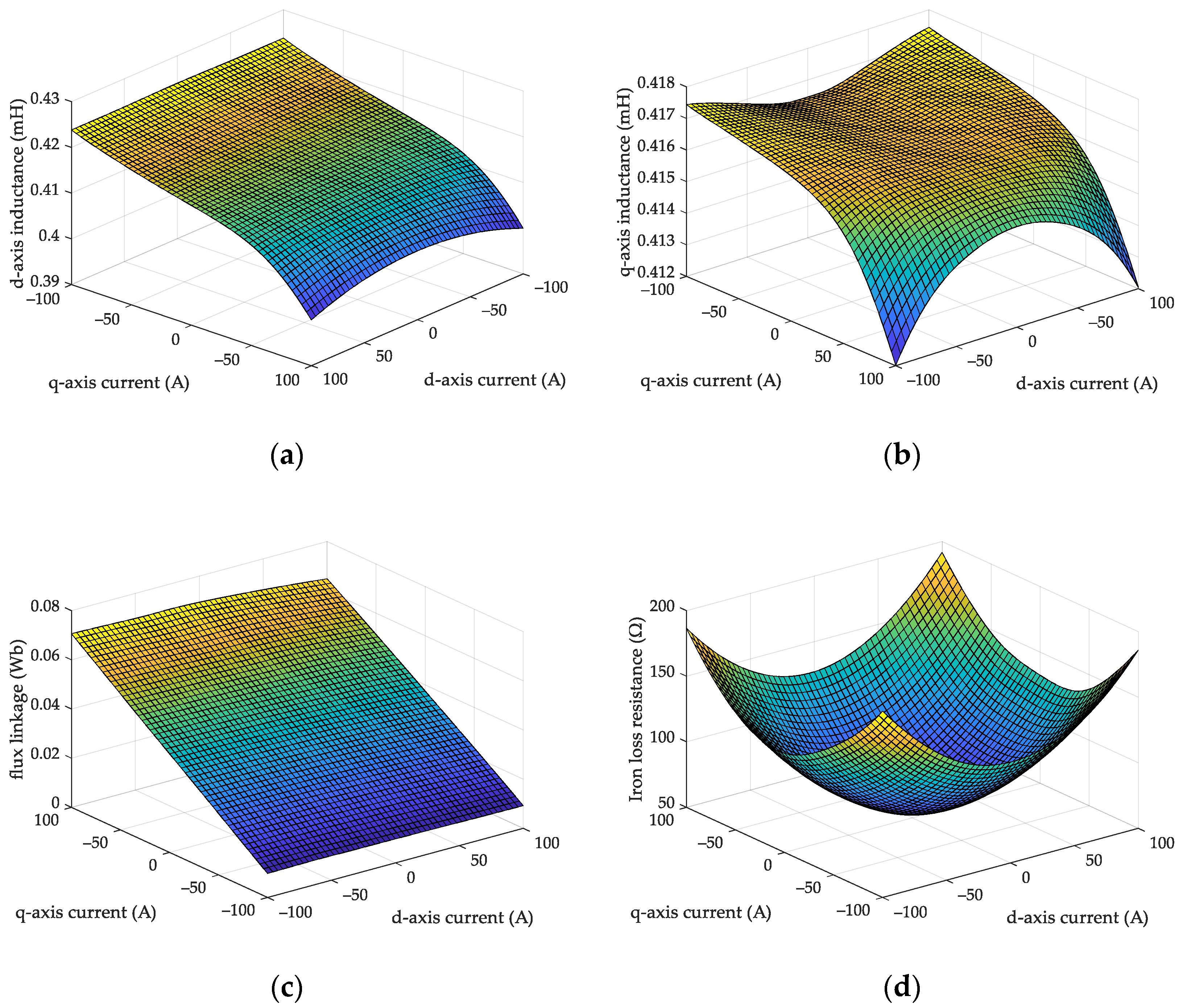
2.1. Model of HSPMSM with Iron Loss

After the core loss is introduced into the HSPMSM model, its equivalent circuit is shown in Figure 1.

Based on the above equivalent circuit, the mathematical model of HSPMSM considering iron loss can be obtained [2,28]:

$$\left[\begin{array}{l}{u}_{\mathrm{d}}\\ u_{\mathrm{q}}\end{array}\right]=\left[\begin{array}{cc}{R}_{\mathrm{m}}+p{L}_{\mathrm{d}}& -{\omega }_{\mathrm{e}}{L}_{\mathrm{q}}+p\frac{{\omega }_{\mathrm{e}}{L}_{\mathrm{d}}{L}_{\mathrm{q}}}{R_{\mathrm{i}}}\\ {\omega }_{\mathrm{e}}{L}_{\mathrm{d}}-p\frac{{\omega }_{\mathrm{e}}{L}_{\mathrm{d}}{L}_{\mathrm{q}}}{R_{\mathrm{i}}}& R_{\mathrm{m}}+p{L}_{\mathrm{q}}\end{array}\right]\left[\begin{array}{l}{i}_{\mathrm{d}}\\ i_{\mathrm{q}}\end{array}\right]+\left[\begin{array}{l}\frac{{\omega }_{\mathrm{e}}^2{L}_{\mathrm{q}}{\psi }_{\mathrm{f}}}{R_{\mathrm{i}}}\\ {\omega }_{\mathrm{e}}{\psi }_{\mathrm{f}}\end{array}\right],$$

(1)

where $i_{\mathrm{d}}$ and $i_{\mathrm{q}}$ are the currents of the d-q axis; $u_{\mathrm{d}}$ and $u_{\mathrm{q}}$ are the voltage of the d-q axis; $p=d/(dt)$ is the differential; $R_{\mathrm{m}}=R_{\mathrm{s}}+(({\omega }_{\mathrm{e}}^2{L}_{\mathrm{d}}{L}_{\mathrm{q}})/R_{\mathrm{i}})$; $R_{\mathrm{s}}$ is the stator resistance; ${\psi }_{\mathrm{f}}$ is the flux linkage of the permanent magnet; $R_{\mathrm{i}}$ is the equivalent resistance of iron loss; $L_{\mathrm{d}}$ and $L_{\mathrm{q}}$ are the inductance of the d-q axis; ${\omega }_{\mathrm{e}}$ is the speed.

In order to obtain the relevant motor parameters in the motor model, the electromagnetic field finite element method is used for the numerical analysis of the motor electromagnetic field, and

Table 1. Parameters of the simulation model.

pole	1
number of conductors per slot	8
number of parallel branches	2
inner diameter of stator	70 mm
outer diameter of stator	130 mm
inner diameter of rotor	15 mm
outer diameter of rotor	64 mm
length of iron core	130 mm

lists the design parameters of the tested motor.

The nonlinear relationship of motor parameters with respect to the d-q axis current component is shown in Figure 2.

2.2. Design of the Sliding Mode Observer

According to Equation (1), the dynamic equation of the stator current is rewritten as

$${\dot{i}}_{\mathrm{dq}}=\mathrm{A}{i}_{\mathrm{dq}}+\mathrm{B}{\mathrm{u}}_{\mathrm{dq}}-E_{\mathrm{dq}}+D,$$

(2)

where $i_{\mathrm{dq}}={\left[i_{\mathrm{d}},i_{\mathrm{q}}\right]}^{\mathrm{T}}$, $u_{\mathrm{dq}}={\left[u_{\mathrm{d}},u_{\mathrm{q}}\right]}^{\mathrm{T}}$, $E_{\mathrm{dq}}={\left[E_{\mathrm{d}},E_{\mathrm{q}}\right]}^{\mathrm{T}}$, $D=\left[\begin{array}{c}-\frac{{\omega }_{\mathrm{e}}^2{L}_{\mathrm{q}}{\psi }_{\mathrm{f}}}{R_{\mathrm{i}}}-d_1\\ -d_2\end{array}\right]$, $\mathrm{A}=\left[\begin{array}{cc}-\frac{R_{\mathrm{s}}}{L_{\mathrm{d}}}& \frac{L_{\mathrm{q}}}{L_{\mathrm{d}}}{\omega }_{\mathrm{e}}\\ -\frac{L_{\mathrm{d}}}{L_{\mathrm{q}}}{\omega }_{\mathrm{e}}& -\frac{R_{\mathrm{s}}}{L_{\mathrm{q}}}\end{array}\right]$, $\mathrm{B}=\left[\begin{array}{cc}\frac{1}{L_{\mathrm{d}}}& 0\\ 0& \frac{1}{L_{\mathrm{q}}}\end{array}\right]$ and $d_1$,$d_2$ are unknown disturbances.

In order to obtain the induced electromotive force in Equation (2), the sliding mode observer is designed as

$${\dot{\widehat{i}}}_{\mathrm{dq}}=\widehat{\mathrm{A}}{\widehat{i}}_{\mathrm{dq}}+\widehat{\mathrm{B}}{\mathrm{u}}_{\mathrm{dq}}-V_{\mathrm{dq}},$$

(3)

where ${\dot{\widehat{i}}}_{\mathrm{dq}}={[{\widehat{i}}_{\mathrm{d}},{\widehat{i}}_{\mathrm{q}}]}^{\mathrm{T}}$ are observer state vectors, and $V_{\mathrm{dq}}$ are observer control inputs, $\widehat{\mathrm{A}}=\left[\begin{array}{cc}-\frac{R_{\mathrm{s}}}{L_{\mathrm{d}}}& \frac{{\widehat{L}}_{\mathrm{q}}}{{\widehat{L}}_{\mathrm{d}}}{\widehat{\omega }}_{\mathrm{e}}\\ -\frac{{\widehat{L}}_{\mathrm{d}}}{{\widehat{L}}_{\mathrm{q}}}{\widehat{\omega }}_{\mathrm{e}}& -\frac{R_{\mathrm{s}}}{{\widehat{L}}_{\mathrm{q}}}\end{array}\right]$, $\widehat{B}=\left[\begin{array}{cc}\frac{1}{{\widehat{L}}_{\mathrm{d}}}& 0\\ 0& \frac{1}{{\widehat{L}}_{\mathrm{q}}}\end{array}\right]$, $\widehat{D}=\left[\begin{array}{c}-\frac{{\widehat{\omega }}_{\mathrm{e}}^2{\widehat{L}}_{\mathrm{q}}{\widehat{\psi }}_{\mathrm{f}}}{{\widehat{R}}_{\mathrm{i}}}-{\widehat{d}}_1\\ -{\widehat{d}}_2\end{array}\right]$. ${\widehat{R}}_{\mathrm{i}}$, ${\widehat{L}}_{\mathrm{d}}$, ${\widehat{L}}_{\mathrm{q}}$, ${\widehat{\psi }}_{\mathrm{f}}$ represents their estimated values, respectively, which are obtained from Figure 2.

The control input of the sliding mode observer is designed as

$$V_{\mathrm{dq}}=\left[\begin{array}{l}{k}_{\mathrm{e}}\tanh ({\widehat{i}}_{\mathrm{d}}-i_{\mathrm{d}})+\frac{{\widehat{\omega }}_{\mathrm{e}}^2{\widehat{L}}_{\mathrm{q}}{\widehat{\psi }}_{\mathrm{f}}}{{\widehat{R}}_{\mathrm{i}}}+{\widehat{d}}_1\\ k_e\tanh ({\widehat{i}}_{\mathrm{q}}-i_{\mathrm{q}})+{\widehat{d}}_2\end{array}\right],$$

(4)

where $k_{\mathrm{e}}$ is the sliding mode gain, and ${\widehat{d}}_1$ and ${\widehat{d}}_2$ are the disturbance estimates.

From Equations (2) and (3), the equation of the state of the current error system can be obtained as

$$\dot{e}=-V_{\mathrm{dq}}+E_{\mathrm{dq}}-D^{\prime },$$

(5)

where $e={\left[{\widehat{i}}_{\mathrm{d}}-i_{\mathrm{d}},{\widehat{i}}_{\mathrm{q}}-i_{\mathrm{q}}\right]}^T$ denotes the current observation error, and $D^{\prime }=\left[{D^{\prime }}_{\mathrm{d}},{D^{\prime }}_{\mathrm{q}}\right]=\tilde{D}+[\frac{{\tilde{\omega }}_{\mathrm{e}}^2{\tilde{L}}_{\mathrm{q}}{\tilde{\psi }}_{\mathrm{f}}}{{\tilde{R}}_{\mathrm{i}}}+\frac{R_{\mathrm{s}}}{{\widehat{L}}_{\mathrm{d}}}{\tilde{i}}_{\mathrm{d}}+\frac{{\widehat{L}}_{\mathrm{d}}-{\widehat{L}}_{\mathrm{q}}}{{\widehat{L}}_{\mathrm{d}}}({\widehat{\omega }}_{\mathrm{e}}{\widehat{i}}_{\mathrm{q}}-{\omega }_{\mathrm{e}}{\widehat{i}}_{\mathrm{q}})$, $\frac{R_{\mathrm{s}}}{{\widehat{L}}_{\mathrm{d}}}{\tilde{i}}_{\mathrm{q}}-\frac{{\widehat{L}}_{\mathrm{d}}-{\widehat{L}}_{\mathrm{q}}}{{\widehat{L}}_{\mathrm{d}}}({\widehat{\omega }}_{\mathrm{e}}{\widehat{i}}_{\mathrm{d}}-{\widehat{\omega }}_{\mathrm{e}}{i}_{\mathrm{d}}){]}^{\mathrm{T}}$ represents the concentrated disturbance.

Remark 1.

Generally, the sliding mode gain needs to be large enough to reduce the current estimation error. In addition, the discontinuous sign function is used, which leads to an obvious chattering phenomenon, even if the filter is added. When the parameters of the sliding mode observer are not suitable, the chattering phenomenon will be more serious, and the current estimation error will increase. Using the arctangent function instead of the symbolic function can eliminate or suppress chattering in the traditional sliding mode, but the accuracy and robustness are somewhat reduced.

Theorem 1.

For the high-speed permanent magnet synchronous motor model described by system (2), the observer is designed as systems (3) and (4), which can ensure that the observation error dynamics converge to zero, despite disturbances.

Proof of Theorem 1.

The Lyapunov function is constructed as

$$\mathrm{S}=\frac{1}{2}{e}^{\mathrm{T}}e+\frac{1}{2\Gamma }{\tilde{\mathrm{d}}}_{\mathrm{m}}^2.$$

(6)

By deriving the Lyapunov function (6), we can obtain

$$\begin{array}{l}\dot{\mathrm{S}}=\frac{1}{2}{e}^{\mathrm{T}}(-V_{\mathrm{dq}}+E_{\mathrm{dq}}+D)+\frac{{\tilde{\mathrm{d}}}_{\mathrm{m}}{\dot{\widehat{\mathrm{d}}}}_{\mathrm{m}}}{\gamma }\\ =\frac{1}{2}{e}^{\mathrm{T}}(-K\tanh ({\tilde{i}}_{\mathrm{dq}})+E_{\mathrm{dq}}+D-{\widehat{\mathrm{d}}}_{\mathrm{m}})+{\tilde{\mathrm{d}}}_{\mathrm{m}}e\end{array}$$

(7)

According to the sliding mode reaching condition ${\mathrm{e}}^{\mathrm{T}}\dot{\mathrm{e}}<0$, the system (5) satisfies the following identities:

$$0\equiv -V_{\mathrm{dq}}+E_{\mathrm{dq}}-D^{\prime }.$$

(8)

The expressions of gain $K={\left[k_e,k_e\right]}^{\mathrm{T}}$ can be calculated as

$$K=\mathrm{n}\max \left[E_{\mathrm{dq}}\tanh ({\tilde{i}}_{\mathrm{dq}})-D^{\prime }\right],$$

(9)

where n is a normal number.

Therefore, by selecting the appropriate sliding mode gain $K$, $\dot{\mathrm{S}}\le 0$ can be achieved. □

3. Design of the Adaptive Robust Controller Based on the Characteristic Model

3.1. Characteristic Model of HSPMSM

The mechanical motion equation of the motor is as follows:

$$J{\dot{\omega }}_{\mathrm{e}}=1.5n_{\mathrm{p}}{i}_{\mathrm{q}}[{\psi }_{\mathrm{f}}+(L_{\mathrm{d}}-L_{\mathrm{q}})i_{\mathrm{d}}]-B{\omega }_{\mathrm{e}},$$

(10)

where $J$ is the inertia, $n_{\mathrm{p}}$ is the polar logarithm and $B$ denotes the damping coefficient.

Different working environments, working temperatures and currents will affect the electrical parameters of the motor control system, and the parameters of the high-speed motor will vary under different operating conditions. The characteristic modeling of a high-speed motor model (1), (10) considering iron loss can compress the uncertain information such as the parameter perturbation into several unknown characteristic parameters through real-time on-line identification, making it equivalent to the actual model rather than approximate. In this way, the controller based on the characteristic model design can simplify the controller design and facilitate engineering applications.

From Equations (1) and (10), it can be concluded that:

$$\begin{array}{cc}\hfill {\ddot{\omega }}_{\mathrm{e}}& =\frac{1.5n_{\mathrm{p}}}{J}[{\psi }_{\mathrm{f}}{\dot{i}}_{\mathrm{q}}+(L_{\mathrm{d}}-L_{\mathrm{q}})({\dot{i}}_{\mathrm{d}}+{\dot{i}}_{\mathrm{q}})]-\frac{B}{J}{\dot{\omega }}_{\mathrm{e}},\hfill \\ & =\frac{1.5n_{\mathrm{p}}({\psi }_{\mathrm{f}}+L_{\mathrm{d}}-L_{\mathrm{q}})}{J{L}_{\mathrm{q}}}[u_{\mathrm{q}}-R_{\mathrm{m}}{i}_{\mathrm{q}}+\frac{(L_{\mathrm{d}}-L_{\mathrm{q}})}{({\psi }_{\mathrm{f}}+L_{\mathrm{d}}-L_{\mathrm{q}})}{\dot{i}}_{\mathrm{d}}]\hfill \\ & -\frac{1.5n_{\mathrm{p}}({\psi }_{\mathrm{f}}+L_{\mathrm{d}}-L_{\mathrm{q}})}{J{L}_{\mathrm{q}}}[L_{\mathrm{d}}{i}_{\mathrm{d}}+{\psi }_{\mathrm{f}}-\frac{L_{\mathrm{d}}{L}_{\mathrm{q}}}{R_{\mathrm{i}}}{\dot{i}}_{\mathrm{d}}]{\omega }_{\mathrm{e}}-\frac{B}{J}{\dot{\omega }}_{\mathrm{e}},\hfill \\ & =-{\alpha }_1(t){\dot{\omega }}_{\mathrm{e}}-{\alpha }_2(t){\omega }_{\mathrm{e}}+{\beta }_1(t)u(t).\hfill \end{array}$$

(11)

where $u(t)=u_{\mathrm{q}}-R_{\mathrm{m}}{i}_{\mathrm{q}}+\frac{(L_{\mathrm{d}}-L_{\mathrm{q}})}{{\psi }_{\mathrm{f}}+L_{\mathrm{d}}-L_{\mathrm{q}}}{\dot{i}}_{\mathrm{d}}$ denotes the driving quantity of the q-axis voltage, and ${\alpha }_1=\frac{B}{J}$, ${\alpha }_2=\frac{1.5n_{\mathrm{p}}({\psi }_{\mathrm{f}}+L_{\mathrm{d}}-L_{\mathrm{q}})}{J{L}_{\mathrm{q}}}[L_{\mathrm{d}}{i}_{\mathrm{d}}+{\psi }_{\mathrm{f}}-\frac{L_{\mathrm{d}}{L}_{\mathrm{q}}}{R_{\mathrm{i}}}{\dot{i}}_{\mathrm{d}}]$, ${\beta }_1=\frac{1.5n_{\mathrm{p}}({\psi }_{\mathrm{f}}+L_{\mathrm{d}}-L_{\mathrm{q}})}{J{L}_{\mathrm{q}}}$.

However, the system is usually affected by uncertainty, including modeling errors and external disturbances. Thus, the model (11) has to be transformed to

$${\ddot{\omega }}_{\mathrm{e}}(t)+{\alpha }_1(t){\dot{\omega }}_{\mathrm{e}}(t)+{\alpha }_2(t){\omega }_{\mathrm{e}}(t)={\beta }_1(t)u(t)+\Delta (t),$$

(12)

where $u(t)\in R$ and ${\omega }_{\mathrm{e}}\in R$ are the input and output of the system, respectively; $\Delta \left(t\right)$ represents the lumped unknown nonlinear functions, including the unmodeled dynamics and disturbances.

The expected velocity trajectory ${\omega }_{\mathrm{d}}(t)\in R$ is bounded, and the parameter set $\theta$ is defined as follows

$$\theta \in {\Omega }_{\theta }\stackrel{\Delta }{=}\left\{\theta :{\theta }_{\min }\in \theta \in {\theta }_{\max }\right\},$$

(13)

where ${\theta }_{\min }={\left[{\theta }_{1\min },\dots ,{\theta }_{3\min }\right]}^T$ and ${\theta }_{\max }={\left[{\theta }_{1\max },\dots ,{\theta }_{3\max }\right]}^T$ are known.

3.2. Parameter Projection and Parameter Adaptation

In the following section, ${•}_{\mathrm{j}}$ represents the $j$th component of the vector $•$, and the operation $<$ for the two vectors is performed according to the corresponding elements of the vector. $\theta$ is the estimated value represented by $\widehat{\theta }$, $\tilde{\theta }$ is the estimated error $(\tilde{\theta }=\widehat{\theta }-\theta )$ and a discontinuous projection can be defined as [20]:

$${\mathrm{Proj}}_{{\widehat{\theta }}_j}({•}_j)=\{\begin{array}{l}\begin{array}{cc}0,& \mathrm{if}{\widehat{\theta }}_j={\theta }_{j\max }\mathrm{and}{•}_j>0\end{array}\\ \begin{array}{cc}0,& \mathrm{if}{\widehat{\theta }}_j={\theta }_{j\min }\mathrm{and}{•}_j<0\end{array}\\ \begin{array}{cc}{•}_j.& \mathrm{otherwise}\end{array}\end{array}$$

(14)

where $j=1,2,3$.

The following adaptive law is used to estimate the unknown parameters of the system.

$$\{\begin{array}{l}\dot{\widehat{\mathsf{\theta }}}={\mathrm{Proj}}_{\widehat{\mathsf{\theta }}}(\mathsf{\Gamma }\tau )\\ \tau =\varphi z\\ {\dot{\widehat{d}}}_m={\mathsf{\Gamma }}_4\left|z\right|\\ \dot{v}=-{\mathsf{\Gamma }}_5{\widehat{d}}_{m}v.\end{array}$$

(15)

In Equation (15), the initial value $\widehat{\theta }(0)$ should satisfy ${\theta }_{\min }\le \widehat{\theta }(0)\le {\theta }_{\max }$. $\mathsf{\Gamma }=diag\left\{\begin{array}{ccc}{\mathsf{\Gamma }}_1& {\mathsf{\Gamma }}_2& {\mathsf{\Gamma }}_3\end{array}\right\}$ is a positive diagonal matrix, ${\mathsf{\Gamma }}_4-{\mathsf{\Gamma }}_5$ are all positive coefficients and $\tau$ is an adaptive function. By using these parameter adaptive laws based on discontinuous projection, the unknown characteristic parameters ${\alpha }_1$, ${\alpha }_2$, ${\beta }_1$ can be estimated.

3.3. Controller Design

First, $e(t)={\omega }_{\mathrm{e}}(t)-{\omega }_{\mathrm{d}}(t)$ is defined to represent the tracking error of high-speed permanent magnet synchronous motor speed, and an error factor $z$ is defined as

$$\{\begin{array}{l}z=k_{1}e+\dot{e}=x_2-x_{2\mathrm{eq}}\\ x_{2\mathrm{eq}}={\dot{y}}_{\mathrm{d}}-k_{1}e\end{array},$$

(16)

where $k_1>0$ represents the feedback gain. By deriving from Equation (16), we can obtain

$$\begin{array}{cc}\dot{z}& =-{\theta }_1\dot{y}-{\theta }_{2}y+{\theta }_{3}u-{\dot{x}}_{2\mathrm{eq}}+\Delta \hfill \\ & ={\varphi }^T\theta -{\dot{x}}_{2\mathrm{eq}}+\Delta \hfill \end{array}$$

(17)

where ${\varphi }^{\mathrm{T}}={\left[\begin{array}{ccc}-{\dot{\omega }}_{\mathrm{e}},& -{\omega }_{\mathrm{e}},& u_{\mathrm{a}}\end{array}\right]}^{\mathrm{T}}$, in general, under the actual working conditions, and the nonlinear term $\Delta$ is bounded

$$|\Delta |\le \delta (t),$$

(18)

where $\delta (t)$ is a continuous and bounded but unknown function.

From [20], for any adaption function $\tau$, the adaptation in (15) satisfies

$$\mathrm{P}1:{\tilde{\theta }}^T[{\mathsf{\Gamma }}^{-1}{\mathrm{proj}}_{\widehat{\theta }}(\mathsf{\Gamma }\varphi z)-\varphi z]\le 0.$$

(19)

$$\mathrm{P}2:\widehat{\theta }\in {\mathsf{\Omega }}_{\widehat{\theta }}\stackrel{\Delta }{=}\left\{\widehat{\theta }:{\theta }_{\min }\le \widehat{\theta }\le {\theta }_{\max }\right\}.$$

(20)

In addition, the adaptive algorithm is used to eliminate the influence of parameter uncertainty so as to obtain a higher steady-state tracking performance and asymptotic output tracking. The adaptive robust control of high-speed permanent magnet synchronous motors based on a characteristic model can be proposed as follows

$$\{\begin{array}{l}u=(u_a+u_s)\\ u_a=\frac{1}{{\widehat{\theta }}_3}({\widehat{\theta }}_1\dot{y}+{\widehat{\theta }}_{2}y-{\widehat{\theta }}_4+{\dot{x}}_{2\mathrm{eq}})\\ u_s=u_{s1}+u_{s2}\\ u_{\mathrm{s}1}=-k_{s}z.\end{array}$$

(21)

In (21), $u_{\mathrm{a}}$ is the model compensation term. $u_s$ is a robust control law in which $u_{\mathrm{s}1}$ is used to stabilize the system.

In order to make the control system robust regarding external disturbances and reduce chattering at the same time, a nonlinear robust term $u_{\mathrm{s}2}$ is designed

$$u_{s2}=-{\widehat{d}}_{\mathrm{m}}\tanh (\frac{z}{v^2}),$$

(22)

where ${\widehat{d}}_{\mathrm{m}}$ is the estimated upper bound of external interference, and $v(t)$ is a time-varying parameter and satisfies $v(0)>0$.

Lemma 1.

For any real number$x$and non-zero real number$y$, the following inequality holds [29].

$$0\le \left|x\right|(1-\tanh (\left|\frac{x}{y}\right|))\le {\mathsf{\Gamma }}_5\left|y\right|,{\mathsf{\Gamma }}_5>0$$

(23)

.

Theorem 2.

For the HPMSM system described by Equation (12), the tracking error of the whole closed-loop control system can converge to 0 by using the adaptive control law (21) and the parameter update law (15).

Proof of Theorem 2.

Design the Lyapunov function as:

$$V=\frac{z^2}{2}+\frac{{\tilde{\theta }}^T{\mathsf{\Gamma }}^{-1}\tilde{\theta }}{2}+\frac{{\tilde{d}}_{\mathrm{m}}^2}{2{\mathsf{\Gamma }}_4}+\frac{v^2}{2},$$

(24)

where $\tilde{\theta }=\widehat{\theta }-\theta$ denotes the estimation error of characteristic parameters and ${\tilde{d}}_{\mathrm{m}}={\widehat{d}}_{\mathrm{m}}-d_{\mathrm{m}}$ is the estimation error of the disturbance upper bound.

From (21), (15) and (17), the derivative of a non-negative function $V$ is

$$\dot{V}=z[-k_{\mathrm{s}}z-{\tilde{\theta }}^T\varphi +\Delta -{\widehat{d}}_{\mathrm{m}}\tanh (\frac{z}{v^2})]+{\tilde{\theta }}^T{\mathrm{\Gamma }}^{-1}\dot{\widehat{\theta }}+{\tilde{d}}_{\mathrm{m}}\left|z\right|-{\mathsf{\Gamma }}_5{\widehat{d}}_{\mathrm{m}}{v}^2.$$

(25)

Considering the property (19), we can further obtain

$$\begin{array}{l}\dot{V}=(\Delta -{\widehat{d}}_{\mathrm{m}}\tanh (\frac{z}{v^2}))z+{\tilde{d}}_{\mathrm{m}}\left|z\right|-{\mathsf{\Gamma }}_4{\widehat{d}}_{\mathrm{m}}{v}^2-k_{\mathrm{s}}{z}^2,\\ \le z{d}_{\mathrm{m}}-\frac{{\widehat{d}}_{\mathrm{m}}{v}^{2}z\tanh (\frac{z}{v^2})}{v^2}+{\tilde{d}}_{\mathrm{m}}\left|z\right|-{\mathsf{\Gamma }}_4{\widehat{d}}_{\mathrm{m}}{v}^2-k_{\mathrm{s}}{z}^2,\\ \le \left|z\right|d_{\mathrm{m}}+{\widehat{d}}_{\mathrm{m}}{v}^2({\mathsf{\Gamma }}_4-\left|\frac{z}{v^2}\right|)+{\tilde{d}}_{\mathrm{m}}\left|z\right|-{\mathsf{\Gamma }}_4{\widehat{d}}_{\mathrm{m}}{v}^2-k_{\mathrm{s}}{z}^2,\\ \le -k_{\mathrm{s}}{z}^2=M.\end{array}$$

(26)

Therefore, $M\in L_2$ and $V\in L_{\infty }$. Since all signals are bounded, according to Equation (17), it is easy to check that $\dot{M}$ is bounded and thus uniformly continuous. By applying Barbalat’s lemma, $M\to 0$ as $t\to \infty$; so, $e\to 0$. □

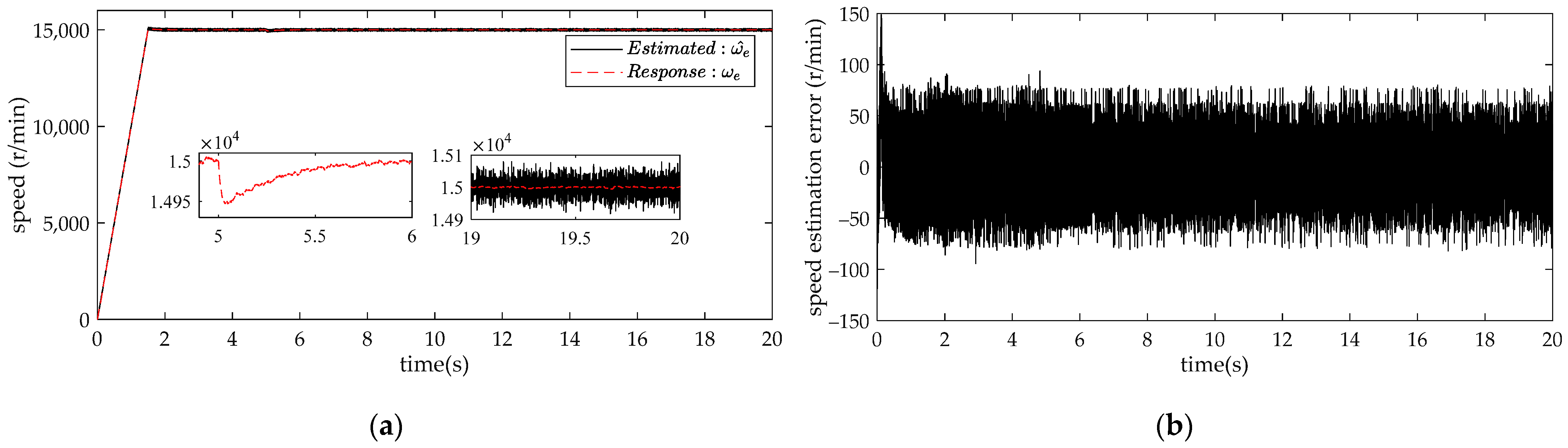
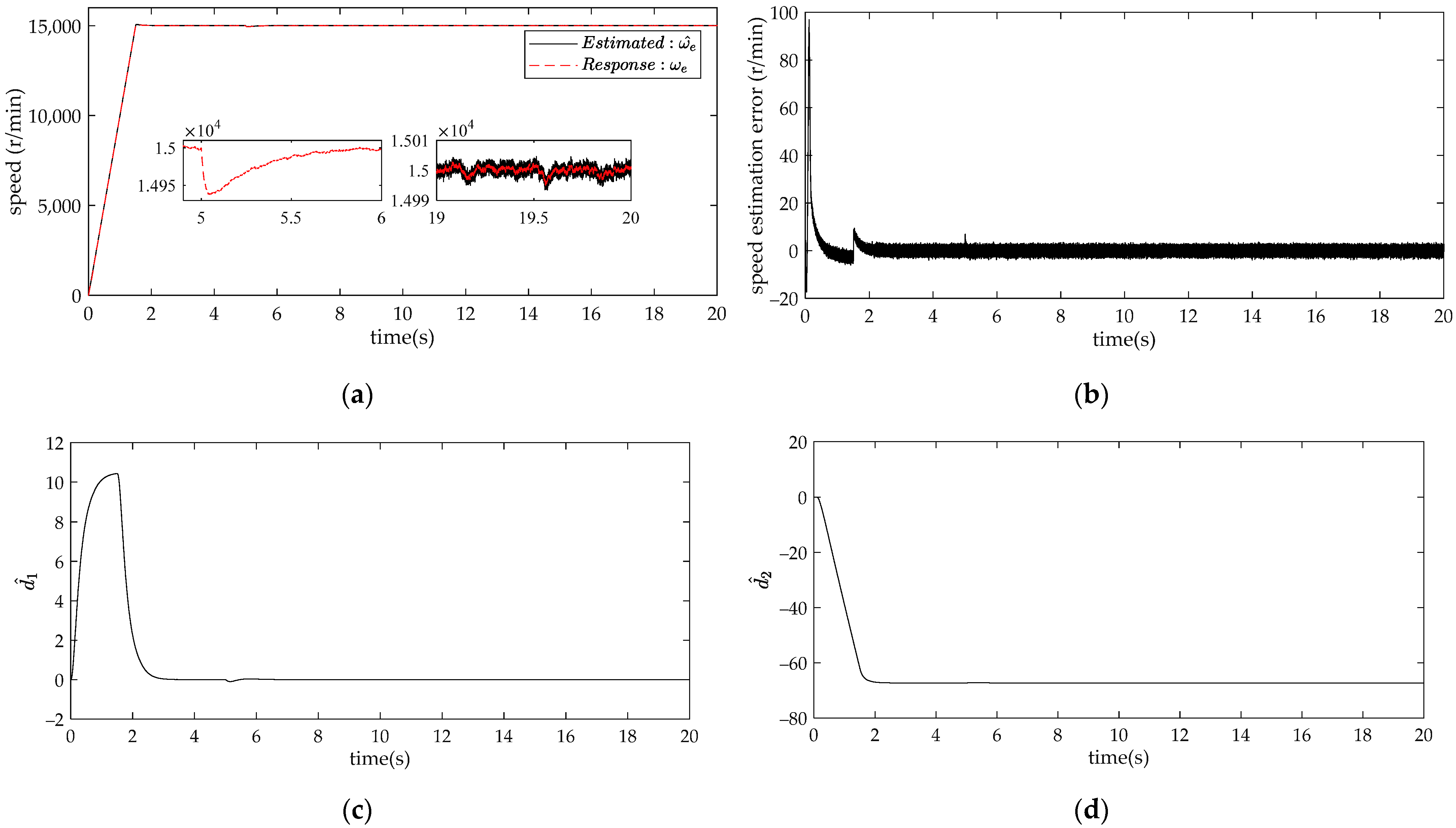
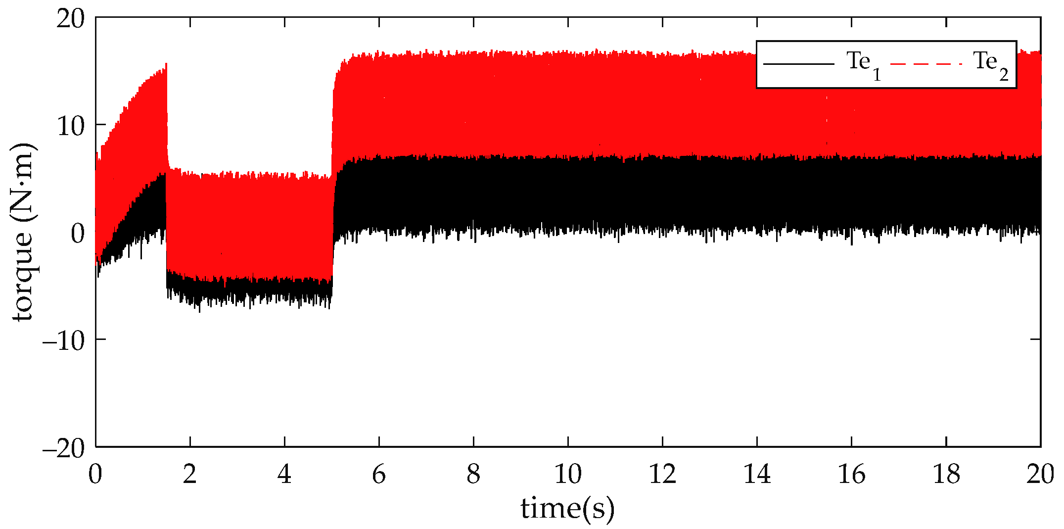
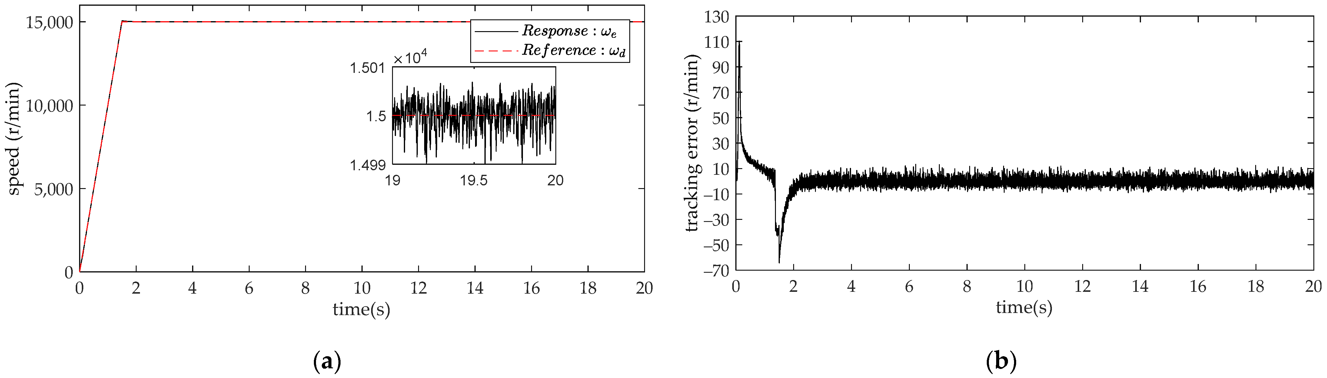
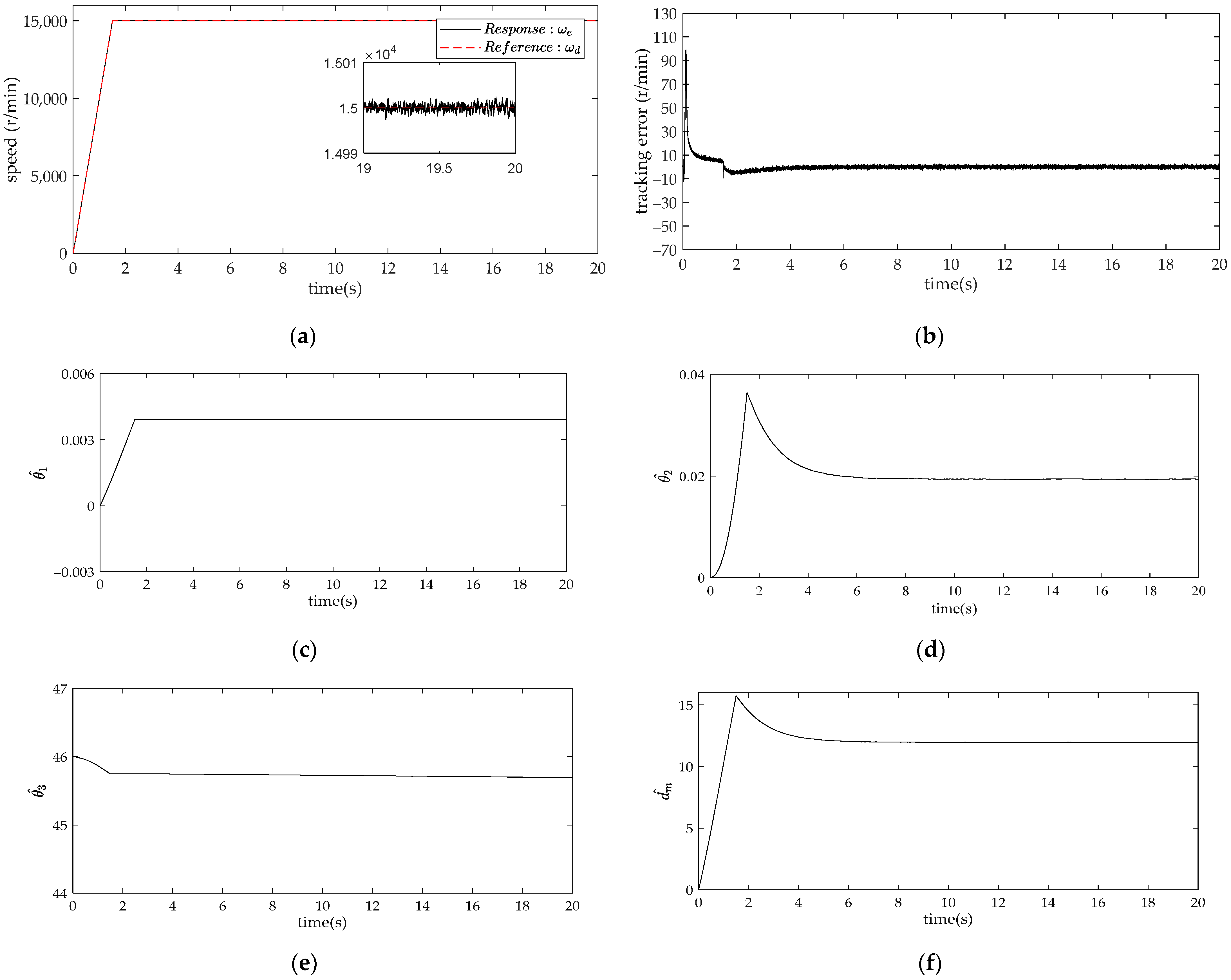
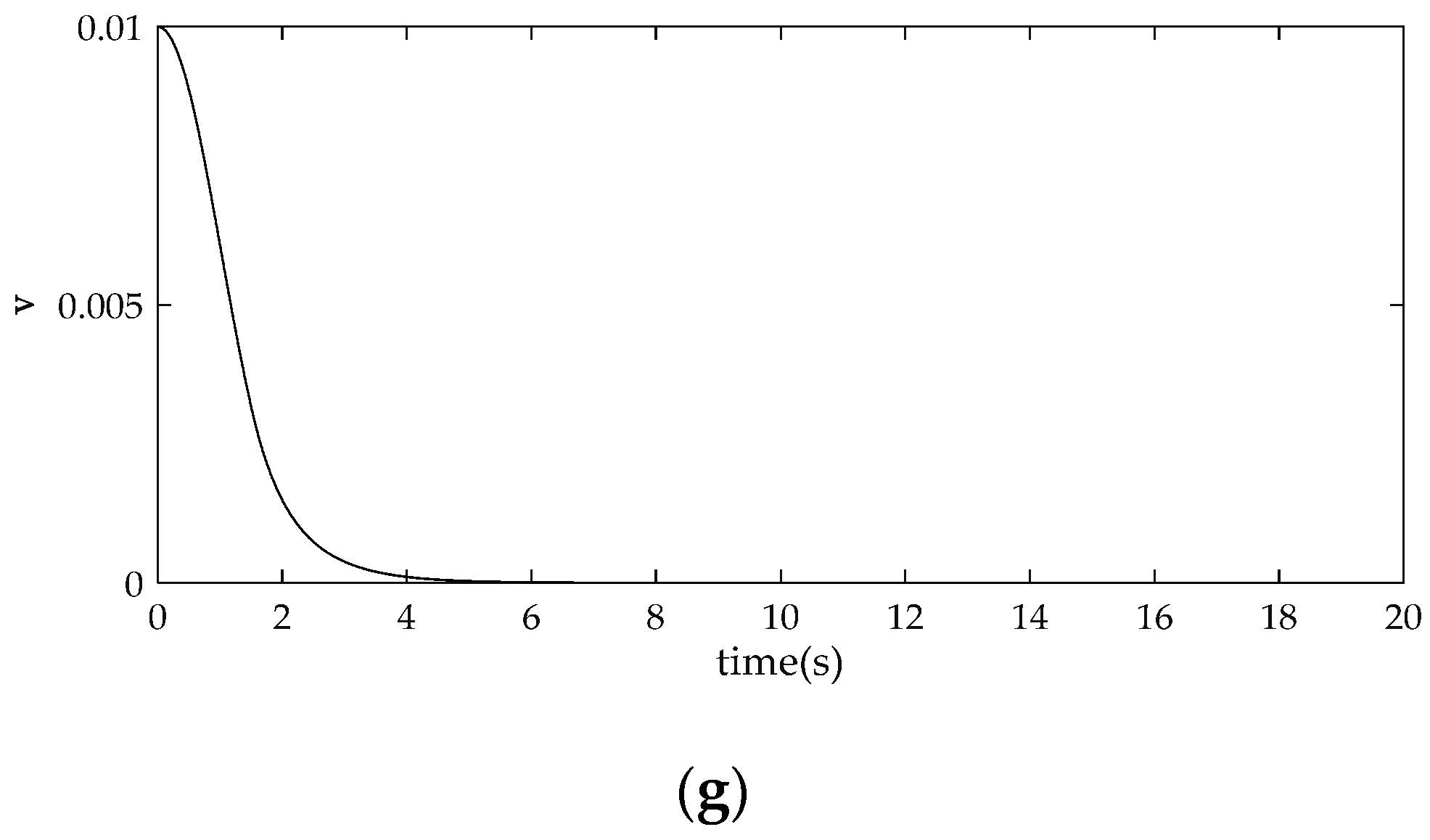
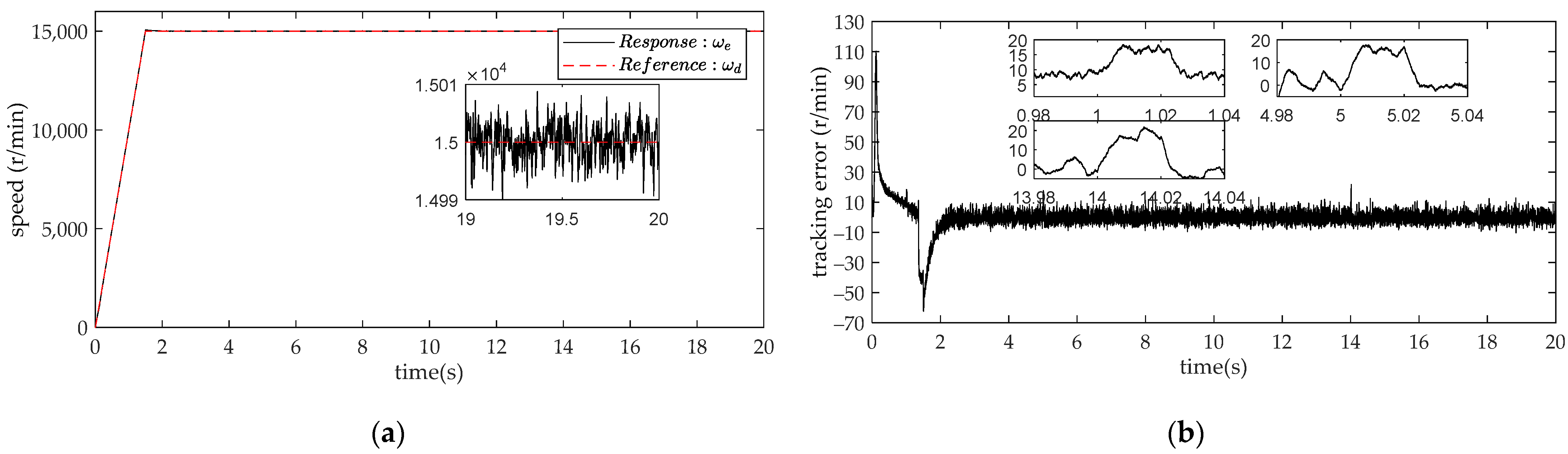
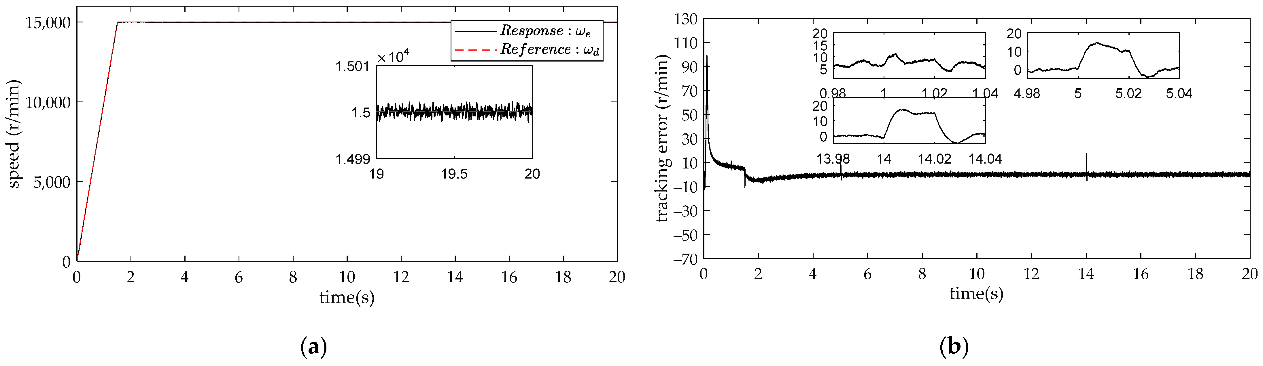
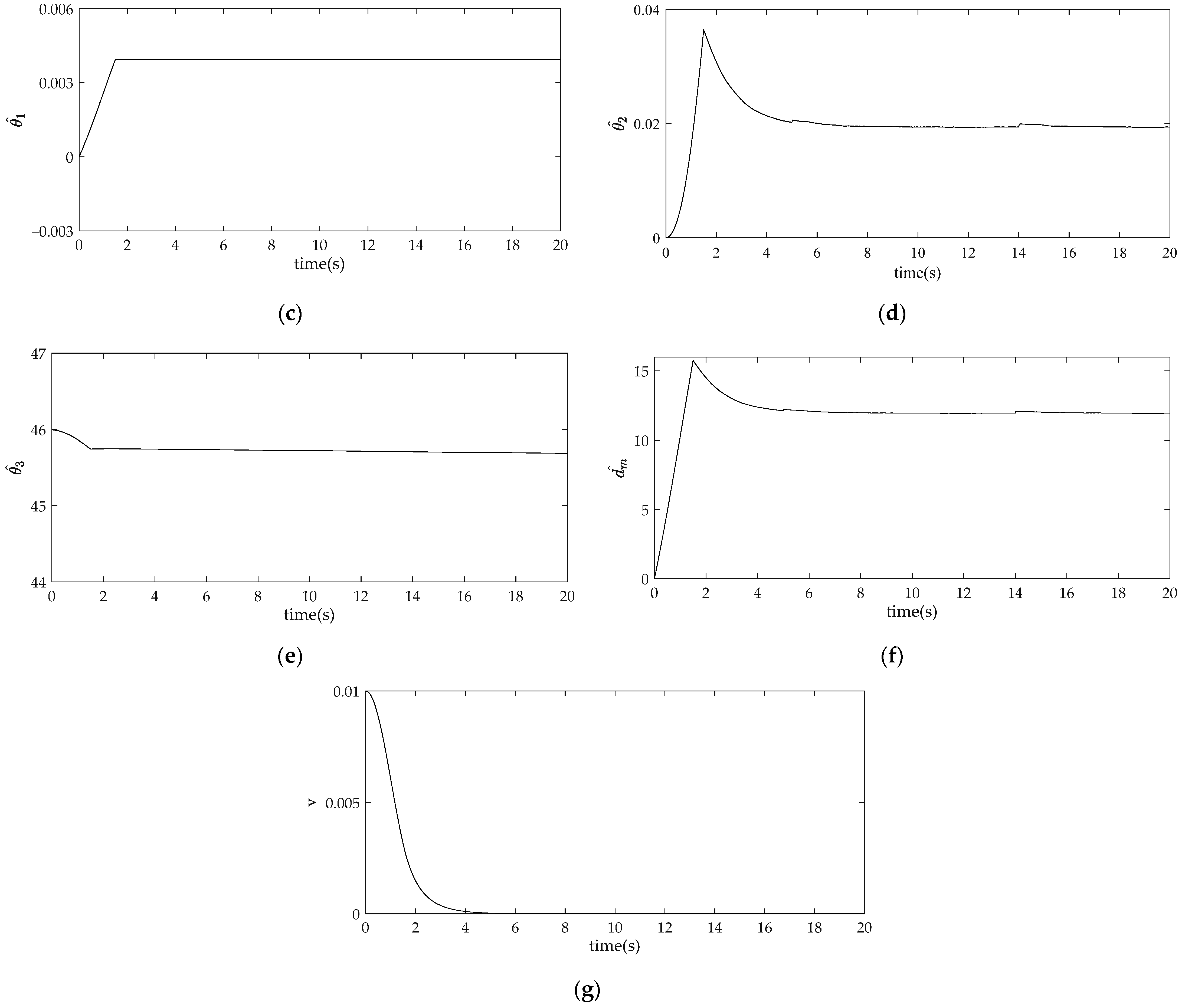
4. Comparison and Analysis of Simulation Results

The $i_{\mathrm{d}}^{*}=0$ vector control is used to simulate the control system of high-speed permanent magnet synchronous motors. Considering the influence of magnetic circuit saturation and core loss, the nonlinear relationship between the inductance, flux linkage, core loss resistance and d-q axis current is calculated by finite element analysis, and the rotor position is estimated by the sliding mode observer. This paper designs a speed controller, and the current controller uses PID control.

Figure 3 establishes the framework of a vector control system of high-speed permanent magnet synchronous motors, which consists of a high-speed permanent magnet synchronous motor (HSPMSM), space vector pulse width modulation (SVPWM) module, Park and Clark coordinate transformation, voltage source inverter, current regulator and speed controller. In addition, the stator phase resistance is 0.0244/Ω, and the no-load moment of inertia is $0.00128474/(\mathrm{kg}\cdot {\mathrm{m}}^2)$.

The design parameters of the sliding mode observer are chosen: (1) Sliding mode observer: $k_1=25$. (2) Improved sliding mode observer: $k_1=25$, $k_2=500$.

The parameters of the controller are designed as follows: (1) PID control: through the trial-and-error method, adjust the controller gain to $k_p=10$, $k_i=8$, $k_d=0$. (2) Adaptive robust control: the control strategy designed in this paper. The initial values of the unknown parameters are chosen as: $\widehat{\theta }(0)={\left[\begin{array}{ccc}0,& 0,& 46\end{array}\right]}^{\mathrm{T}}$. The parameter adaptation rates are set as ${\left[\begin{array}{ccc}{\mathsf{\Gamma }}_1& {\mathsf{\Gamma }}_2& {\mathsf{\Gamma }}_3\end{array}\right]}^{\mathrm{T}}={\left[\begin{array}{ccc}2.5\times {10}^{-6}& 3\times {10}^{-5}& 0.026\end{array}\right]}^T$ and $k_{\mathrm{e}}=500$, $k_{\mathrm{s}}=0.5$.

Using PID as the speed controller, set the given speed to 15,000 rpm and add a load of 0.5 $\mathrm{N}\cdot \mathrm{m}$ at 5 s. Figure 4 shows the performance results of the traditional sliding mode observer without considering the iron loss, and Figure 5 shows the performance results of the observer with considering the iron loss in this paper. Figure 6 shows the torque response. In Figure 6, ${\mathrm{Te}}_1$ is the torque of the traditional sliding mode observer, and ${\mathrm{Te}}_2$ is the torque of the improved sliding mode observer. From these results, it can be seen that the speed estimation effect of the improved sliding mode observer is obviously better than that of the traditional sliding mode observer. This is because a disturbance observer is added to the improved sliding mode observer, and the influence of iron loss is taken into account. The disturbance estimator is used to deal with unknown disturbances, and the parameter uncertainty is dealt with by looking up the iron loss resistance, d-q axis inductance and flux linkage in Figure 2. It is worth noting that, in 5 s, the feedback speed is affected due to the load change. However, the traditional sliding mode observer has a better anti-disturbance ability, which shows that the robustness will be sacrificed if the arctangent function is used instead of the symbolic function. It can be seen in Figure 6 that the torque of ${\mathrm{Te}}_1$ is smaller than that of ${\mathrm{Te}}_2$, because the iron core loss will reduce the actual output torque. The improved sliding mode observer can deal with the influence of iron loss and improve the performance of the system.

To verify the effectiveness of the proposed controller, the sliding mode observer is combined with the adaptive robust controller, and the speed tracking performances of the adaptive robust controller and PID controller are compared. The set speed is 15,000 revolutions, with a load of 1 N·m. The control effects of the HSPMSM system are shown in Figure 7 and Figure 8. It can be seen from the results in Figure 7 and Figure 8 that the designed adaptive robust controller is obviously superior to PID control in terms of transient and steady-state performance. The maximum control error of the adaptive robust controller is 98, and the steady-state error is less than 5.

To test the robustness of the proposed controller regarding external disturbances, we add 0.2 $\mathrm{N}\cdot \mathrm{m}$, 0.5 $\mathrm{N}\cdot \mathrm{m}$ and 0.6 $\mathrm{N}\cdot \mathrm{m}$ disturbances to the system at 1 s, 5 s and 14 s, respectively. The tracking results are shown in Figure 9 and Figure 10. It can be seen from Figure 9 and Figure 10 that the disturbance rejection effect of the adaptive robust controller based on the characteristic model is better than that of PID. Although the high-speed motor is subject to unknown disturbances, the proposed adaptive robust controller can still make the speed return to the given trajectory quickly.

5. Conclusions

In this paper, a sensorless control method has been designed. The estimation of core loss resistance and stator inductance has been used in the design of a sliding mode observer to reduce the estimation error related to parameter fluctuation. At the same time, the characteristic model has been used to design the speed controller, and the adaptive rate robust control rate has been designed to realize the accurate compensation of the system model and suppress the external interference of the high-speed motor system. Finally, the simulation results have been given to show that the proposed control method improves the accuracy of the rotor position estimation and speed tracking. In future work, we will further study the sensorless control of permanent magnet synchronous motors in the full-speed range and try to combine the low-speed operation control algorithm with the high-speed operation control algorithm.

References

1. Antivachis, M.; Niklaus, P.S.; Bortis, D.; Kolar, J.W. Input/output EMI filter design for three-phase ultra-high speed motor drive gan inverter stage. CPSSTPEA 2021, 6, 74–92. [Google Scholar] [CrossRef]
2. Kim, J.; Jeong, I.; Nam, K.; Yang, J.; Hwang, T. Sensorless Control of PMSM in a High-Speed Region Considering Iron Loss. IEEE Trans. Ind. Electron. 2015, 62, 6151–6159. [Google Scholar] [CrossRef]
3. Cao, Y.; Wang, J.; Shen, W. High-performance PMSM self-tuning speed control system with a low-order adaptive instantaneous speed estimator using a low-cost incremental encoder. AJC 2020, 23, 1870–1884. [Google Scholar] [CrossRef]
4. Ding, W.; Liang, D.L.; Luo, Z.Q. Position sensorless control of PMSM using sliding mode observer with two-stage filter. Electr. Mach. Control 2012, 11, 1–10. [Google Scholar]
5. Liu, Y.; Fang, J.; Tan, K.; Huang, B.; He, W. Sliding Mode Observer with Adaptive Parameter Estimation for Sensorless Control of IPMSM. Energies 2020, 13, 5991. [Google Scholar] [CrossRef]
6. Veluvolu, K.C.; Soh, Y.C. High-gain observers with sliding mode for state and unknown input estimations. IEEE Trans. Ind. Electron. 2009, 56, 3386–3393. [Google Scholar] [CrossRef]
7. Wu, S.; Zhang, J.; Chai, B. Adaptive super-twisting sliding mode observer based robust backstepping sensorless speed control for IPMSM. ISA Trans. 2019, 92, 155–165. [Google Scholar] [CrossRef]
8. Morimoto, S.; Kawamoto, K.; Sanada, M.; Takeda, Y. Sensorless control strategy for salient-pole PMSM based on extended EMF in rotating reference frame. Conference Record of the 2001 IEEE Industry Applications Conference. In Proceedings of the 36th IAS Annual Meeting (Cat. No.01CH37248), Chicago, IL, USA, 30 September–4 October 2001; pp. 2637–2644. [Google Scholar]
9. Xu, W.; Qu, S.; Zhao, L.; Zhang, H. An Improved Adaptive Sliding Mode Observer for Middle- and High-Speed Rotor Tracking. IEEE Trans. Power Electron. 2020, 36, 1043–1053. [Google Scholar] [CrossRef]
10. Yamamoto, S.; Hirahara, H.; Tanaka, A.; Ara, T.; Matsuse, K. Universal sensorless vector control of induction and permanent magnet synchronous motors considering equivalent iron loss resistance. In Proceedings of the Industry Applications Society Meeting, Lake Buena Vista, FL, USA, 6–11 October 2013; pp. 1–8. [Google Scholar]
11. Kumar, P.; Bhaskar, D.V.; Muduli, U.R.; Beig, A.R.; Behera, R.K. Iron-Loss Modeling With Sensorless Predictive Control of PMBLDC Motor Drive for Electric Vehicle Application. IEEE Trans. Transp. Electrif. 2020, 7, 1506–1515. [Google Scholar] [CrossRef]
12. Cui, W.; Zhang, F.-X. A Novel Sensorless Rotor Position Estimation Method for PMSM Based on High-Frequency Square-Wave Voltage Injection with Less Iron Loss. Electr. Power Components Syst. 2018, 46, 1872–1882. [Google Scholar] [CrossRef]
13. Kang, K.-L.; Kim, J.-M.; Hwang, K.-B.; Kim, K.-H. Sensorless control of PMSM in high speed range with iterative sliding mode observer. In Proceedings of the Nineteenth Annual IEEE Applied Power Electronics Conference and Exposition, 2004. APEC ‘04, Anaheim, CA, USA, 22–26 February 2004; pp. 1111–1116. [Google Scholar]
14. Zhang, X.; Liu, X.; Zhu, Q. Attitude control of rigid spacecraft with disturbance generated by time varying exosystems. Commun. Nonlinear Sci. Numer. Simul. 2014, 19, 2423–2434. [Google Scholar] [CrossRef]
15. Kayacan, E.; Fossen, T.I. Feedback Linearization Control for Systems with Mismatched Uncertainties via Disturbance Observers. Asian J. Control 2019, 21, 1064–1076. [Google Scholar] [CrossRef]
16. Mohanty, A.; Yao, B. Integrated Direct/Indirect Adaptive Robust Control of Hydraulic Manipulators With Valve Deadband. IEEE/ASME Trans. Mechatronics 2010, 16, 707–715. [Google Scholar] [CrossRef]
17. Li, Y.; Fan, Y.; Li, K.; Liu, W.; Tong, S. Adaptive Optimized Backstepping Control-Based RL Algorithm for Stochastic Nonlinear Systems With State Constraints and Its Application. IEEE Trans. Cybern. 2021, 99, 1–14. [Google Scholar] [CrossRef]
18. Cecati, C. Position Control of the Induction Motor Using a Passivity-Based Controller. IEEE TIA 2000, 36, 1277–1284. [Google Scholar] [CrossRef]
19. Yao, B.; Tomizuka, M. Adaptive robust control of SISO nonlinear systems in a semi-strict feedback form. Automatica 1997, 33, 893–900. [Google Scholar] [CrossRef]
20. Yao, B.; Bu, F.; Reedy, J.; Chiu, G.-C. Adaptive robust motion control of single-rod hydraulic actuators: Theory and experiments. IEEE/ASME Trans. Mechatron. 2000, 5, 79–91. [Google Scholar] [CrossRef]
21. Cheng, L.-J.; Tsai, M.-C. Robust Scalar Control of Synchronous Reluctance Motor With Optimal Efficiency by MTPA Control. IEEE Access 2021, 9, 32599–32612. [Google Scholar] [CrossRef]
22. Quang, L.H.; Putov, V.; Sheludko, V. Adaptive robust control of a multi-degree-of-freedom mechanical plant with resilient properties. Procedia Comput. Sci. 2021, 186, 611–619. [Google Scholar] [CrossRef]
23. Yao, J.; Jiao, Z.; Ma, D. Extended-State-Observer-Based Output Feedback Nonlinear Robust Control of Hydraulic Systems With Backstepping. IEEE Trans. Ind. Electron. 2014, 61, 6285–6293. [Google Scholar] [CrossRef]
24. Wu, H.; Hu, J.; Xie, Y. Intelligent Adaptive Control Based on Characteristic Model; China Science and Technology Press: Beijing, China, 2009; pp. 45–76. [Google Scholar]
25. Wu, H. Research and prospect on the control theory and method in the engineering. Control Theory Appl. 2014, 31, 1626–1631. [Google Scholar]
26. Wang, X.; Wu, Y.; Zhang, E.; Guo, J.; Chen, Q. Adaptive terminal sliding-mode controller based on characteristic model for gear transmission servo systems. Trans. Inst. Meas. Control 2018, 41, 219–234. [Google Scholar] [CrossRef]
27. Gao, Y.; Wu, Y.; Wang, X.; Chen, Q. Characteristic Model-based Adaptive Control with Genetic Algorithm Estimators for Four-PMSM Synchronization System. Int. J. Control Autom. Syst. 2020, 18, 1605–1616. [Google Scholar] [CrossRef]
28. Urasaki, N.; Senjyu, T.; Uezato, K. Relationship of Parallel Model and Series Model for Permanent Magnet Synchronous Motors Taking Iron Loss Into Account. IEEE Trans. Energy Convers. 2004, 19, 265–270. [Google Scholar] [CrossRef]
29. Wallsgrove, R.J.; Akella, M. Globally Stabilizing Saturated Attitude Control in the Presence of Bounded Unknown Disturbances. J. Guid. Control Dyn. 2005, 28, 957–963. [Google Scholar] [CrossRef]
Figure 1. (a) D-axis equivalent circuit; (b) Q-axis equivalent circuit.
Energies 15 07615 g001
Figure 2. (a) Variations curve of the direct axis inductance with the d-q axis current; (b) Variations curve of the quadrature axis inductance with the d-q axis current; (c) Variations curve of the flux linkage of the permanent magnet with the d-q axis current; (d) Variations curve of the iron loss equivalent resistance with the d-q axis current.
Energies 15 07615 g002
Figure 3. Overall structure block diagram of high-speed motor vector control.
Energies 15 07615 g003
Figure 4. (a) Speed estimation of the traditional sliding mode observer; (b) Estimation error.
Energies 15 07615 g004
Figure 5. (a) Speed estimation of the improved sliding mode observer; (b) Estimation error; (c) Estimated value of d 1 ; (d) Estimated value of d 2 .
Energies 15 07615 g005
Figure 6. Torque response.
Energies 15 07615 g006
Figure 7. (a) Speed response under PID control; (b) Tracking error of PID.
Energies 15 07615 g007
Figure 8. (a) Speed response under adaptive robust control; (b) Tracking error of adaptive robust control; (cg) Parameter adaptation of the proposed adaptive robust control.
Energies 15 07615 g008aEnergies 15 07615 g008b
Figure 9. (a) Speed response of PID control in case of external disturbances; (b) PID tracking error in case of external disturbances.
Energies 15 07615 g009
Figure 10. (a) Speed response of adaptive robust control in the presence of external disturbances; (b) Tracking error of adaptive robust control in the presence of external disturbances; (cg) Parameter adaptation of adaptive robust control in the presence of external disturbances.
Energies 15 07615 g010aEnergies 15 07615 g010b