Abstract
Electricity price forecasts have become a fundamental factor affecting the decision-making of all market participants. Extreme price volatility has forced market participants to hedge against volume risks and price movements. Hence, getting an accurate price forecast from a few hours to a few days ahead is very important and very challenging due to various factors. This paper proposes an integrated long-term recurrent convolutional network (ILRCN) model to predict electricity prices considering the majority of contributing attributes to the market price as input. The proposed ILRCN model combines the functionalities of a convolutional neural network and long short-term memory (LSTM) algorithm along with the proposed novel conditional error correction term. The combined ILRCN model can identify the linear and nonlinear behavior within the input data. ERCOT wholesale market price data along with load profile, temperature, and other factors for the Houston region have been used to illustrate the proposed model. The performance of the proposed ILRCN electricity price forecasting model is verified using performance/evaluation metrics like mean absolute error and accuracy. Case studies reveal that the proposed ILRCN model shows the highest accuracy and efficiency in electricity price forecasting as compared to the support vector machine (SVM) model, fully connected neural network model, LSTM model, and the traditional LRCN model without the conditional error correction stage.
1. Introduction
Wholesale energy market price, also known as settlement point prices or dynamic tariff, was discussed in the early 1980s [1]. When the electricity market is compared with other commodities, the power trade exhibits multiple attributes: constant balance between production and consumption [2]; dependence of the load with respect to time, exhibiting seasonality at the daily, weekly, and annual levels; and load and generation that are influenced by external weather conditions [3], neighboring markets [4], and other factors like fuel price [3]. In a deregulated power market such as the locational marginal pricing (LMP) based market, the prices are significantly influenced by the above-mentioned attributes.
Electricity price forecasting has become a fundamental input to market participants’ decision-making mechanisms. Generally, wholesale electricity prices are likely to be high during peak demand periods and low during off-peak demand periods [5,6]. The dynamic tariff or price is an inherent load management method for properly allocating resources, thus ensuring overall economic reliability [7]. Additionally, an electric tariff is widely utilized as a fundamental control signal to support demand response management for improving energy efficiency [8] and relieving the load burden on the power grid.
Electricity prices have a direct influence on the behavior of individual customers, distributed energy resource aggregators, and local microgrid operators that aim for maximum profit or minimum cost. Electricity prices affect their energy consumption profile and the amount of power to sell or purchase from the power grid. These characteristics lead to an abrupt change in electricity price, generally with sharp price spikes. Accurate price predictions are essential for them to make informed decisions like demand scheduling and power dispatching, which may also enhance the reliability of bulk power systems. However, it is very challenging to predict electricity prices since they are highly volatile due to unexpected peaks and troughs, continuously altering supply and demand fluctuations, various system constraints, and other factors over the course of the day. Machine learning models are able to handle such nonlinear variation with varying degrees of success. Recently, deep learning (DL) algorithms have become the state-of-art method for spatio-temporal pattern recognition in energy market prices and demand.
This paper proposes an integrated long-term recurrent convolutional network (integrated LRCN, or ILRCN) model to forecast the wholesale market electricity price. The proposed ILRCN model consists of hybrid neural network architecture, i.e., LRCN, with an additional conditional error correction layer [9]. In the case study section, the Electric Reliability Council of Texas (ERCOT) wholesale market price and its contributing factors such as load and weather conditions for the Houston region of Texas are considered to demonstrate the proposed ILRCN model. In summary, the main contributions of this paper are:
- A hybrid neural network architecture, i.e., LRCN, with an additional conditional error correction layer, is used.
- An electricity price forecasting performance analysis with both hour and day ahead comparison is made.
- The practicality and feasibility of the proposed electricity price forecasting algorithm are compared to existing algorithms.
The rest of the paper is organized as follows: Background analysis, challenges encountered in price forecasting, and current industry trends and models are covered in Section 2. Section 3 introduces the fundamentals of wholesale power energy market price and various neural networks, as well as a naive time-delayed price prediction method. Section 4 describes the proposed ILRCN model and the overall methodology. Section 5 provides the simulation results and analyzes the performance of the proposed method. Section 6 concludes the paper.
2. Literature Review
Accurate models for predicting wholesale electricity prices are necessitated due to the fact that electricity price is a fundamental input to energy companies’ decision-making mechanisms at the corporate level. A power utility company or large industrial consumer who is able to forecast the volatile wholesale prices with a reasonable level of accuracy can adjust its bidding strategy and its own production or consumption schedule in order to reduce the risk or maximize the profits in power trading. The market price depicts the substantial value of electric power.
The fluctuations in supply and demand determine the rate of change of electricity prices. Reference [10] shows how the power price variation in accordance with these fluctuations can reflect the actual value of electricity in the transaction process. Bidding procedures and settlement point price determine the profit level for participating power companies. Higher accuracy of power price prediction could enable participants to make better decisions that lead to higher profits or lower risks. There are various factors contributing to electricity price prediction: (a) quantifiable factors such as historical and recent electricity prices and loads and (b) non-quantifiable factors such as market design and network topology. All these factors greatly increase the difficulty of electricity price prediction [11].
Presently, there are various studies related to electricity price forecasting [12]. Electricity prices are utilized as a basic control signal to support demand response management, which is a feasible solution for improving energy efficiency. Price forecasting benefits the power grid as it offers specific price instructions for participants to manage their flexible power usage at different times, which alleviates the load burden of the power grid, especially in peak demand time. Additionally, price forecasting also encourages consumption by end users during periods of valley demand along with reduced prices and allows customers to have multiple choices to determine the period of peak consumption. Amjady [13] explained the need for short-term electricity price forecasting and proposed models for such predictions.
A drawback of various statistical models proposed previously in the literature like auto-regressive, dynamic regression, and transfer function is the fact that they use linear forecasters; as such, they do not perform well where the periodicity of input data is high, e.g., hourly data with rapid variations. In other words, the nonlinear behavior of hourly prices might become too complicated to predict [14]. However, these models perform adequately if the data frequency is low, e.g., weekly/monthly patterns with small variations. To address the issues in statistical models and predict the nonlinear characteristics of electricity prices, different machine learning methods have been proposed. Among them, multilayer perceptrons (MLPs), support vector regressors, and radial basis function networks are the most widely used.
Over the last decade, the field of neural networks has undergone several shifts that have led to what is today known as deep learning. The major issue of neural networks has always been the heavy computational complexity and computational cost of training large models. However, this issue can be addressed; for instance, in [15], a deep neural network was trained efficiently using an algorithm called greedy layer-wise pre-training or batch training process. As related developments followed, researchers were able to efficiently train complex neural networks whose depth was not just limited to a single hidden layer (as in the traditional multilayer perceptron).
In [16], a hybrid model with the combined kernel function was used for price forecasting of the Australian electricity market. Reference [17] used generalized mutual information for the normalization of input data and a least square support vector machine for day-ahead price forecasting. Reference [18] also employed a hybrid algorithm for load and price forecasting along with a simultaneous prediction of peak hour load and day-ahead price, applied on different datasets of NYISO and PJM accordingly. This was further being used to optimize demand side management in [19]. Deep neural network [20], gated recurrent unit [21], shallow neural network, and long short-term memory (LSTM) [22] models are efficient forecasting methods that aid in increasing their prediction accuracy compared to traditional statistical models. However, the benefits of these models are not exhibited completely due to continuous fluctuation in the market price.
Other energy related applications and use cases showed excellent results obtained in time series prediction [23,24], where electricity price prediction is possible by using DL architectures. In reviewing the above details, we focused our research on modelling the wholesale electricity price forecasting using the proposed ILRCN model which can identify the nonlinear behavior of market prices due to various uncertainty factors contributing to energy prices.
3. Preliminaries
In this section, theoretical concepts of deep learning and fundamentals of electricity price are introduced.
3.1. Electricity Market Price
There are two main types of electricity market prices: day-ahead market (DAM) price and real-time market (RTM) price [25]. In the day-ahead market, bids are submitted for interval hours of the operating day one day in advance, while real-time market bids are submitted only a couple of hours in advance. These bids are highly dependent on several factors, including the demand for the particular interval, demand response operating for the area, weather conditions, and bidding strategies for the participating players. These bids are defined per interval, i.e., every market player can submit bids or use default bids. Market operators use the collected bids to compute the market settlement point price for each interval, as well as the generation schedule.
Locational marginal pricing is used to price energy on the market in response to changes in supply and demand and the system’s physical constraints. LMP accounts for the cost to produce the energy, the cost to transmit this energy within regions of the market, and the cost due to power losses as the energy is transported across the system.
3.2. Naive Method
The naive method implemented in this paper serves as a benchmark to gauge the proposed ILRCN model as well as other price prediction models. It is a time-delayed price determination method that (i) simply takes the electricity prices of day d − 1 as the forecasted electricity prices of day d when conducting real-time price prediction one day ahead, or (ii) simply takes the electricity prices of hour t − 1 as the forecasted electricity prices of hour t when conducting real-time price prediction one hour ahead. This naive method works best for short-term price forecasting (predictions over a short look-ahead period such as 15 min), where the electricity price has relatively less volatility and is unlikely to change substantially during consecutive short time intervals.
3.3. Support Vector Machine
Support vector machine (SVM) is a supervised type of machine learning algorithm which is based on Statistical Learning Theory. Due to its greater ability to generalize the problem, SVM has been successfully applied in classification tasks and regression tasks, especially in time series prediction and financial-related application.
When using SVM in regression tasks, the Support Vector Regressor (SVR) uses a cost function to measure the empirical risk [26]. For given training data , where denotes the space of the input data. Basically, the goal of regression is to find the function that best models the training data, and at the same time as flat as possible. The case of linear function can be described as,
where denotes the dot production in . To construct the optimal hyperplane, which can be used for regression, the problem can be reformulated as a convex optimization problem:
Constraint (3) ensures the convex optimization problem is feasible. In this study, the SVR model is built based on the historic data to subsequently predict the electricity market [27]. The goal of SVR training is to minimize the sum of squares error on the training set.
3.4. Deep Neural Network
Deep learning brings about an explosion of data in all forms across the globe. The multilayer perceptron is a fully connected neural network (FCNN) architecture with one input layer, one or multiple hidden layers, and one output layer. In FCNN, all the neurons of the previous layer are fully connected to the neurons of the next layer as shown in Figure 1.
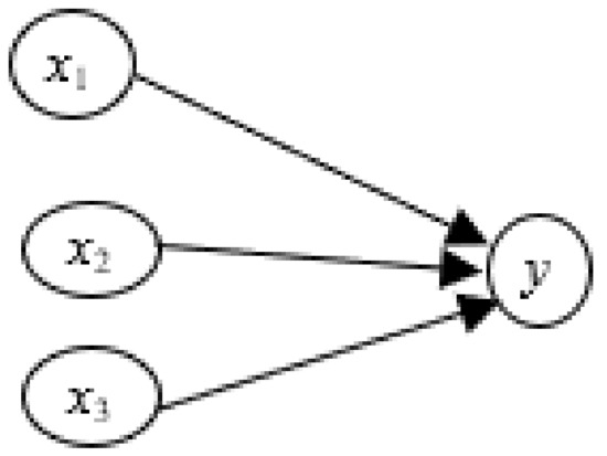
Figure 1.
A sample portion of the FCNN model.
The basic DL model, an FCNN model, is an extension of the traditional MLP that uses multiple hidden layers. Each layer consists of a defined number of neurons. In Figure 1, x1, x2, and x3 are the input neurons of the previous layer and y is the neuron of the next layer, which is the output in this scenario. The y can be calculated by the following computation equation:
where i denotes the weights of the neurons and b is the bias value; xi is the input neuron. A basic DL model would require an activation function to be trained efficiently where each neuron is activated in each layer after the computation of y in the preceding layer.
3.5. Convolutional Neural Network
The convolutional neural network (CNN) [28,29,30] utilizes the concept of weight sharing, which provides better accuracy in highly nonlinear problems such as power price forecasting. It’s an expansion from a basic deep learning model. An example of a convolutional neural network is shown in Figure 2 [31].
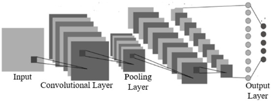
Figure 2.
Convolutional neural network architecture [31].
CNN consists of different types of hidden layers:
- (1)
- Convolutional Layer: The convolutional layer operates on two signals—(a) input and (b) filter (kernel) on the input. The underlying process here is the matrix multiplication of the input set and kernel to get the modified input, which extracts the information from the entire input using the kernel to obtain the essential data.
- (2)
- Pooling Layer: It is a sample-based discretization process. It aims at reducing the dimensionality of an input feature (e.g., input data, feature extraction) and extracting the information about the relation between input and output contained in the subset.
- (3)
- Output Layer: It is also known as the fully connected layer that connects every neuron in one layer to every neuron in the subsequent layer.
3.6. Long Short-Term Memory Neural Network
Recurrent neural network (RNN) is another framework of DL, which uses the internal state to process a sequence of inputs [32]. Long short-term memory is an extended framework of RNN which can exhibit the temporal behavior of time series input data. LSTM is capable of learning long-term dependencies from time sequential data such as electricity prices. The fundamental equations of an LSTM network can be represented as follows:
where, xt is the network input; ht is the output state of the neuron from the LSTM network; ht−1 is the previous state of the neuron; zt computes the necessary information and removes the irrelevant data; is the sigmoid function; Wf is the weight function; and bf is the bias value.
3.7. Nonlinearities in Electricity Prices
LMP is the basis of wholesale power market mechanisms for many nations, including the United States. LMP is affected by a number of influencing factors including demand, available supply, network topology and losses, system constraints, and climatic conditions. The congestion component of LMP accounts for the network constraints that bind the optimal generating strategy. Overall, LMP could vary substantially for different locations and time intervals and it is highly nonlinear.
Figure 3, Figure 4 and Figure 5 show the variation of ERCOT prices with respect to different time horizons. Figure 3 displays the RTM settlement price variation over the course of a day, showing the non-linear and continuous fluctuation of electricity prices. According to Figure 4 and Figure 5, it is evident that the price dynamics have various seasonal patterns, corresponding to a daily and weekly periodicity, and are also influenced by a calendar effect, i.e., weekdays versus weekends and holidays. These properties also apply to the demand. The essential component for accurate price prediction is understanding the variation of price, i.e., identifying peaks and troughs and their relation to the governing factors contributing to changes in price.
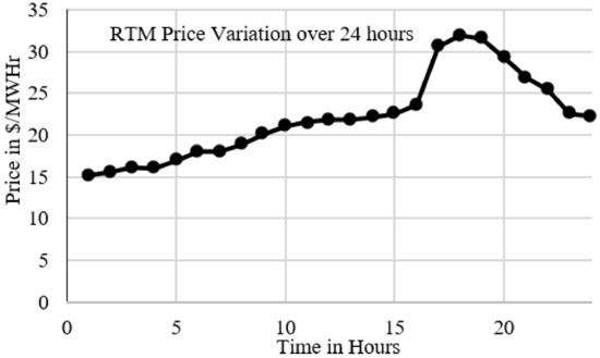
Figure 3.
Variation of settlement point price with respect to time in hours.
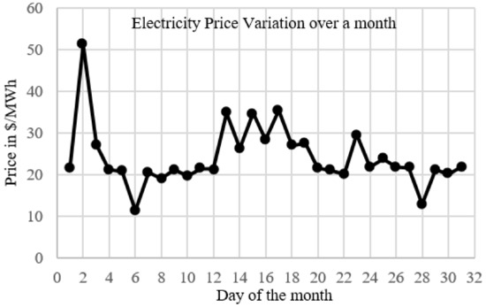
Figure 4.
Variation of settlement point price over a month.
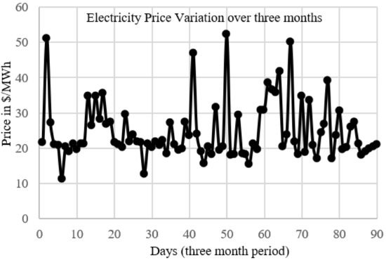
Figure 5.
Variation of settlement point price over three months.
4. System Model
The price forecasting is classified into short-term, medium-term, and long-term forecasting [33]. A short term ranges from one hour ahead to several hours ahead; a few hours to 1 week ahead forecasting is medium-term forecasting; and beyond that it is long-term forecasting. We focus on hour-ahead and day-ahead forecasting in this work. The proposed forecasting model can be formulated as:
where t is the current time interval; MPt is the forecasted market price by the proposed ILRCN model; Ft is the price forecasted by the hybrid neural network model, LRCN, that is explained in Section 4.2; and is the electricity price forecasting error correction component from the previous time interval and is also referred to as the calibrated value that is defined in Section 4.3.
The aims to reduce forecasting errors that are partially due to insufficient details/features contributing to energy price in the dataset under consideration. It can consider the prediction errors of a few previous time intervals.
Figure 6 illustrates the flowchart of short-term electricity price forecasting using the proposed ILRCN model based on several prior hours of input data. The historical data is the input forming the initial stage for the establishment of the proposed ILRCN model. The linear and nonlinear behavior and characteristics of the input data are analyzed using the proposed ILRCN model. Input feature pre-processing is used to normalize, scale, and define the features from the input data to improve the accuracy of price forecasting. In order to tune the parameters of the model, optimization and hyper-parameter tuning method with cross-validation are utilized along with the LRCN model. Finally, the forecasted price coming from the proposed LRCN model is adjusted to incorporate the conditional error correction component; the desired output is then obtained in this study.
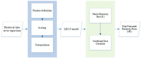
Figure 6.
Flowchart of short-term electricity price forecasting with ILRCN.
The detailed explanation of the various components of the proposed ILRCN model is introduced in detail in the following subsections.
4.1. Feature Definition and Preprocessing
Electricity prices are mainly affected by electrical demand, which varies over time depending on the season, weather, and generation cost [34]. In order to forecast the market electricity price, the date of delivery, temperature, and load data are selected as input features. The input data are normalized using various scaling functions to avoid excess stress on a specific dimension during the training process. For the date of delivery data which has no ordinal relationship, one-hot encoding is applied, and a min-max scalar technique is used to bound the temperature values within [0, 1]. After the normalization process, all major features contributing evidently to the electricity price are selected and defined to avoid over-fitting during the training process. After the feature selection process, the processed data are converted into a moving windowed dataset, where preceding interval data and features are the inputs to forecast the current output, which is the electricity price of the current interval.
4.2. Long-term Recurrent Convolutional Network
The artificial neural network is a nonlinear model capable of making accurate predictions for forecasting problems mentioned in [3]. The main parameters of the neural network model are the number of input vectors, the number of layers, and the number of neurons in each layer [15,16,19]. However, the large and sudden spikes in the input data evident from Figure 3, Figure 4 and Figure 5 will lead to less accuracy in the output. To mitigate the impact of the price outliers, an error correction stage is considered in this study; the proposed conditional error correction term can partially account for the unavailability of information in the input dataset under consideration contributing to any sudden variation in price.
Based on (4) to (6), the neural network model is employed to capture the relationship and the linear and nonlinear behavior within the input data. After the input processing stage, the processed data and the best subset of parameters containing the information obtained from input features are used in the proposed ILRCN model to forecast electricity prices.
Figure 7 shows the structure of the proposed LRCN model, a hybrid neural network, which corresponds to the third block in Figure 6. The proposed LRCN model includes two 1D convolution layers in the CNN segment, which aim to process spatial features and improve training efficiency. Two LSTM layers are added after the second convolution layer in the model to capture the dependencies in the sequential data. LSTM shows improved performance in time-series data when compared to traditional models such as a statistical forecasting model and regression model. In general, rectified linear unit (ReLU) is a widely used activation function as described in (8).
where is the input features mapped as neuron.
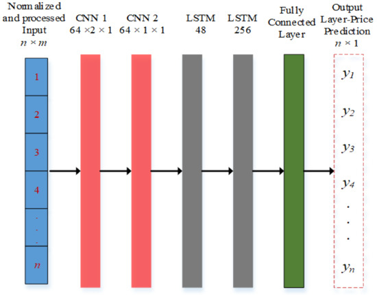
Figure 7.
The architecture of the proposed LRCN model.
This hybrid neural network can be used to build a function to express variation amongst historical data. Assuming the first input data H of the total input data set consist of n preceding hours’ wholesale electricity price data, H can then be formulated as:
where represents the input data that are the ith interval prior to the currently being predicted interval, and i ranges from 1 to n.
Henceforth, D can be expressed as:
where represents the features of the input set such as temperature, load, and date.
4.3. Conditional Error Correction Term
It is unlikely that the LRCN model can predict the outlier prices with high accuracy. The forecasting error can be substantial when there are great differences among the input data sets due to nonlinearities and spikes in the input data and when there is not sufficient information available for accurate prediction. To address this issue, we propose a novel conditional error correction term that is added to the price forecasted by the LRCN model to establish the price prediction.
The predicted value of the electricity price from the model is compared with the actual value of the settlement point price obtained from ERCOT. Then, the calibrated value from (7) accounting for insufficient input features contributing to electricity price is formulated as follows:
where denotes the actual price of time interval t − 1; Ft−1 is the forecasted price of the same time interval t − 1 by the proposed ILRCN model.
Since the LRCN model can handle regular electricity prices well, the proposed conditional error correction term will only be applied in scenarios wherein the electricity price is very high and the error of price forecasting in the previous time period is beyond the pre-specified threshold.
4.4. Metrics
The accuracy percentage of price forecasting models is defined in (12). It is very unlikely to predict the exact price; as a result, the number of correctly predicted prices in (12) is counted with an error threshold that is the maximum acceptable deviation of the predicted price from its actual value. The error threshold ranges from 1 $/MWh to 3 $/MWh in this paper.
The mean absolute error (MAE) represents the average of the absolute difference between the actual and predicted values in the dataset. The mean absolute error for the training process is calculated as follows:
where N represents the number of data points; is the actual value of electricity price of the training data point indexed by ; and is the predicted value of electricity price of the same training data. Note that this metric MAE can also be used on the validation dataset.
The mean squared error (MSE) measures the average squared difference between actual and predicted outputs. The goal of training is to minimize MSE via back propagation that provides the best estimator. The MSE is defined as:
5. Simulation Results
The proposed forecast model is tested against the Texas electricity market, ERCOT, to validate its effectiveness and efficiency. This paper employs the hourly settlement point hub price series of the Houston region of ERCOT as a test example of our model [25].
The ERCOT electricity market covers most of the state of Texas, with four regional market zones comprised of the coast (Houston), west, north, and south of Texas as sub-regions. Bids are submitted by participating companies on an interval basis. ERCOT then optimally schedules the generating units based on economics and reliability to meet the system demand while observing resource and transmission constraints; it determines the locational marginal price, which is the wholesale electricity price.
The electricity price data originally collected from ERCOT are its real-time market data that are settled down with 15-min time intervals. In this study, hourly resolution is used. The electricity price per hour is calculated by averaging the prices over four consecutive 15-min dispatches in the same hour. The COAST (Houston) region in ERCOT electricity market is employed in the study. The electric energy price, demand data, and temperature data covering the period from January 2015 to December 2018 are collected for testing.
In this study, a total of 34,542 samples were collected, and the entire dataset is first divided into two subsets: 31,087 samples (90%) for training and 3455 samples (10%) for validation. The initial learning rate was set as 0.01, and a learning rate schedule was applied in the training process by reducing the learning rate accordingly. The factor by which the learning rate was reduced was set as 0.1, and the patience value was set 50 epochs. To leverage the fast-computing abilities of Keras, the machine learning model was trained on NVIDIA RTX 2070 GPU (NVIDIA, Santa Clara, CA, USA).
Figure 8 shows the MSE of the training and validation data sets. It can be observed that the MSE decreased with the increase in the number of epochs. It should be noticed that the MSE stopped decreasing at around epoch 200, and hence the training was stopped to obtain the best model.
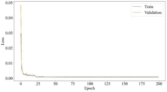
Figure 8.
MSE loss of the proposed ILRCN model with the number of epochs.
The prediction accuracies for the proposed ILRCN model and other benchmarking models are constructed for different error thresholds. Table 1 shows the accuracy percentages for hour-ahead and day-ahead forecasting using the naive method explained in Section 3 for the test dataset. With a tolerance of 3 $/MWh, the hour-ahead forecasting had a validation accuracy of 71.55% while the day-ahead forecasting achieved a much lower accuracy of 46.61%, which implies that the hour-ahead forecasting outperforms the day-ahead forecasting by a large margin. This is as expected since the naive method simply uses the current price as the future price and works fine only for predictions over very short look-ahead periods.

Table 1.
Accuracy percentages using naive method for hour-ahead forecasting and day-ahead forecasting.
Table 2 compares the results of an SVR model, an FCNN model, an LSTM-only model, the proposed LRCN model without the proposed conditional error correction term, and the proposed ILRCN model with conditional error correction for the same selected test data for hour-ahead forecasting. It is worth noting that the proposed ILRCN model had the highest validation accuracy of 85.55% with a tolerance of 3$/MWh after training of 200 epochs.
Table 2.
Accuracy percentage comparison between FCNN model, LSTM model, LRCN model, and the proposed ILRCN model for hour-ahead forecasting.
Table 3 compares the results of an SVR model, an FCNN model, an LSTM-only model, and the proposed LRCN and ILRCN models for the same selected test data for day-ahead forecasting. The LRCN model had very similar validation accuracy to the LSTM model, while the proposed ILRCN model had an accuracy of 74.41%, which outperformed all other models.
Table 3.
Accuracy percentage comparison between FCNN model, LSTM model, LRCN model, and the proposed ILRCN model for day-ahead forecasting.
Comparing Table 2 and Table 3, it is observed that the SVR model provided the same results when it predicted a day ahead or an hour ahead; this is because the SVR model does not capture the time series information and considers all samples independently. This is similar for FCNN, because FCNN can improve its prediction accuracy slightly by retraining it with additional information of the operating day.
From Table 1 and Table 3, we can observe that for both hour-ahead and day-ahead forecasting of wholesale electricity price, the proposed ILRCN model outperformed the SVR model, FCNN model, LSTM model, and LRCN model by a large margin, as well as the naive method explained in Section 3. This demonstrates the efficacy of the proposed ILRCN model for hour-ahead and day-ahead electricity price prediction. It is interesting to observe that the SVR and FCNN models could not match the naive method while all other neural network based models performed much better than the naive method in both hour-ahead prediction and day-ahead prediction.
The effectiveness of the proposed conditional error correction term can be demonstrated by comparing the performances of the proposed LRCN model and the proposed ILRCN model. When using a threshold of $3/MWh, the proposed ILRCN model slightly outperformed the LRCN model by 1.15% for hour-ahead prediction or by 3.05% for day-ahead prediction. However, when applying a threshold of $1/MWh, the proposed ILRCN model could achieve much better accuracy by a large margin of 5.78% for day-ahead prediction or 6.16% for hour-ahead prediction.
The performance metrics, like absolute error of the forecasting results, mean absolute error for the training process, and total training time, are also computed for various forecasting models and the results are presented in Table 4 and Table 5. It can be observed that the MAE and MSE of the proposed ILRCN model were 0.0254 and 0.0015 respectively for hour-ahead forecasting, which was the lowest among all models. Though it has been demonstrated that the training time for the proposed ILRCN model is comparatively more for the hour-ahead case, the prediction accuracy percentage was higher and absolute error was considerably lower, which indicates the effectiveness of the proposed ILRCN model. It is interesting to note that for day-ahead forecasting with the LRCN and ILRCN models, with the CNN layer included, the computation time for training was reduced considerably while the accuracy increased slightly when compared to the LTSM model, which proves the efficiency of the proposed LRCN architecture. The training time for the LRCN model and ILRCN model was the same because the conditional error correction term included in the proposed ILRCN model is only used in prediction (not used in training) to mitigate the imperfectness of the trained LRCN model.
Table 4.
Performance metrics of different models for hour-ahead forecasting.
Table 5.
Performance metrics of different models for day-ahead forecasting.
Figure 9 shows the comparison between the predicted settlement point price by the LRCN model and the actual price for a subset of the test data under consideration. It is evident from Figure 9 that the LRCN model does not completely track the variation in settlement point price especially for price spikes. The hour-ahead forecasted settlement point prices by the proposed ILRCN model and the actual prices are shown in Figure 10; it can be observed that the proposed ILRCN model can very well track the price variation and even the price spikes.
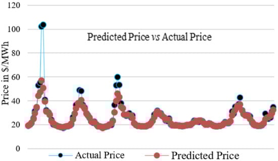
Figure 9.
Hour-ahead forecasted settlement point price by the LRCN model vs. the actual price.
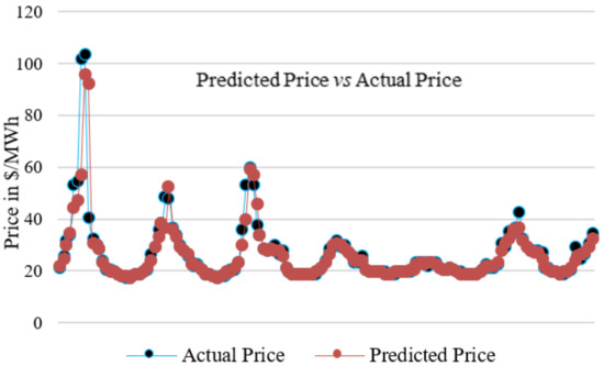
Figure 10.
Hour-ahead forecasted settlement point price by the proposed ILRCN model vs. the actual price.
To summarize, the proposed ILRCN model can achieve the highest accuracy and lowest error in real-time wholesale power energy market electricity price prediction than all other models studied in this paper, including a naive method, an SVR model, an FCNN model, an LSTM model, and an LRCN model. Although the LSTM model can also obtain a decent accuracy, its training time is about 7 times longer than the LRCN and ILRCN models, which demonstrates the efficiency of the architecture of the proposed LRCN model. Note that the above results are achieved only with the use of demand, date, and temperature information as input features. Moreover, the electricity price we predict is the real-time market price, which is much more volatile than the day-ahead market price; persistent volatility consequently results in reduced accuracy for electricity price forecasting. This implies that the proposed ILRCN model may achieve even better results when predicting the electricity price of the day-ahead market.
6. Conclusions
This paper proposes an ILRCN model to predict wholesale market electricity prices. Various dominant factors like demand profile and temperature are considered as input features for electricity price forecasting. The proposed ILRCN model for wholesale market electricity price forecasting outperforms the SVR model, FCNN model, LSTM model, and the LRCN model, as well as the naive method in terms of various metrics including training efficiency, accuracy, MSE, and MAE, as demonstrated in the case studies section.
The proposed ILRCN model predicts the electricity price with high accuracy and low error both hour-ahead and day-ahead as compared to the naive method, SVR, FCNN, LSTM, and LRCN models. The proposed conditional error correction term can further improve the prediction performance of the ILRCN model. In summary, the proposed ILRCN model outperforms both the traditional models and other neural network models, and it is proven to be an accurate and efficient model in settlement point price forecasting. The practicality and feasibility of the proposed ILRCN model are confirmed by the performance metrics. Accurate price prediction also benefits utility companies when formulating their long-term strategies. With minor adjustments and tuning, the ILRCN model proposed in this paper may also be applied in other fields such as load forecasting and variable renewable generation forecasting.
Due to limited data access, the input dataset does not contain any details on generation capacity, electrical network, bidding information, and availability of distributed energy resources in the network that also contribute to settlement point price. For future research, more information from the generator and utility side can be incorporated into the algorithm and further improve the performance of the model with better electricity price movement tracking capability.
Author Contributions
Data curation, V.S.; Formal analysis, V.S. and M.T.; Investigation, V.S. and M.T.; Methodology, V.S., M.T. and X.L.; Resources, X.L.; Supervision, X.L.; Writing–original draft, V.S. and M.T.; Writing–review & editing, M.T. and X.L., V.S. and M.T. contributed to this work equally. All authors have read and agreed to the published version of the manuscript.
Funding
This research received no external funding.
Data Availability Statement
Relevant data and codes for this research are available at: https://github.com/rpglab/WholesaleElectrPricePredict.
Conflicts of Interest
The authors state that there is no conflict of interest.
References
- Garcia, E.V.; Runnels, J.E. The utility perspective of spot pricing. IEEE Trans. Power Appar. Syst. 1985, 6, 1391–1393. [Google Scholar] [CrossRef]
- Shahidehpour, M.; Yamin, H.; Li, Z. Market Overview in Electric Power Systems. Market Operations in Electric Power Systems; John Wiley & Sons, Inc.: New York, NY, USA, 2002; Chapter 1; pp. 1–20. [Google Scholar]
- Wer Weron, R. Electricity price forecasting: A review of the state-of-the-art with a look into the future. Int. J. Forecast. 2014, 30, 1030–1081. [Google Scholar] [CrossRef]
- Lago, J.; De Ridder, F.; Vrancx, P.; De Schutter, B. Forecasting day-ahead electricity prices in Europe: The importance of considering market integration. Appl. Energy 2018, 211, 890–903. [Google Scholar] [CrossRef]
- Yu, R.; Yang, W.; Rahardja, S. A statistical demand-price model with its application in optimal real-time price. IEEE Trans. Smart Grid. 2012, 3, 1734–1742. [Google Scholar] [CrossRef]
- Luo, X.; Zhu, X.; Lim, E.G. Load scheduling based on an advanced real-time price forecasting model. In Proceedings of the 2015 IEEE International Conference on Computer and Information Technology; Ubiquitous Computing and Communications; Dependable, Autonomic and Secure Computing; Pervasive Intelligence and Computing (CIT/IUCC/DASC/PICOM), Liverpool, UK, 26–28 October 2015; pp. 1252–1257. [Google Scholar]
- Chang, C.S.; Yi, M. Real-time pricing related short-term load forecasting. In Proceedings of the 1998 International Conference on Energy Management and Power Delivery, Singapore, 5 March 1998; pp. 411–416. [Google Scholar]
- Qian, K.; Zhou, C.; Allan, M.; Yuan, Y. Modeling of load demand due to battery charging in distribution systems. IEEE Trans. Power Syst. 2011, 26, 802–810. [Google Scholar] [CrossRef]
- Donahue, J.; Hendricks, L.A.; Rohrbach, M.; Venugopalan, S.; Guadarrama, S.; Saenko, K.; Darrell, T. Long-term Recurrent Convolutional Networks for Visual Recognition and Description. IEEE Trans. Pattern Anal. Mach. Intell. 2017, 39, 677–691. [Google Scholar] [CrossRef]
- Feijooa, F.; Silva, W.; Das, T.K. A computationally efficient electricity price forecasting model for real time energy markets. Energy Convers. Manag. 2016, 113, 27–35. [Google Scholar] [CrossRef]
- Kuo, P.H.; Huang, C.J. An electricity price forecasting model by hybrid structured deep neural networks. Sustainability 2018, 10, 1280. [Google Scholar] [CrossRef]
- Nowotarski, J.; Weron, R. Recent advances in electricity price forecasting: A review of probabilistic forecasting. Renew. Sustain. Energy Rev. 2018, 81, 1548–1568. [Google Scholar] [CrossRef]
- Amjady, N.; Hemmati, M. Energy price forecasting—Problems and proposals for such predictions. IEEE Power Energy Mag. 2006, 4, 209. [Google Scholar] [CrossRef]
- McMenamin, J.S.; Monforte, F.A.; Fordham, C.; Fox, E.; Sebold, F.D.; Quan, M. Statistical Approaches to Electricity Price Forecasting. In Pricing in Competitive Electricity Markets; Springer: Boston, MA, USA, 2000; pp. 249–263. [Google Scholar]
- Hinton, G.E.; Osindero, S.; Teh, Y.-W. A fast learning algorithm for deep belief nets. Neural Comput. 2006, 18, 1527–1554. [Google Scholar] [CrossRef] [PubMed]
- Chen, Y.; Li, M.; Yang, Y.; Li, C.; Li, Y.; Li, L. A hybrid model for electricity price forecasting based on least square support vector machines with combined kernel. J. Renew. Sustain. Energy 2018, 10, 055502. [Google Scholar] [CrossRef]
- Rodríguez, C.P.; Anders, G.J. Energy price forecasting in the Ontario competitive power system market. IEEE Trans Power Syst. 2004, 19, 366–374. [Google Scholar] [CrossRef]
- Shayeghi, H.; Ghasemi, A.; Moradzadeh, M.; Nooshyar, M. Day-ahead electricity price forecasting using WPT, GMI and modified LSSVM-based S-OLABC algorithm. Soft Comput. 2017, 21, 525–541. [Google Scholar] [CrossRef]
- Ghasemi, A.; Shayeghi, H.; Moradzadeh, M.; Nooshyar, M. A novel hybrid algorithm for electricity price and load forecasting in smart grids with demand-side management. Appl. Energy 2016, 177, 40–59. [Google Scholar] [CrossRef]
- Wang, F.; Li, K.; Zhou, L.; Ren, H.; Contreras, J.; Shafie-Khah, M.; Catalão, J.P. Daily pattern prediction-based classification modelling approach for day-ahead electricity price forecasting. Int. J. Electr. Power Energy Syst. 2019, 105, 529–540. [Google Scholar] [CrossRef]
- Wang, K.; Xu, C.; Zhang, Y.; Guo, S.; Zomaya, A. Robust big data analytics for electricity price forecasting in the smart grid. IEEE Trans. Big Data 2017, 5, 34–45. [Google Scholar] [CrossRef]
- Ahmad, A.; Javaid, N.; Guizani, M.; Alrajeh, N.; Khan, Z.A. An accurate and fast converging short-term load forecasting model for industrial applications in a smart grid. IEEE Trans. Ind. Inf. 2017, 13, 2587–2596. [Google Scholar] [CrossRef]
- Feng, C.; Cui, M.; Hodge, B.-M.; Zhang, J. A data-driven multi-model methodology with deep feature selection for short-term wind forecasting. Appl. Energy 2017, 190, 1245–1257. [Google Scholar] [CrossRef]
- Wang, H.Z.; Wang, G.B.; Li, G.Q.; Peng, J.C.; Liu, Y.T. Deep belief network based deterministic and probabilistic wind speed forecasting approach. Appl. Energy 2016, 182, 80–93. [Google Scholar] [CrossRef]
- Electric Reliability Council of Texas (ERCOT). Market Prices. Available online: http://www.ercot.com/mktinfo/prices (accessed on 1 October 2022).
- Yang, H.; Chan, L.; King, I. Support Vector Machine Regression for Volatile Stock Market Prediction; Lecture Notes in Computer Science; Springer: Berlin/Heidelberg, Germany, 2002; Volume 2412, p. 391. [Google Scholar]
- Electric Reliability Council of Texas (ERCOT). Historical DAM Load Zone and Hub Prices. Available online: https://www.ercot.com/mp/data-products/data-product-details?id=NP4-180-ER (accessed on 1 October 2022).
- Krizhevsky, A.; Sutskever, I.; Hinton, G.E. ImageNet Classification with Deep Convolutional Neural Networks. Commun. ACM 2017, 60, 84–90. [Google Scholar] [CrossRef]
- Qiu, Z.; Chen, J.; Zhao, Y.; Zhu, S.; He, Y.; Zhang, C. Variety Identification of Single Rice Seed Using Hyperspectral Imaging Combined with Convolutional Neural Network. Appl. Sci. 2018, 8, 212. [Google Scholar] [CrossRef]
- Nam, S.; Park, H.; Seo, C.; Choi, D. Forged Signature Distinction Using Convolutional Neural Network for Feature Extraction. Appl. Sci. 2018, 8, 153. [Google Scholar] [CrossRef]
- Albeiwi, S.; Mahmood, A. A Framework for Designing the Architectures of Deep Convolutional Neural Networks. Entropy 2017, 19, 242. [Google Scholar] [CrossRef]
- Murugan, P. Learning the sequential temporal information with recurrent neural networks. arXiv 2018, arXiv:1807.02857. [Google Scholar]
- Nair, K.R.; Vanitha, V.; Jisma, M. Forecasting of wind speed using ann, arima and hybrid models. In Proceedings of the 2017 International Conference on Intelligent Computing, Instrumentation and Control Technologies (ICICICT), Kerala, India, 6–7 July 2017; p. 170. [Google Scholar]
- Banadaki, A.D.; Feliachi, A. Big Data Analytics in a Day-Ahead Electricity Price Forecasting Using Tensor Flow in Restructured Power Systems. In Proceedings of the 2018 International Conference on Computational Science and Computational Intelligence (CSCI), Las Vegas, NV, USA, 12–14 December 2018; pp. 1065–1069. [Google Scholar]


Publisher’s Note: MDPI stays neutral with regard to jurisdictional claims in published maps and institutional affiliations. |
© 2022 by the authors. Licensee MDPI, Basel, Switzerland. This article is an open access article distributed under the terms and conditions of the Creative Commons Attribution (CC BY) license (https://creativecommons.org/licenses/by/4.0/).