
3D Geomechanical Model Construction for Wellbore Stability Analysis in Algerian Southeastern Petroleum Field

 and
and 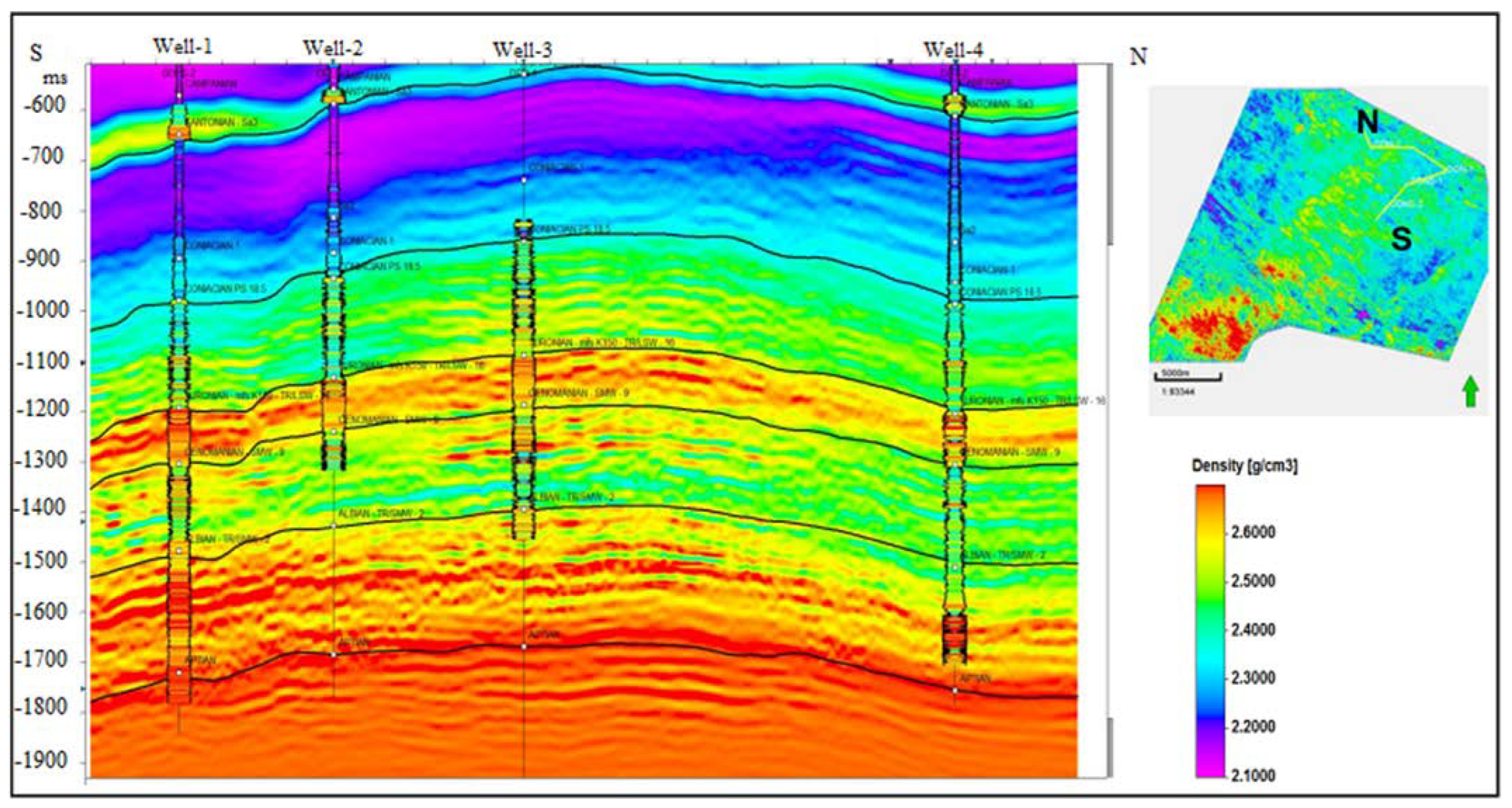
Abstract
1. Introduction
2. Seismic Inversion Model
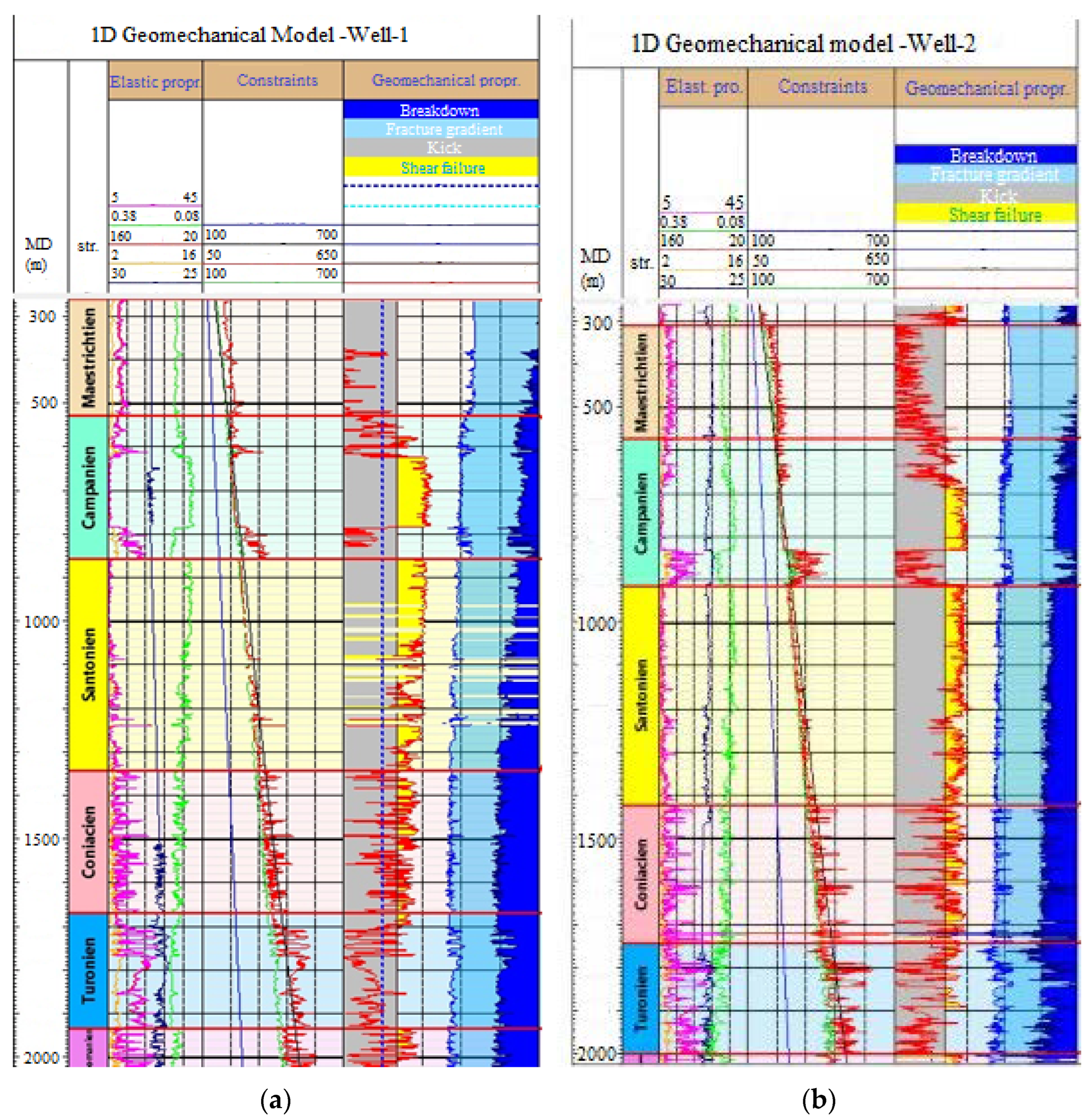
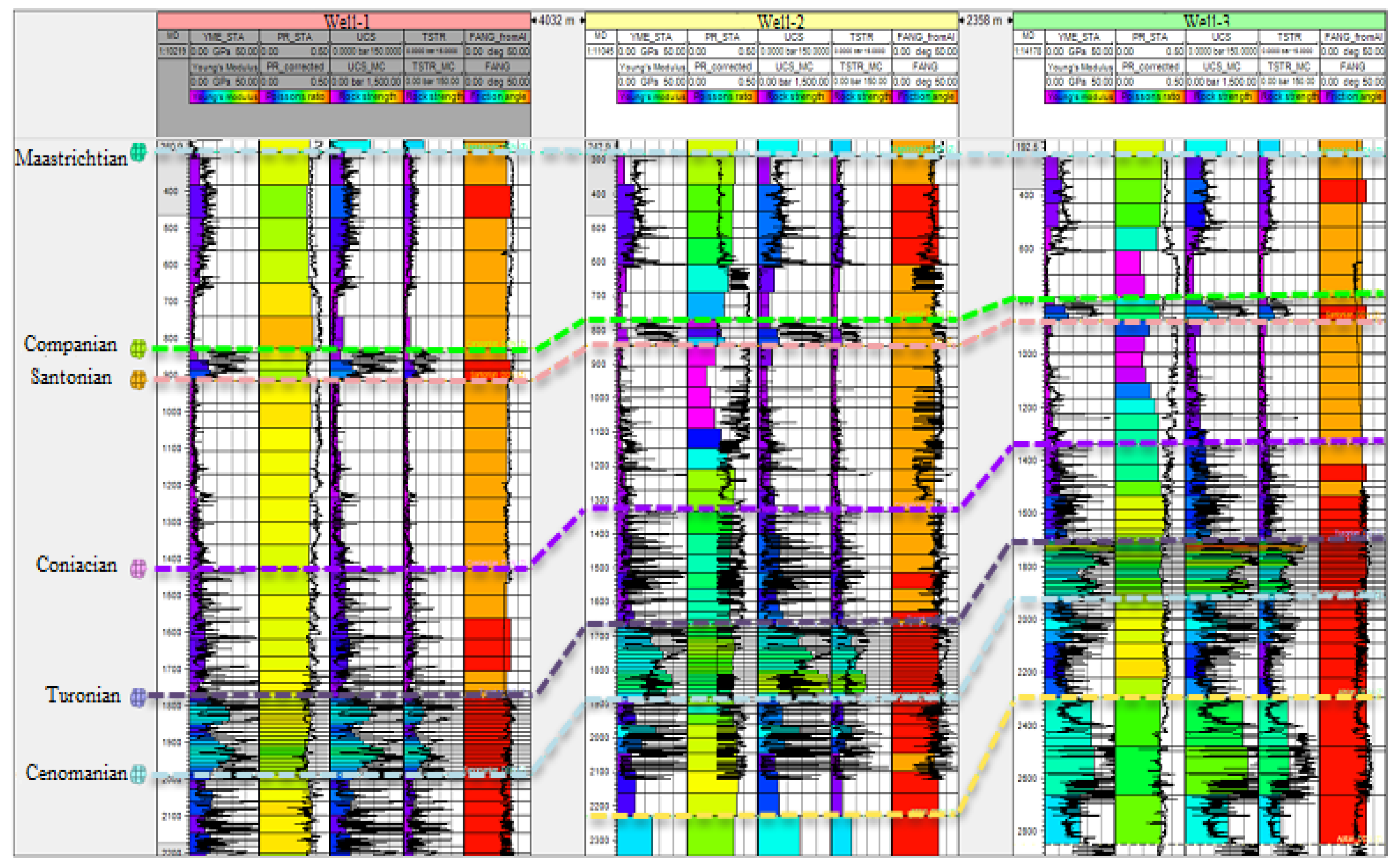
3. 1D Geomechanical Model Construction
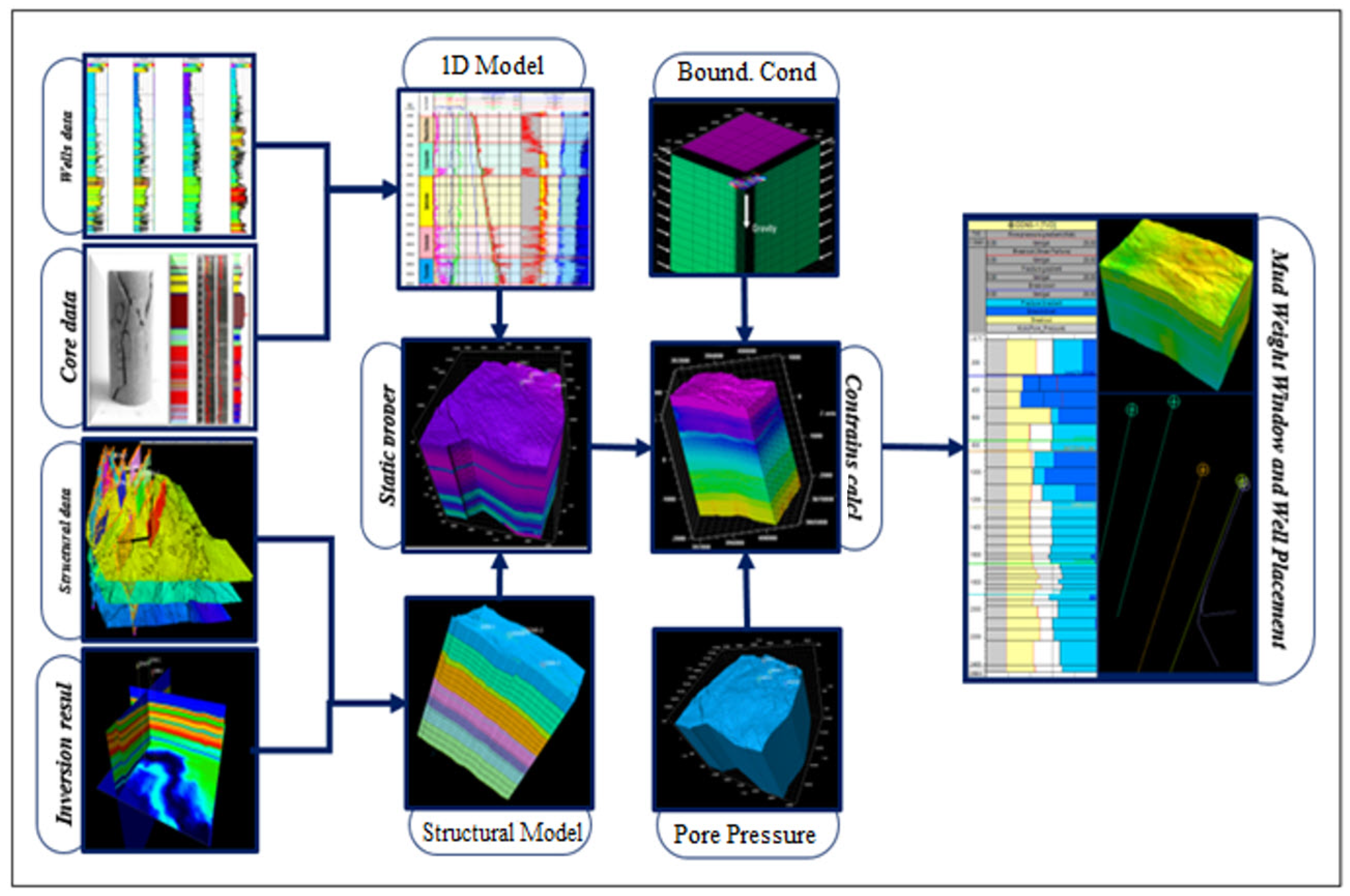
4. Three-Dimensional (3D) Geomechanical Model Construction
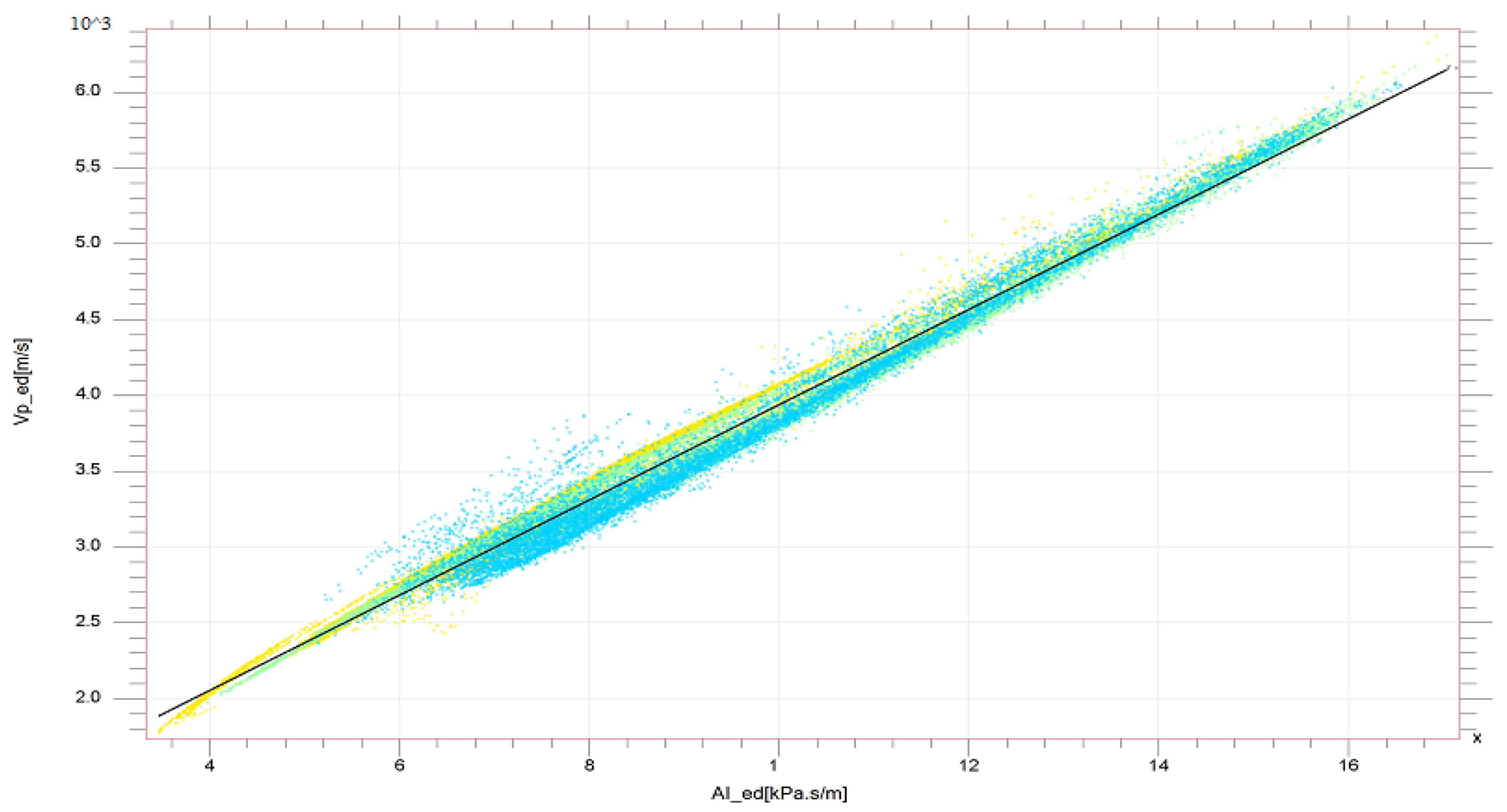
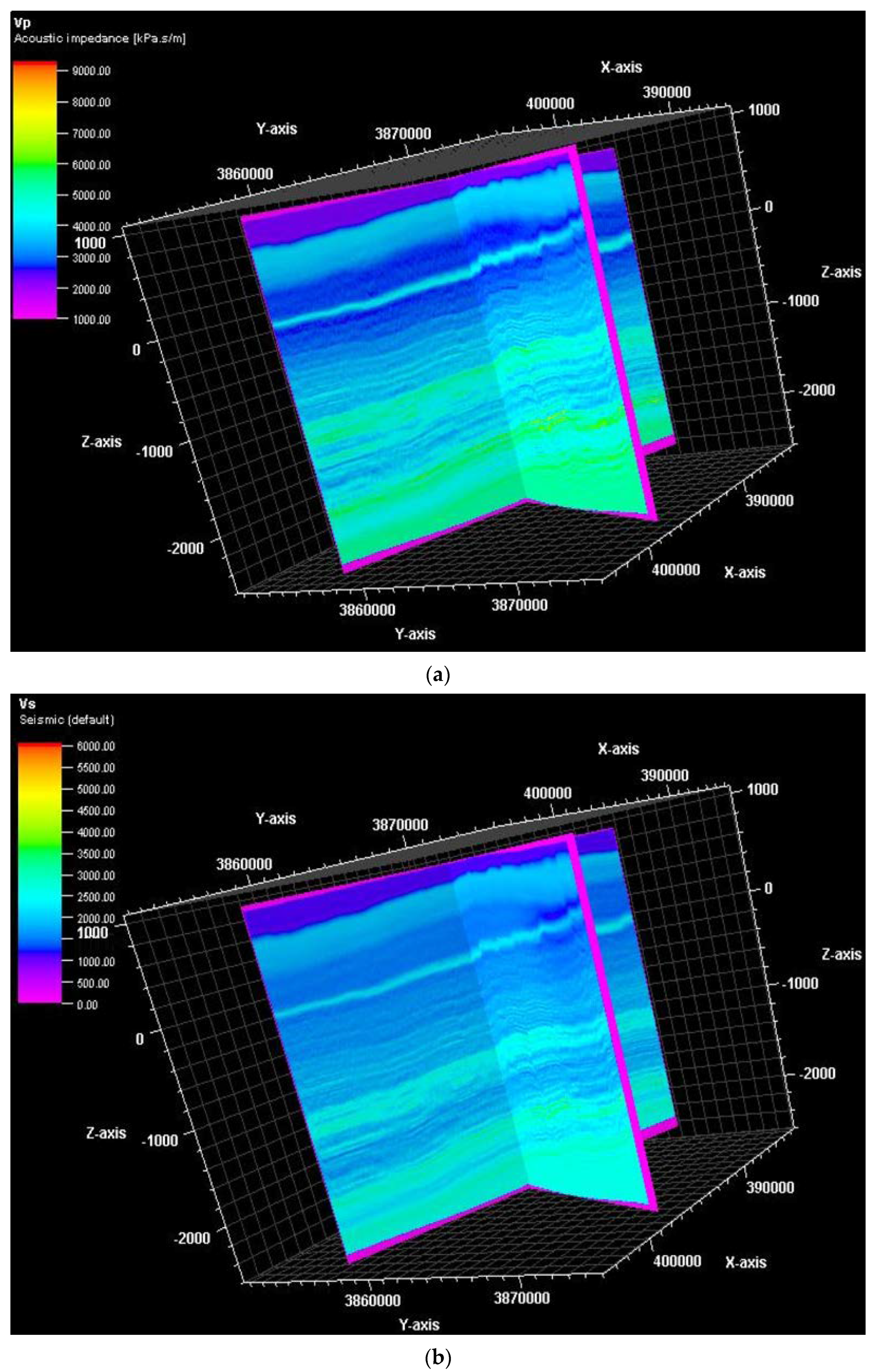
4.1. Generation of Vp and Vs Volumes
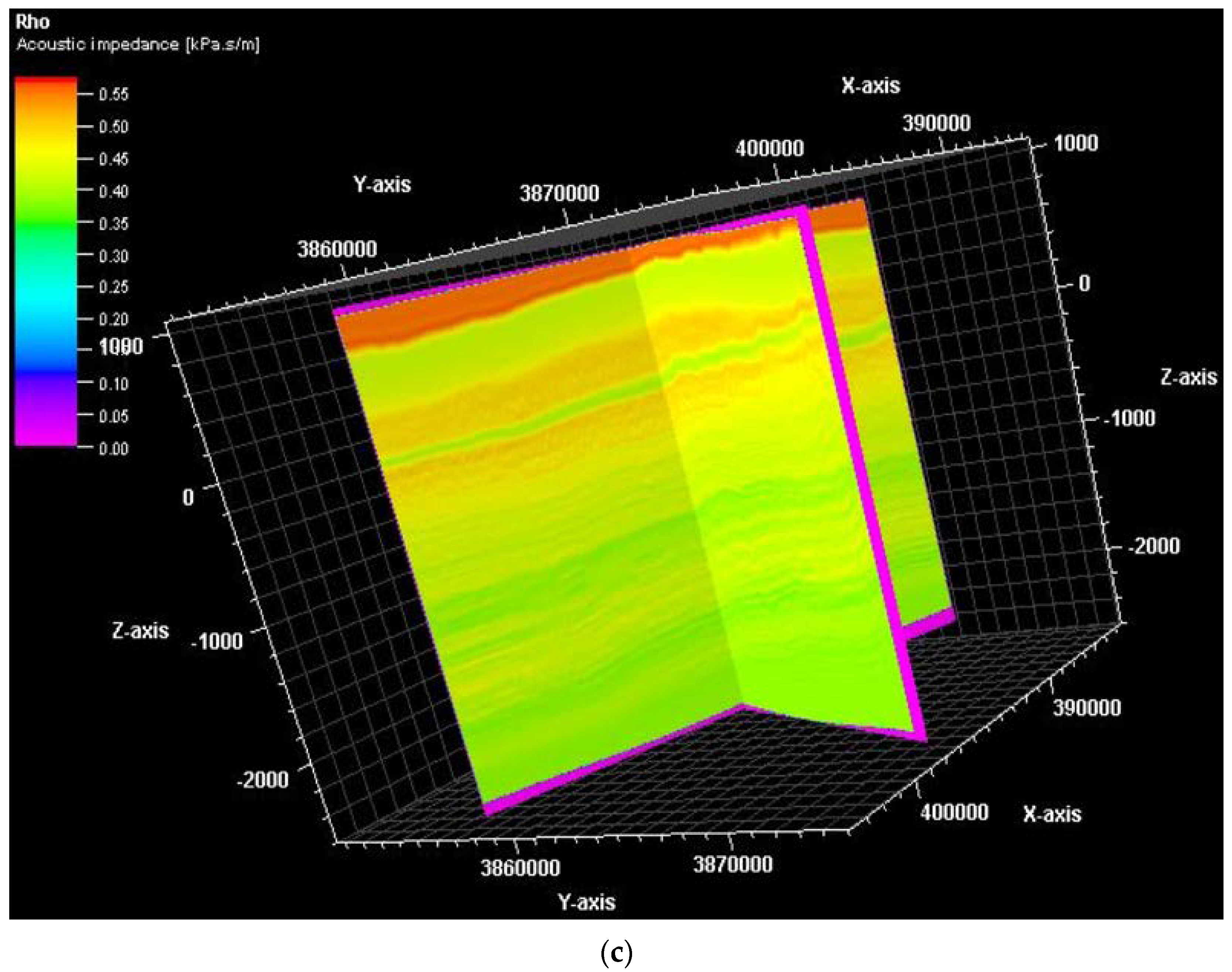
4.2. Density Volume Generation
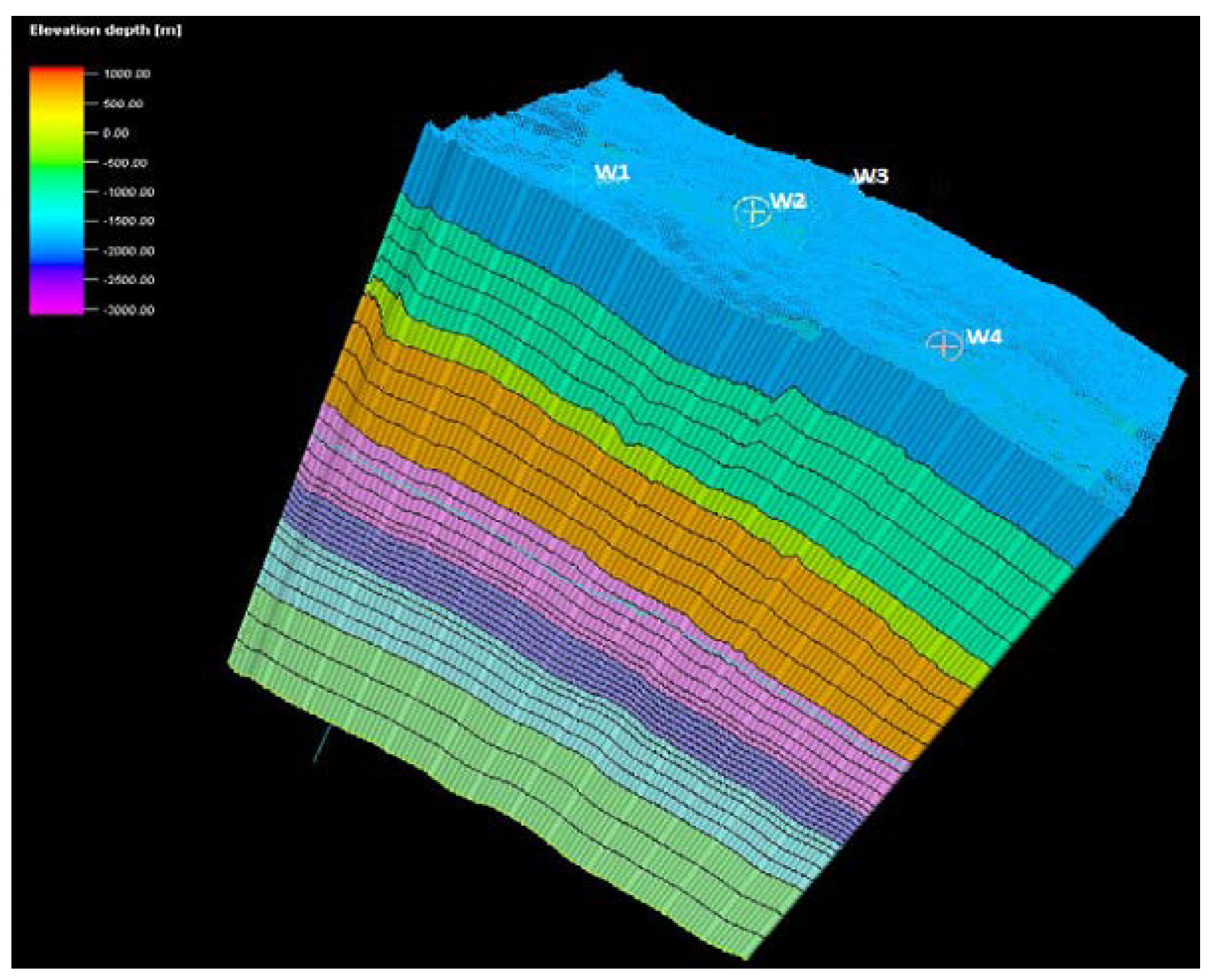
4.3. Digital Grid Creation
4.4. Rock Typing
4.5. Calculation of Limiting Conditions and Constraints
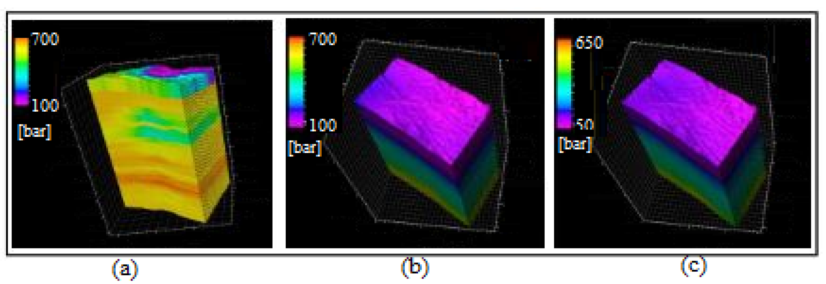
- The vertical stress was determined from the density volume, and it was not quite accurate due to the quality of the seismic data. Nevertheless, the estimated vertical stresses remained close to the real values obtained from core data;
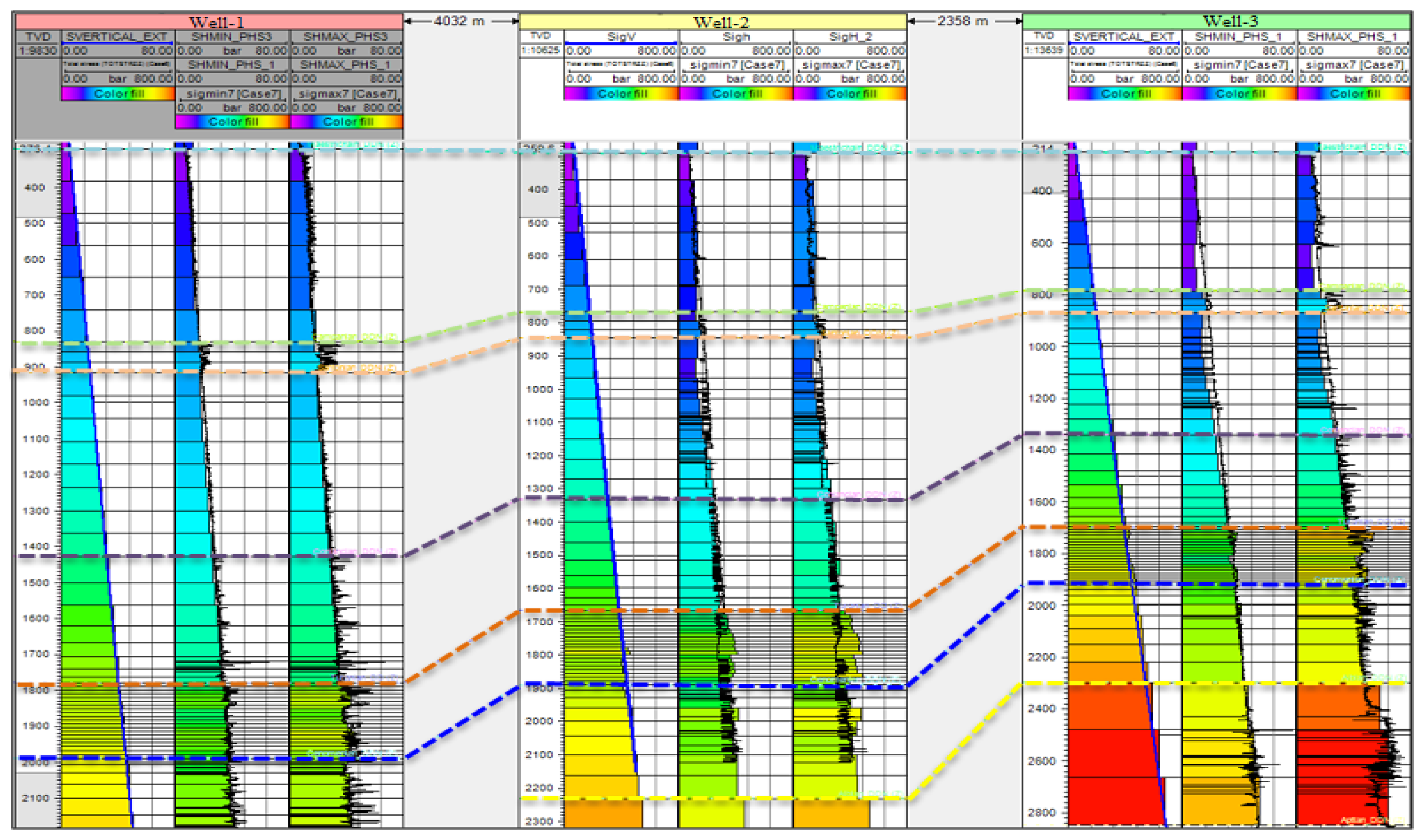
- The horizontal stresses, caused by the effects of tectonics, were estimated from the results of the 1D geomechanical model, which was established at the level of the four wells [30].
5. Well Design
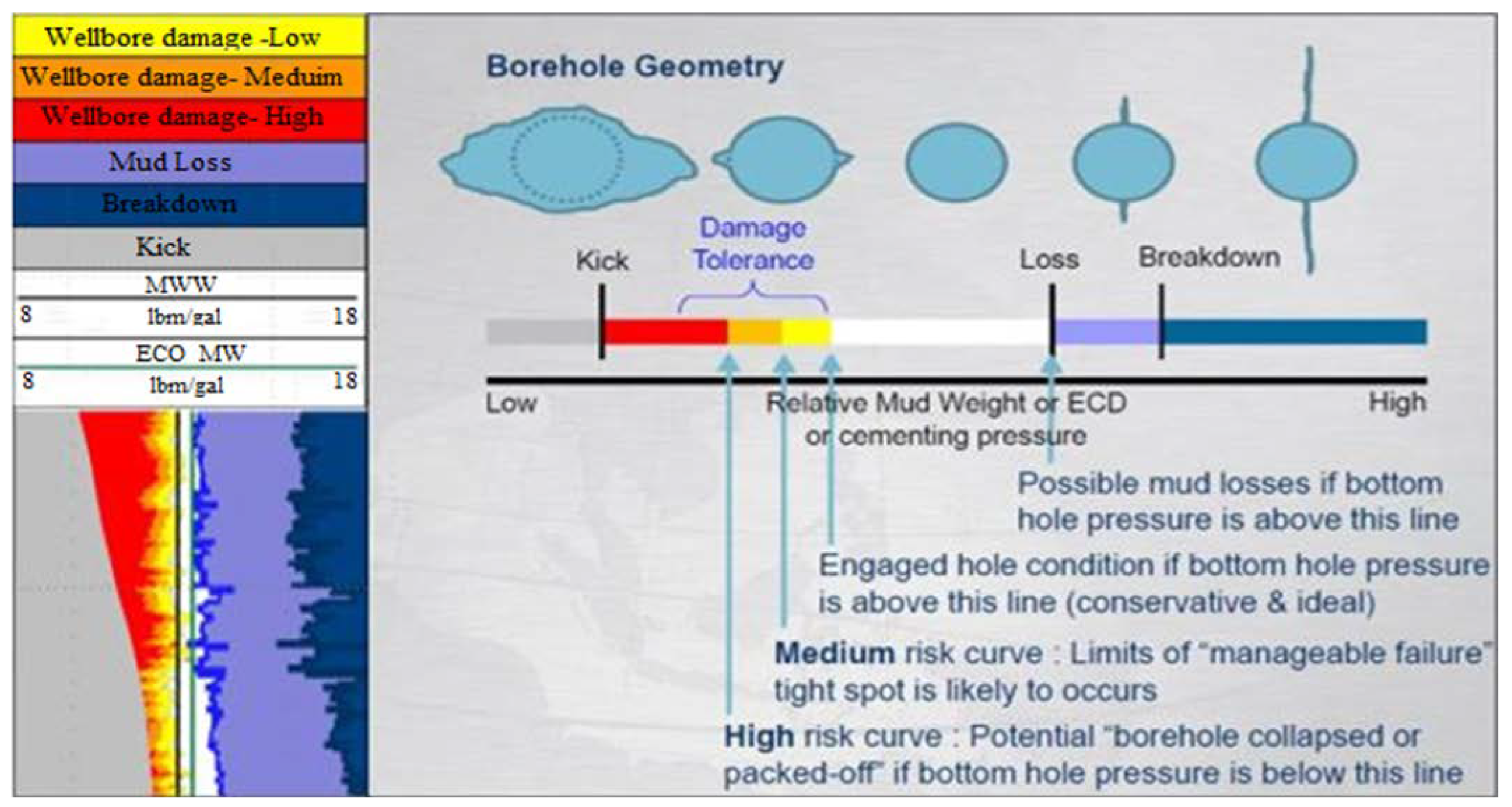
Determination of the Mud Density Window
6. Discussion
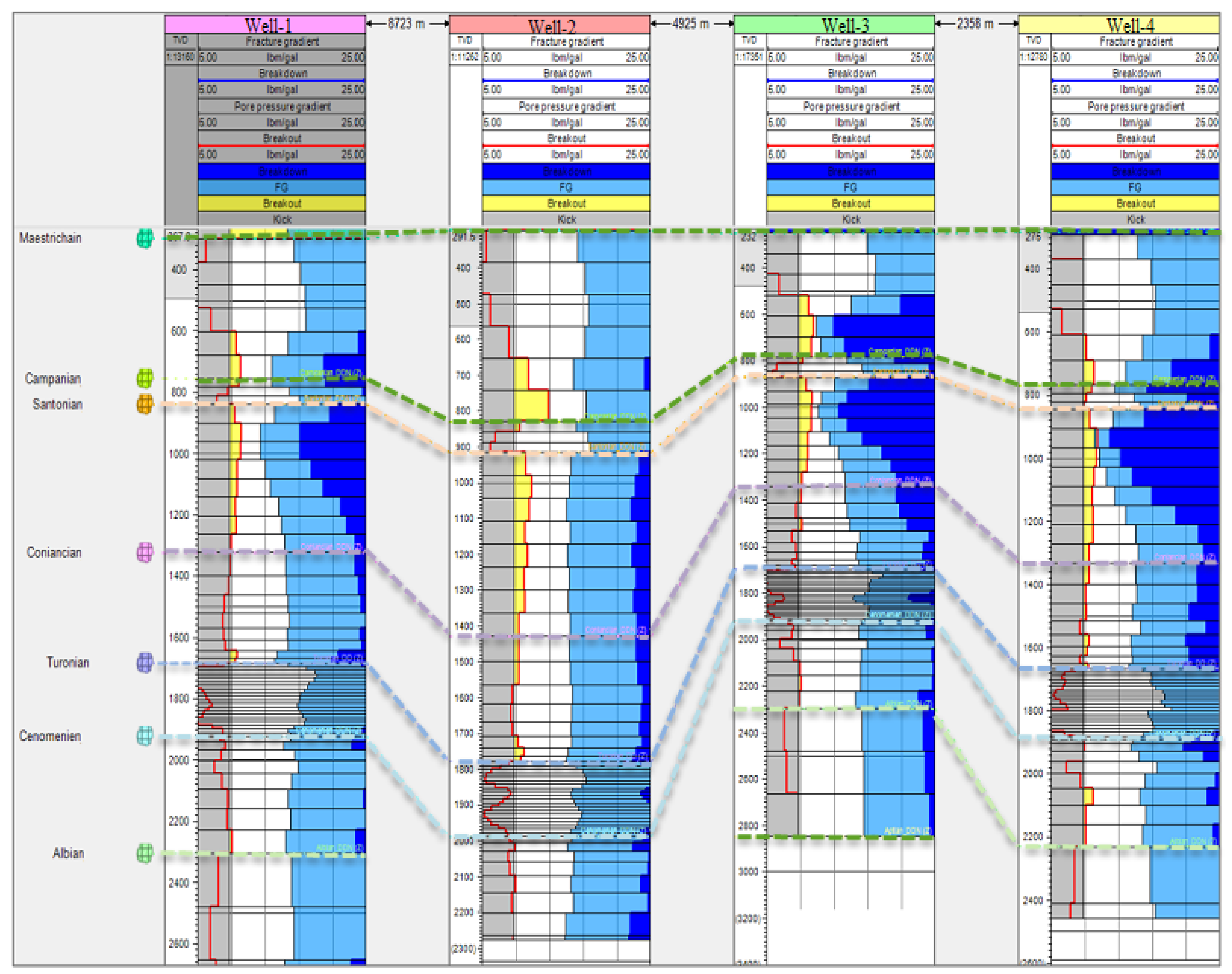
- Gary block: the pore pressure values. If they become higher than the pressure created by the mud density, a kick could occur in the Turonian formation at well 5. The kicks correspond to lower shelling of the walls that that applied by the geological formations around the well
- Yellow block: the fracture limit (shear failure or breakout). This occurs when the mud density is below the maximum in situ stress, but it should be controllable while drilling well 5 [42];
- Light blue block: the fracture gradient limit, which is caused by the minimum horizontal in situ stress. When the mud density is higher than the latter, this will open the existing fractures. This should also be controlled during the drilling of well 5 in order to avoid fracturing the Turonian formation;
- Dark blue block: the breakdown (tensile break). This occurs when the mud density is greater than the maximum horizontal stress. The latter should also be considered when drilling well 5.
7. Conclusions
- In this paper, a 3D geomechanical model was constructed in order to help drillers ensure the stability of the wellbores of hydrocarbon wells without damaging the reservoir in a petroleum field located in the southeast of Algeria;
- The seismic inversion cubes were used as the input data for the construction of the 3D geomechanical model. The 1D geomechanical profiles, generated at the wells’ scales, were used as basic tools for the construction of the 3D geomechanical model;
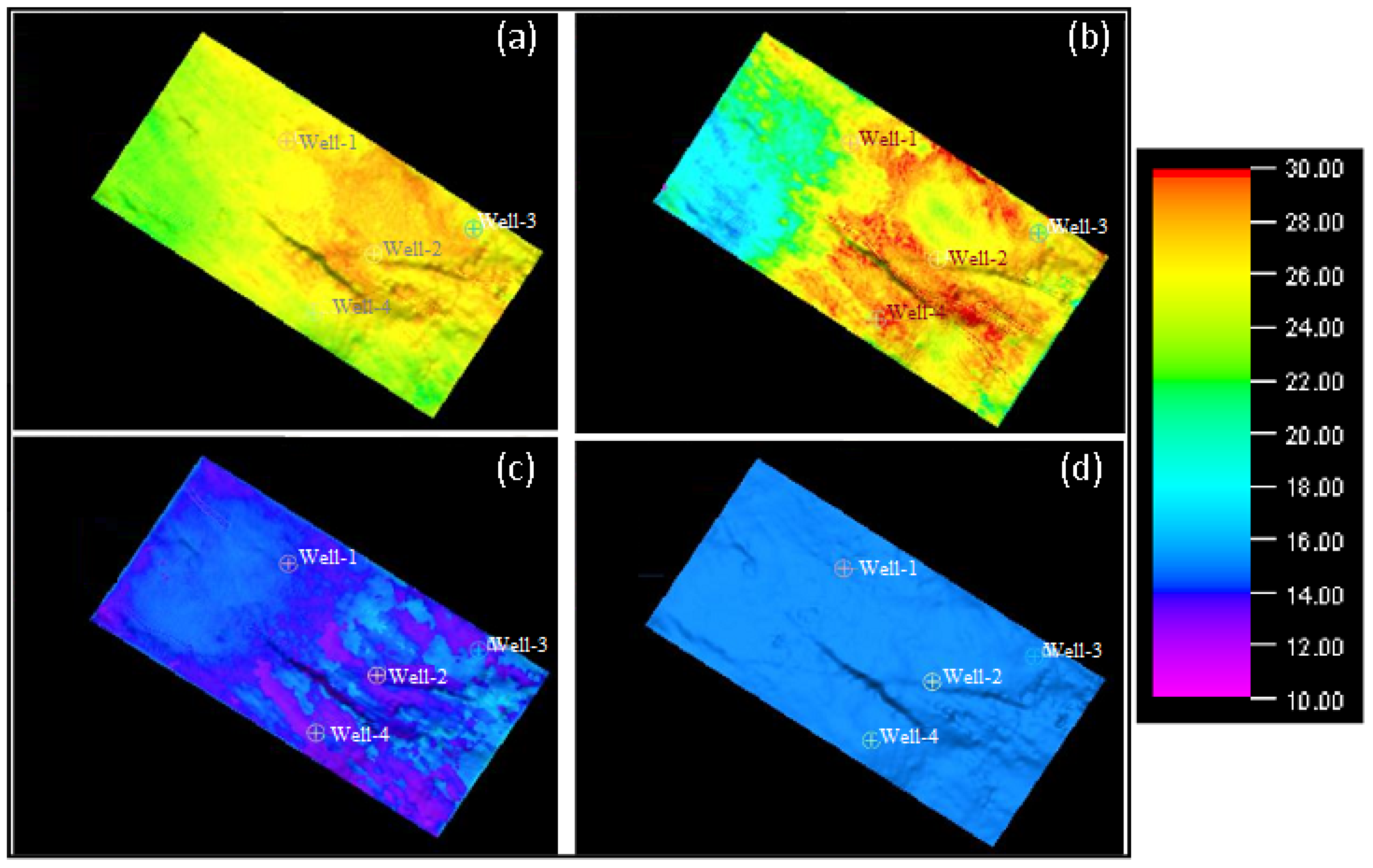
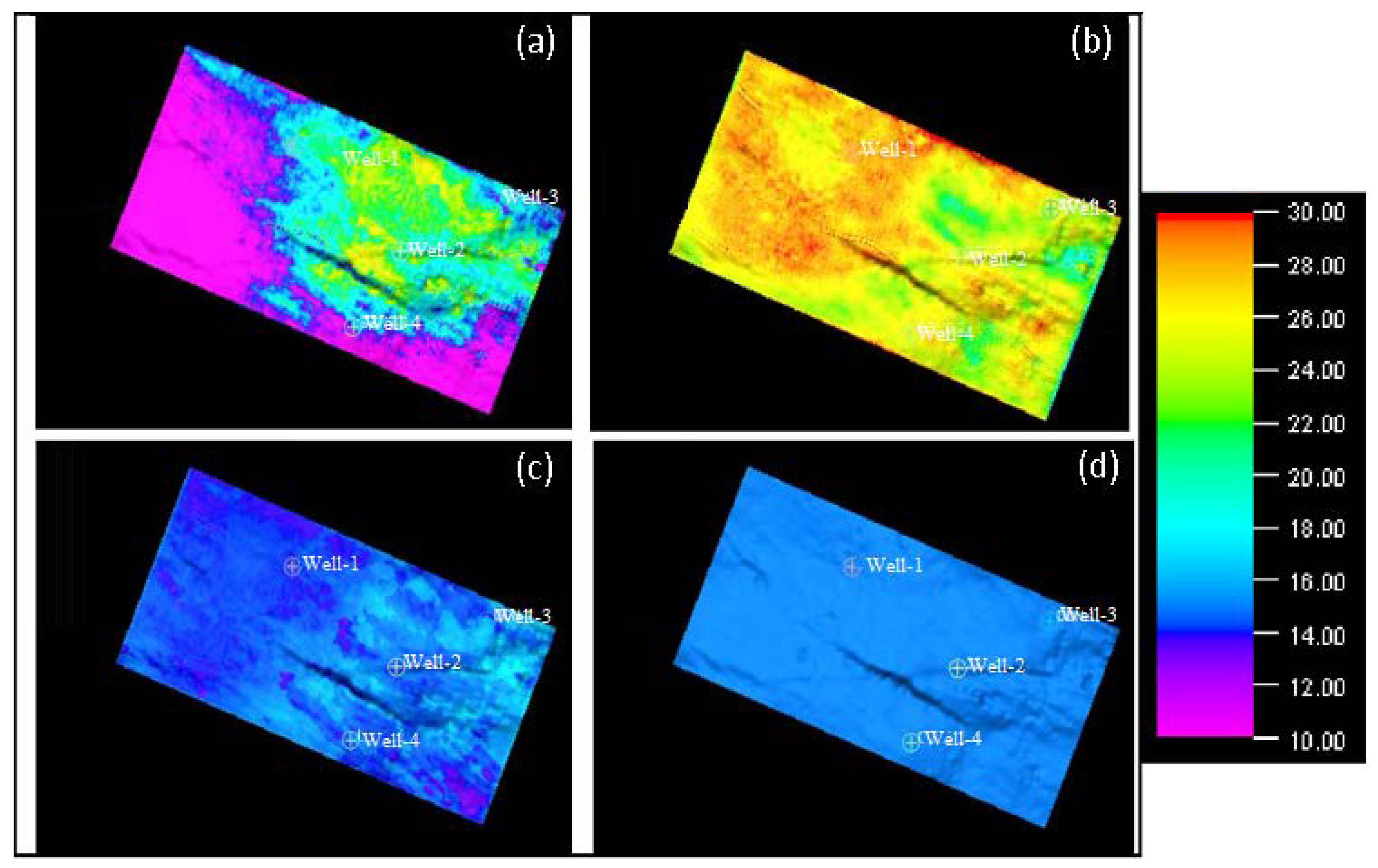
- The 3D geomechanical model provided information on the spatial distribution of the existing stresses in the reservoir and all subjacent layers;
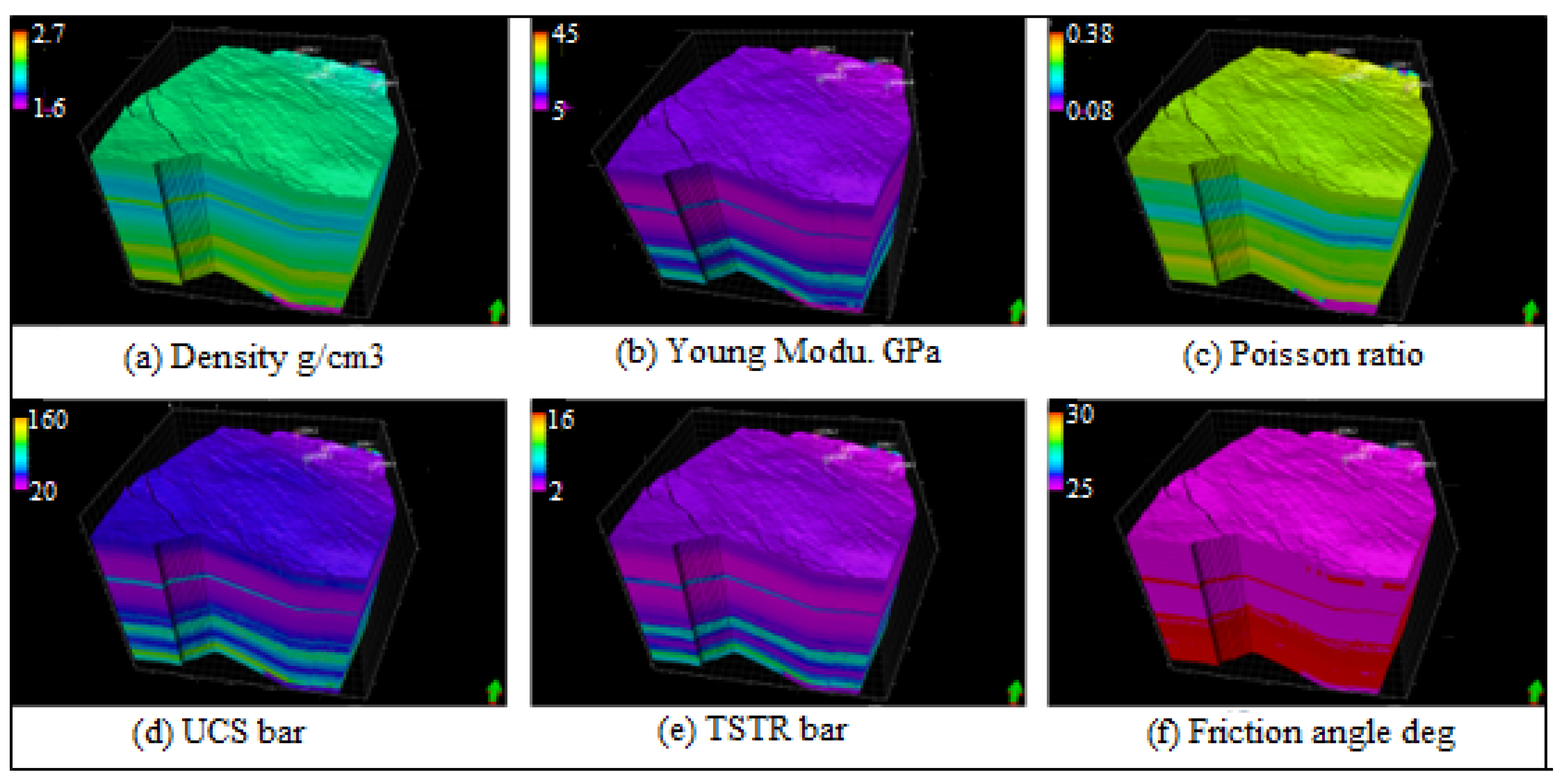
- As a result, this study provides a powerful and reliable tool for drilling new wells and to optimize profitability by avoiding drilling incidents. It allows the estimation of the different mechanical properties of rocks at the seismic scale;
- This is an effective way to determine the mud density to be used when drilling new wells in a studied area, thus allowing the determination of the preferred direction for their boreholes;
- Furthermore, by obtaining such information, simulations of on-going wells can be performed at any position in the volume, and in any direction, so that an estimate of the drilling mud density window can be obtained simultaneously;
- In addition, this model can help drillers choose the location and the optimal direction of new wells with the maximum possible wellbore stability;
- The 3D geomechanical model can be also used to guide hydraulic fracturing supervisors in undertaking fracturing jobs in tight reservoirs based on the robust information on the spatial distribution of stresses, their directions, and their amplitudes.
Author Contributions
Funding
Data Availability Statement
Conflicts of Interest
References
- Ashraf, U.; Zhu, P.; Yasin, Q.; Anees, A.; Imraz, M.; Mangi, H.N.; Shakeel, S. Classification of reservoir facies using well log and 3D seismic attributes for prospect evaluation and field development: A case study of Sawan gas field, Pakistan. J. Pet. Sci. Eng. 2019, 175, 338–351. [Google Scholar] [CrossRef]
- Anees, A.; Zhang, H.; Ashraf, U.; Wang, R.; Liu, K.; Abbas, A.; Ullah, Z.; Zhang, X.; Duan, L.; Liu, F.; et al. Sedimentary Facies Controls for Reservoir Quality Prediction of Lower Shihezi Member-1 of the Hangjinqi Area, Ordos Basin. Minerals 2022, 12, 126. [Google Scholar] [CrossRef]
- Anees, A.; Zhang, H.; Ashraf, U.; Wang, R.; Liu, K.; Mangi, H.N.; Jiang, R.; Zhang, X.; Liu, Q.; Tan, S.; et al. Identification of Favorable Zones of Gas Accumulation via Fault Distribution and Sedimentary Facies: Insights from Hangjinqi Area, Northern Ordos Basin. Front. Earth Sci. 2022, 9, 822670. [Google Scholar] [CrossRef]
- McLean, M.; Addis, M. Wellbore Stability: The Effect of Strength Criteria on Mud Weight Recommendations. In Proceedings of the SPE Annual Technical Conference and Exhibition, New Orleans, Louisiana, 23–26 September 1990. [Google Scholar] [CrossRef]
- Eladj, S.; Lounissi, T.K.; Doghmane, M.Z.; Djeddi, M. Lithological Characterization by Simultaneous Seismic Inversion in Algerian South Eastern Field. Eng. Technol. Appl. Sci. Res. 2020, 10, 5251–5258. [Google Scholar] [CrossRef]
- Qiuguo, L.; Zhang, X.; Al-Ghammari, K.S.; Mohsin, L.; Jiroudi, F.; Al Rawahi, A. 3-D Geomechanical Modeling and Wellbore Stability Analysis in Abu Butabul Field. In Proceedings of the International Petroleum Conference and Exhibition (SPE), Abu Dhabi, United Arab Emirates, 11–14 November 2012. [Google Scholar] [CrossRef]
- Ashraf, U.; Zhang, H.; Anees, A.; Ali, M.; Zhang, X.; Abbasi, S.S.; Mangi, H.N. Controls on Reservoir Heterogeneity of a Shallow-Marine Reservoir in Sawan Gas Field, SE Pakistan: Implications for Reservoir Quality Prediction Using Acoustic Impedance Inversion. Water 2020, 12, 2972. [Google Scholar] [CrossRef]
- Wang, Y.; Ge, Q.; Lu, W.; Yan, X. Well-Logging Constrained Seismic Inversion Based on Closed-Loop Convolutional Neural Network. IEEE Trans. Geosci. Remote Sens. 2020, 58, 5564–5574. [Google Scholar] [CrossRef]
- Fohrmann, M.; Pecher, I. Analysing sand-dominated channel systems for potential gas-hydrate-reservoirs using an AVO seismic inversion technique on the Southern Hikurangi Margin, New Zealand. Mar. Pet. Geol. 2012, 38, 19–34. [Google Scholar] [CrossRef]
- Thanh, H.V.; Lee, K.-K. 3D geo-cellular modeling for Oligocene reservoirs: A marginal field in offshore Vietnam. J. Pet. Explor. Prod. Technol. 2021, 12, 1–19. [Google Scholar] [CrossRef]
- Giroldi, L.; Wallick, B.; Rodriguez-Herrera, A.; Koutsabeloulis, N.; Lowden, D. Applications of broadband seismic inversion in the assessment of drilling and completion strategies: A case study from eastern Saudi Arabia. SEG Tech. Program Expand. Abstr. 2014, 2014, 3153–3156. [Google Scholar] [CrossRef]
- Thanh, H.V.; Sugai, Y.; Sasaki, K. Impact of a new geological modelling method on the enhancement of the CO2 storage assessment of E sequence of Nam Vang field, offshore Vietnam. Energy Sources Part A Recover. Util. Environ. Eff. 2020, 42, 1499–1512. [Google Scholar] [CrossRef]
- Hale, A.H.; Mody, F.K.; Salisbury, D.P. The Influence of Chemical Potential on Wellbore Stability. SPE Drill. Complet. 1993, 8, 207–216. [Google Scholar] [CrossRef]
- Thanh, H.V.; Sugai, Y.; Nguele, R.; Sasaki, K. Integrated workflow in 3D geological model construction for evaluation of CO2 storage capacity of a fractured basement reservoir in Cuu Long Basin, Vietnam. Int. J. Greenh. Gas Control 2019, 90, 102826. [Google Scholar] [CrossRef]
- Thanh, H.V.; Sugai, Y. Integrated modelling framework for enhancement history matching in fluvial channel sandstone reservoirs. Upstream Oil Gas Technol. 2021, 6, 100027. [Google Scholar] [CrossRef]
- Yanghua, W. Seismic Inversion: Theory and Applications; Wiley Blackwell, John Whiler & Sons: Hoboken, NJ, USA, 2007; ISBN 9781119258025. [Google Scholar]
- Eladj, S.; Lounissi, T.K.; Doghmane, M.Z.; Djeddi, M. Wellbore Stability Analysis Based on 3D Geo-Mechanical Model of an Algerian Southeastern Field. In Advances in Geophysics, Tectonics and Petroleum Geosciences. CAJG 2019. Advances in Science, Technology & Innovation; Springer: Berlin/Heidelberg, Germany, 2022. [Google Scholar] [CrossRef]
- Boualam, A.; Rasouli, V.; Dalkhaa, C.; Djezzar, S. Stress-Dependent Permeability and Porosity in Three Forks Carbonate Reservoir, Williston Basin. In Proceedings of the Paper 54th U.S. Rock Mechanics/Geomechanics Symposium, Physical Event Cancelled, Golden, CO, USA, 28 June–1 July 2020. [Google Scholar]
- Bacetti, A.; Doghmane, M. A Practical Workflow Using Seismic Attributes to Enhance Sub Seismic Geological Structures and Natural Fractures Correlation. In Proceedings of the First EAGE Digitalization Conference and Exhibition, Vienna, Austria, 30 November–3 December 2020; Volume 2020, pp. 1–5. [Google Scholar] [CrossRef]
- Doghmane, M.Z.; Ouadfeul, S.A.; Benaissa, Z.; Eladj, S. Classification of Ordovician Tight Reservoir Facies in Algeria by Using Neuro-Fuzzy Algorithm. In Artificial Intelligence and Heuristics for Smart Energy Efficiency in Smart Cities. IC-AIRES 2021. Lecture Notes in Networks and Systems; Hatti, M., Ed.; Springer: Berlin/Heidelberg, Germany, 2021; Volume 361. [Google Scholar] [CrossRef]
- Gray, D.; Anderson, P.; Logel, J.; Delbecq, F.; Schmidt, D.; Schmid, R. Estimation of stress and geomechanical properties using 3D seismic data. First Break 2012, 30, 59–68. [Google Scholar] [CrossRef]
- Riaz, M.S.; Bin, S.; Naeem, S.; Kai, W.; Xie, Z.; Gilani SM, M.; Ashraf, U. Over 100 years of faults interaction, stress accumulation, and creeping implications, on Chaman Fault System, Pakistan. Int. J. Earth Sci. 2019, 108, 1351–1359. [Google Scholar] [CrossRef]
- Djezzar, S.; Rasouli, V.; Boualam, A.; Rabiei, M. An integrated workflow for multiscale fracture analysis in reservoir analog. Arab. J. Geosci. 2020, 13, 161. [Google Scholar] [CrossRef]
- Neves, F.A.; Al-Marzoug, A.; Kim, J.J.; Nebrija, E.L. Fracture characterization of deep tight gas sands using azimuthal velocity and AVO seismic data in Saudi Arabia. Lead. Edge 2003, 22, 469–475. [Google Scholar] [CrossRef]
- Boualam, A.; Djezzar, S.; Rasouli, V.; Rabiei, M. 3D Modeling and Natural Fractures Characterization in Hassi Guettar Field, Algeria. In Proceedings of the 53rd U.S. Rock Mechanics/Geomechanics Symposium, New York, NY, USA, 23–26 June 2019. [Google Scholar]
- Duffaut, K.; Landrø, M. Vp/Vs ratio versus differential stress and rock consolidation—A comparison between rock models and time-lapse AVO data. Geophysics 2007, 72, C81–C94. [Google Scholar] [CrossRef]
- Xiao, X.; Jenakumo, T.; Ash, C.; Bui, H.; Fakunle, O.; Weaver, S. An Integrated Workflow Combining Seismic Inversion and 3D Geomechanics Modeling—Bonga Field, Offshore Nigeria. In Proceedings of the Offshore Technology Conference, Houston, TX, USA, 2–5 May 2016. [Google Scholar] [CrossRef]
- Sengupta, M.; Dai, J.; Volterrani, S.; Dutta, N.; Rao, N.S.; Al-Qadeeri, B.; Kidambi, V.K. Building a seismic-driven 3D geomechanical model in a deep carbonate reservoir. In Proceedings of the SEG Technical Program Expanded Abstracts 2011, San Antonio, TX, USA, 18–23 September 2011; pp. 2069–2073. [Google Scholar] [CrossRef]
- Trudeng, T.; Garcia-Teijeiro, X.; Rodriguez-Herrera, A.; Khazanehdari, J. Using Stochastic Seismic Inversion as Input for 3D Geomechanical Models. In Proceedings of the IPTC 2014: International Petroleum Technology Conference, Doha, Qatar, 10–12 December 2014; Volume 2014, pp. 1–6, EAGE. [Google Scholar] [CrossRef]
- Ranjbar, A.; Hassani, H.; Shahriar, K. 3D geomechanical modeling and estimating the compaction and subsidence of Fahlian reservoir formation (X-field in SW of Iran). Arab. J. Geosci. 2017, 10, 116. [Google Scholar] [CrossRef]
- Eladj, S.; Doghmane, M.Z.; Aliouane, L.; Ouadfeul, S.-A. Porosity Model Construction Based on ANN and Seismic Inversion: A Case Study of Saharan Field (Algeria). In Advances in Geophysics, Tectonics and Petroleum Geosciences. CAJG 2019. Advances in Science, Technology & Innovation; Springer: Berlin/Heidelberg, Germany, 2022. [Google Scholar] [CrossRef]
- Convers, C. Prediction of Reservoir Properties for Geomechanical Analysis Using 3-D Seismic Data and Rock Physics Modeling in the Vaca Muerta Formation, Neuquén Basin, Argentina. Ph.D. Thesis, Colorado School of Mines, Golden, CO, USA, 2017. [Google Scholar]
- Ashraf, U.; Zhang, H.; Anees, A.; Mangi, H.N.; Ali, M.; Zhang, X.; Imraz, M.; Abbasi, S.S.; Abbas, A.; Ullah, Z.; et al. A Core Logging, Machine Learning and Geostatistical Modeling Interactive Approach for Subsurface Imaging of Lenticular Geobodies in a Clastic Depositional System, SE Pakistan. Nonrenewable Resour. 2021, 30, 2807–2830. [Google Scholar] [CrossRef]
- Alalimi, A.; AlRassas, A.M.; Thanh, H.V.; Al-Qaness, M.A.A.; Pan, L.; Ashraf, U.; Al-Alimi, D.; Moharam, S. Developing the efficiency-modeling framework to explore the potential of CO2 storage capacity of S3 reservoir, Tahe oilfield, China. Géoméch. Geophys. Geo-Energy Geo-Resour. 2022, 8, 128. [Google Scholar] [CrossRef]
- Cherana, A.; Aliouane, L.; Doghmane, M.; Ouadfeul, S.-A. Fuzzy Clustering Algorithm for Lithofacies Classification of Ordovician Unconventional Tight Sand Reservoir from Well-Logs Data (Algerian Sahara). In Advances in Geophysics, Tectonics and Petroleum Geosciences. CAJG 2019. Advances in Science, Technology & Innovation; Springer: Berlin/Heidelberg, Germany, 2022. [Google Scholar] [CrossRef]
- Berryman, J.G. Origin of Gassmann’s equations. Geophysics 1999, 64, 1627–1629. [Google Scholar] [CrossRef]
- Goodway, B.; Perez, M.; Varsek, J.; Abaco, C. Seismic petrophysics and isotropic-anisotropic AVO methods for unconventional gas exploration. Lead. Edge 2010, 29, 1500–1508. [Google Scholar] [CrossRef]
- Doghmane, M.Z.; Belahcene, B.; Kidouche, M. Application of Improved Artificial Neural Network Algorithm in Hydrocarbons’ Reservoir Evaluation. In Renewable Energy for Smart and Sustainable Cities. Lecture Notes in Networks and Systems 62; Hatti, M., Ed.; Springer: Berlin/Heidelberg, Germany, 2018; pp. 129–138. [Google Scholar] [CrossRef]
- Correa, A.C.F.; Newman, R.B.; Naveira, V.P.; de Souza, A.L.S.; Araujo, T.; da Silva, A.A.C.; Soares, A.C.; Herwanger, J.V.; Meurer, G.B. Integrated Modeling for 3D Geomechanics and Coupled Simulation of Fractured Carbonate Reservoir. In Proceedings of the Offshore Technology Conference, OTC Brasil, Rio de Janeiro, Brazil, 29–31 October 2013. [Google Scholar] [CrossRef]
- Po, C.; Lee, E.-J. Full-3D Seismic Waveform Inversion: Theory, Software and Practice, Springer Geophysics; Springer International Publishing: Berlin/Heidelberg, Germany, 2015; ISBN 978-3-319-16603-2. [Google Scholar] [CrossRef]
- Cheatham, J.J., Jr. Wellbore Stability. J. Pet. Technol. 1984, 36, 889–896. [Google Scholar] [CrossRef]
- Djezzar, S.; Rasouli, V.; Boualam, A.; Rabiei, M. Size Scaling and Spatial Clustering of Natural Fracture Networks Using Fractal Analysis. In Proceedings of the 53rd U.S. Rock Mechanics/Geomechanics Symposium, New York, NY, USA, 23–26 June 2019. [Google Scholar]
- Eladj, S.; Doghmane, M.Z.; Belahcene, B. Design of New Model for Water Saturation Based on Neural Network for Low-Resistivity Phenomenon (Algeria). In Advances in Geophysics, Tectonics and Petroleum Geosciences. CAJG 2019. Advances in Science, Technology & Innovation; Springer: Berlin/Heidelberg, Germany, 2022. [Google Scholar] [CrossRef]


Publisher’s Note: MDPI stays neutral with regard to jurisdictional claims in published maps and institutional affiliations. |
© 2022 by the authors. Licensee MDPI, Basel, Switzerland. This article is an open access article distributed under the terms and conditions of the Creative Commons Attribution (CC BY) license (https://creativecommons.org/licenses/by/4.0/).
Share and Cite
Eladj, S.; Doghmane, M.Z.; Lounissi, T.K.; Djeddi, M.; Tee, K.F.; Djezzar, S. 3D Geomechanical Model Construction for Wellbore Stability Analysis in Algerian Southeastern Petroleum Field. Energies 2022, 15, 7455. https://doi.org/10.3390/en15207455
Eladj S, Doghmane MZ, Lounissi TK, Djeddi M, Tee KF, Djezzar S. 3D Geomechanical Model Construction for Wellbore Stability Analysis in Algerian Southeastern Petroleum Field. Energies. 2022; 15(20):7455. https://doi.org/10.3390/en15207455
Chicago/Turabian StyleEladj, Said, Mohamed Zinelabidine Doghmane, Tanina Kenza Lounissi, Mabrouk Djeddi, Kong Fah Tee, and Sofiane Djezzar. 2022. "3D Geomechanical Model Construction for Wellbore Stability Analysis in Algerian Southeastern Petroleum Field" Energies 15, no. 20: 7455. https://doi.org/10.3390/en15207455
APA StyleEladj, S., Doghmane, M. Z., Lounissi, T. K., Djeddi, M., Tee, K. F., & Djezzar, S. (2022). 3D Geomechanical Model Construction for Wellbore Stability Analysis in Algerian Southeastern Petroleum Field. Energies, 15(20), 7455. https://doi.org/10.3390/en15207455