Analysis of Deep Learning Neural Networks for Seismic Impedance Inversion: A Benchmark Study

Abstract

Neural networks have been applied to seismic inversion problems since the 1990s. More recently, many publications have reported the use of Deep Learning (DL) neural networks capable of performing seismic inversion with promising results. However, when solving a seismic inversion problem with DL, each author uses, in addition to different DL models, different datasets and different metrics for performance evaluation, which makes it difficult to compare performances. Depending on the data used for training and the metrics used for evaluation, one model may be better or worse than another. Thus, it is quite challenging to choose the appropriate model to meet the requirements of a new problem. This work aims to review some of the proposed DL methodologies, propose appropriate performance evaluation metrics, compare the performances, and observe the advantages and disadvantages of each model implementation when applied to the chosen datasets. The publication of this benchmark environment will allow fair and uniform evaluations of newly proposed models and comparisons with currently available implementations.

1. Introduction

Seismic inversion extracts quantitative reservoir rock and fluid properties from seismic reflection data [1]. Seismic reflection data are geophysical records obtained from the reflection of acoustic waves in the subsurface due to the different properties of the rocks and fluids contained therein. Seismic waves are artificially generated at the surface by a controlled energy source and their reflections are captured by sensors. These signals are then processed to create a seismic record [2,3].

There are two types of seismic inversion: stochastic and deterministic. In general, seismic inversion, in addition to reflection data, typically includes other reservoir measurements such as well logs and cores. Stochastic seismic inversion is a statistical process integrating well and seismic data, which generates multiple realizations. Deterministic seismic inversion returns only one realization, considered “optimal” [4]. In most cases, the seismic inversion problem is not well posed, i.e., it is not a linear problem with a single solution. Thus, different combinations of rocks and waves generate the same seismic record [1].

The applications of seismic inversion helps to predict rock and fluid properties that are needed for subsurface studies, allowing the construction of a detailed 3D petrophysical model [5]. In the gas and oil industry, seismic inversion is one of the most frequently used methods for reservoir characterization. It is essential to reduce the necessity for well drilling, which is an expensive and time-consuming process [6].

The more traditional approaches in seismic inversion involve creating rock models, testing their adherence to the obtained data, adjusting the model, and continuing iteratively until a satisfactory model is obtained. However, the neural network approach is much simpler, requiring only that the input and output sets are known for training the network and sparing the need to create rock models.

Neural networks have been used in geosciences since the 1960s and for seismic inversion particularly since at least the 1990s [7]. Different architectures of neural networks have been used to solve several problems related to seismic inversion, for example, generative adversarial networks in [3,8], variational autoencoders in [9], and convolutional neural networks in [10]. Neural networks have been essential for solving the computational problem of seismic inversions, although the verification method for each approach differs. However, no comprehensive studies were found that evaluate the possibilities of the inversion via a realistic benchmark.

Therefore, in this work, we aim to test several available neural network implementations in a test environment, attempting to replicate real conditions as closely as possible. We selected two datasets based on real environments, where the inputs and outputs of the datasets are known, to test which neural network implementation provides the best seismic inversion, resulting in the best correlation with the expected output. In addition to comparing the results, we describe each neural network implementation in a way that makes it possible to measure the results and the quality of the inversion and also to understand the architectural decisions that lead to such results, thus assisting the development of future studies.

This paper is organized as follows. Section 2 shows the architecture behind some Deep Learning (DL) models and briefly discusses reflection seismology and acoustic impedance. In Section 3, we show some of the available DL implementations mentioned in the previous section and discuss their experiments and results. Section 4 is dedicated to explaining the preparation of our study environment, Section 5 presents the results of the experiments, and Section 6 discusses the obtained results. Section 7 concludes the paper.

2. Theoretical Foundations

In this section, we briefly review some basic concepts necessary for a complete understanding of this research. Initially, we review the concepts of reflection seismology, acoustic impedance, and seismic inversion. Subsequently, we present the Deep Learning neural network models that are reviewed and implemented in our benchmark environment. All these concepts serve as the theoretical basis for our work.

2.1. Reflection Seismology

Reflection seismology is the method used to explore the subsurface properties using reflected waves generated by a pulse on the surface and reflected by interfaces between different types of material in the subsoil. Reflection seismology is performed using tools that generate artificial energy waves from the surface. These waves propagate through the materials (i.e., water or rock) until they reach a significant variation in the material density. Then, part of the energy of these waves is reflected back to the surface, and the other part is refracted until it finds another change and is reflected to the surface from there. Sensors capture the reflected energy portions and later serve as input for seismic inversion methods.

2.2. Acoustic Impedance

Acoustic impedance is a quantity related to the difficulty that a sound wave encounters when propagating through a material and depends upon the speed at which the wave travels and the density of the material. Although it is an acoustic characteristic, the impedance is strongly related to the petroelastic properties of the material [11]. Equation (1) shows the acoustic impedance, given by:

$$\mathrm{Z}=\rho V,$$

(1)

where Z is the acoustic impedance, $\rho$ is the density, and V is the wave propagation velocity.

2.3. Seismic Inversion

Currently, most seismic inversion methods are based on forward modeling convolution. Assuming a convolutional model for the observed seismic trace $s(t)$, we can describe it as:

$$s(t)=r(t)\ast w(t),$$

(2)

where ∗ is the convolutional operator, $r(t)$ is the reflectivity, and $w(t)$ is the wavelet. The goal of seismic inversion is to find the inverse operator $v(t)$ which, convolved with the seismic trace $s(t)$, gives the reflection coefficient. As mentioned in the previous subsection, seismic impedance is strongly related to the material’s properties. Therefore, it is possible to recover the impedance from the reflection coefficient [12].

As described in [13,14], seismic inversion is typically performed in four steps:

• Generation of the subsurface model. A 3D model structure is needed for seismic inversion. The model structure is created by integrating interpreted horizons, faults, and well data. When the 3D model has been created, it is populated with geophysical information from the well logs, such as porosity, density, and velocity. Then, the information in the well is interpolated through the layers of the 3D structure model. Thus, a 3D volume of low frequency is created that represents the interpolated acoustic impedance logs in the subsurface. In addition, this volume can be convoluted with a wavelet to obtain a 3D set of synthetic seismic traces.
• Wavelet extraction. The wavelet can be extracted from the seismic data by taking several seismic traces around the well location and minimizing the misfit between the seismic data and well data.
• Inversion. There are several inversion algorithms such as recursive inversion and constrained sparse spike inversion [15]. The process runs iteratively until the defined best solution is achieved.
• Trace merging. The final step involves merging a low-frequency component extracted from the subsurface model from step 1 with the result of the inversion. This is usually performed to optimize the results of the inversion method chosen in the previous step.

Therefore, seismic inversion is a laborious process, dependent on each step. However, the neural network approach is much simpler, requiring only that the input and output datasets for training the network are known and sparing the need to create the low-frequency model and perform wavelet extraction and trace merging, for example. This approach has shown that the neural network architecture can extract information from the training dataset.

2.4. Summary of DL Models

Before we discuss the Deep Learning neural network models in detail, we briefly discuss the advantages and disadvantages of each one. Figure 1 shows a schematic of their architectures.

Figure 1. Schematics of some Deep Learning network architectures: (a) Convolutional Neural Network (CNN) model with three convolutional layers; (b) Long Short-Term Memory (LSTM) model with three memory blocks (a schematic of a memory block can be seen in Figure 2); (c) Temporal Convolutional Network (TCN) model with three temporal blocks (a schematic of a temporal block can be seen in Figure 3a); (d) Generative Adversary Network (GAN) model with a generator and a discriminator. The output of the discriminator is a score, where 0 shows that the expected output and generated output are completely different and 1 shows that the generated output is the same as the expected output.

The CNN was among the first neural network architectures proposed to solve the seismic inversion problem, due to its ability to find relatively small features within a broader context [10]. This network fits very well in the context of seismic inversion because a seismic trace may contain information from great depths and is affected by various materials with different properties. There are not many disadvantages to using CNNs, but they may be too simple compared to the other alternatives (some of them based on CNNs but with improvements), leading to acceptable but not optimal results.

LSTM networks address the vanishing gradient problem, where a recurrent neural network does not retain all the input information in some states of the hidden layers. Thus, larger inputs are retained to calculate the output. However, the problem with the LSTM method is that it is prone to overfitting, and it is challenging to address this issue.

TCNs address the problem in a very similar way to CNNs but with the advantages of using a more significant portion of the input to calculate the output and not adding too many neurons (since they use dilated convolutions). Dilated convolutions could lead to poor results when applied in a context of thin and heterogeneous layers since, in this case, there is little correlation in the input.

The most noticeable advantage of GANs is their modeling of data distributions, which generate data that looks very similar to the training data. However, the biggest weakness is that these models are hard to train and are unstable. Without careful design, the discriminator is more easily converged and the generator diverged.

2.5. Convolutional Neural Network

Convolutional neural networks (CNNs) are neural networks specialized for processing data in a grid-like topology. For example, an image can be described as a 2D grid [16]. Thus, CNNs have been used in applications that deal with image data, such as computer vision and natural language processing [17]. As the name implies, a CNN contains at least the convolution operation in one of its layers. This operation is described as

$$s(t)=(x\ast w)(t)=\int x(a)w(t-a)da,$$

(3)

where ∗ is the convolution operation, x is the input function, and w is the kernel function. The output of the convolution function is called a feature map. Figure 1a shows a schematic of a CNN architecture with three layers, where each layer performs the convolution operation.

2.6. Temporal Convolutional Network

Temporal convolutional networks (TCNs) are a type of CNN. These networks can find patterns in larger inputs where highly spaced values can be connected. Proposed by [18], TCNs are used in video-based segmentation, where several frames can be used to capture the relationships between them and calculate the output. For this task, the TCN utilizes dilated convolution in each step. Dilated convolution is a type of convolution where the values of the input vector are separated by d values and is described as follows:

$$F(s)=(x{\ast }_{d}f)(s)=\sum _{i=0}^{k-1}f(i).x_{s-d.i},$$

(4)

where ${\ast }_d$ represents the dilated convolution operation, x is an input value, $f:\{0,\cdots ,k-1\}\to \mathbb{R}$ is the function that applies the core of the convolution, and F is the function that applies the convolution. Figure 1b shows a schematic of a TCN architecture. An example of a temporal block is shown in Figure 3a.

2.7. Long Short-Term Memory

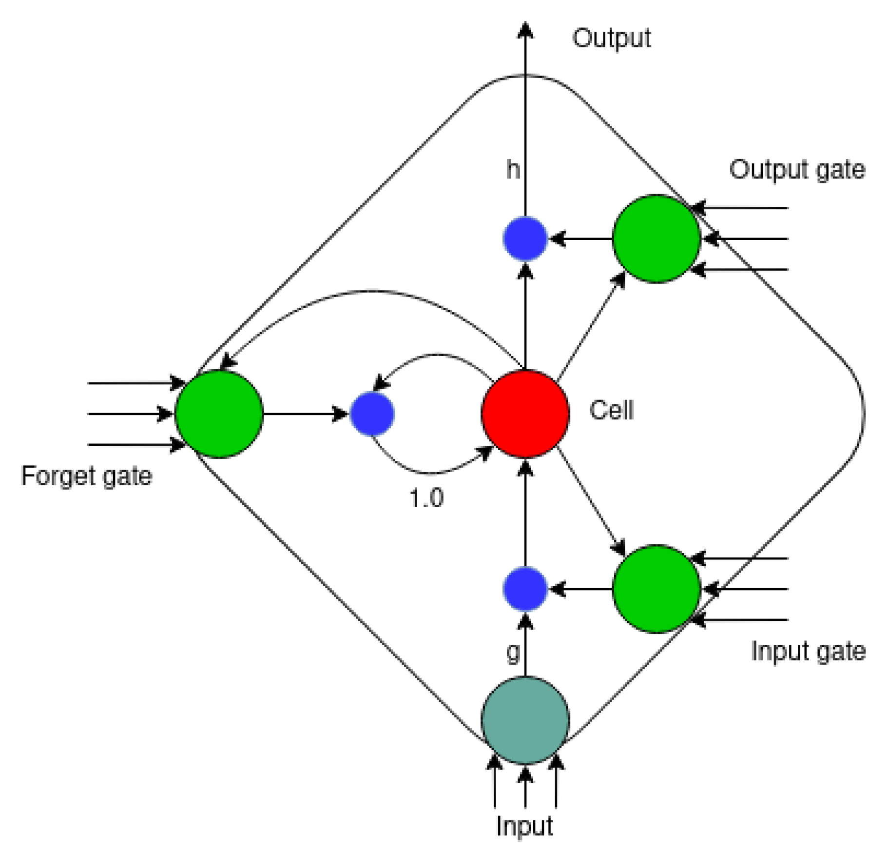
The architecture of a long short-term memory (LSTM) network is defined by memory blocks, where each block has one or more interconnected memory cells and three multiplicative units. The three multiplicative units are input, output, and forget gates. These gates can be understood as write, read, and reset operations, respectively [19]. Figure 2 shows a memory block of an LSTM network, and Figure 1c shows a schematic of an LSTM architecture.

Figure 2. A memory block with a cell. The inner state is held with a connection of fixed weight 1. The three gates collect activation from inside and outside the block and control the cell through the multiplicative units, represented as smaller blue circles. The input and output activation functions of the cell are represented as h and g. Source: adapted from [19].

When the input unit remains closed for an extended period, this cell will not be activated by new inputs into the network, thus, retaining the information in the network for longer. LSTM networks can also be implemented in a bidirectional architecture. Bidirectional LSTM networks ensure that most of the input sequence is preserved.

2.8. Generative Adversarial Network

As described by [20], a generative adversarial network (GAN) can be described as a game between two networks, where one network is the generator (G) and the other is the discriminator (D). The generator creates samples derived from the training data. Using traditional methods of supervised learning for classification, the discriminator evaluates whether the generated samples are real or fake, according to the training data.

Both networks are defined as functions. G is defined as a $G(z;{\theta }^{(G)})$, where z is the input vector and ${\theta }^{(G)}$ is a set of learnable parameters (for example, weights), and D is defined as $D(x;{\theta }^{(D)})$, where x is the input (whether x is real or generated by G) and ${\theta }^{(D)}$ is a set of parameters.

Both the G and D networks have cost functions defined, respectively, as follows:

$$\begin{array}{c}\hfill J^{(G)}({\theta }^{(D)},{\theta }^{(G)})\end{array}\mathrm{and}\begin{array}{c}\hfill J^{(D)}({\theta }^{(D)},{\theta }^{(G)}).\end{array}$$

(5)

The primary objective of both networks is to minimize their cost functions. G attempts to accomplish the objective by adjusting ${\theta }^{(G)}$ although it does not have control over ${\theta }^{(D)}$, and vice versa for D. Therefore, the solution of this game is to find the tuple $({\theta }^{(G)},{\theta }^{(D)})$, where ${\theta }^{(G)}$ is the local minimum of $J^G$ and ${\theta }^{(D)}$ is the local minimum of $J^D$ [16]. Figure 1d shows a schematic of a GAN architecture.

Figure 3. Architecture of a temporal block and the TCN. Source: adapted from [21].

3. Related Work

In the previous section, we discussed some Deep Learning architectures and their methods of operation. With this knowledge, our objective is to test these DL implementations. Therefore we will use implementations applied to seismic inversion based on published studies, to assess how they perform in a test environment. This section describes the sources and the studies that serve as the practical basis for this paper.

3.1. Acoustic Impedance Inversion Using a Temporal Convolutional Network

In [21], the authors proposed a TCN model for the acoustic impedance inversion. Their goal with this architecture was to use a network that can be trained well on a limited amount of training data. Although CNNs can find local trends compared to the input sequence, they can only find long-term dependencies when more layers are added, thus creating a need for more parameters. Hence, they are impracticable to train with a limited amount of data.

The TCN implementation was based on a series of temporal blocks. Figure 3a shows the structure of a temporal block. As mentioned in Section 2.6, TCNs make use of dilated convolutions, which allows them to have a large receptive field, thus allowing the network to look for large portions of the input without the need for deeper layers. The architecture used to obtain seismic inversions is shown in Figure 3b. The concatenation at the end was introduced to compensate for the losses of high-frequency information after many successive convolutions.

3.2. Convolutional Neural Network for Seismic Impedance Inversion

In [10], a 1D convolutional neural network (CNN) is used to train synthetic seismograms and, from these, predict impedance traces. The architecture of the network is defined with two convolutional layers, where each layer contains a 1D convolutional kernel with a size of 300 samples (proportional to the wavelet size), a stride of 1 sample, and a ReLU layer at the end. The first layer has 60 convolutional neurons, and the second layer has one convolutional neuron. Figure 4 shows the architecture defined by the authors.

Figure 4. A 1D CNN architecture. Source: adapted from [10].

To make the implementation more robust, the authors tested the network by predicting impedances, where the synthetic seismograms were based on several rock-model configurations. These seismograms were created using Kennett reflectivity and the data augmentation method. For training, they utilized 2000 seismic traces, where 70% of these were for training and the remaining 30% were split in half for validation and testing. The correlation of the results obtained by the CNN was 95% (using an unspecified metric), compared with 89% from a model-based least-squares inversion. Lastly, a seismic inversion was performed on the Volve dataset, which contains 1300 impedance traces. A total of 750 traces were used for training, while the 550 remaining traces were split in half for validation and testing. The metric used for validation was the Pearson correlation coefficient (PCC).

3.3. Seismic Impedance Inversion Using Generative Adversarial Network

In [22], the authors used a GAN network using semi-supervised methods for seismic inversion. The network comprises three key components: the generator G, the discriminator D, and a forward model F. The generator G receives a seismic trace x as the input and generates the related acoustic impedance as the output. The discriminator D receives the acoustic impedance as the input and returns a scalar which represents the probability of the acoustic impedance x belonging to the labeled dataset. The forward model F is a convolutional network that learns seismic traces from the impedance. Thus it is the inverse of G. Consequently, F allows training on unlabeled data because, for each seismic trace, it can obtain the error made by G in the inversion process by calculating the difference between $F(G(x))$ and x. This difference tends to zero provided both networks are trained. Both F and G have the same architecture, as shown in Figure 5.

Figure 5. Architecture of a residual block and the generator. Source: adapted from [22].

This implementation aims to take advantage of a WGAN-GP (Wasserstein GAN+gradient penalty) in a cGAN (conditional GAN). Using a cGAN guarantees that the network learns to map each seismic trace to the respective impedance, making the input seismic data conditional on the impedance prediction. This way, the WGAN-GP is an improvement over the WGAN, which in turn has performance and stability advantages compared with a regular GAN.

To show the efficiency of the GAN, the authors performed three experiments applied to public data. The first one used the Marmousi2 dataset and compared the results with a conventional CNN with the same architecture defined in the forward model. The second used the SEAM dataset and compared the results with other models from other authors, i.e., a joint learning 2D TCN, a 2D TCN, a 1D TCN, and an LSTM. The third experiment used the Volve dataset mentioned earlier and compared the results with the same 1D CNN cited previously.

The Marmousi2 dataset contains 13,601 pair traces (seismic and impedance), and in the first experiment the authors chose 101 evenly-spaced traces for training. Of the 13,500 traces remaining, 10% were randomly selected for validation and 90% for testing. The metrics for validation were the MSE, coefficient of determination $r^2$, and Pearson correlation coefficient (PCC). The Volve dataset used in the third experiment contains 1300 impedance traces, of which 750 traces were randomly chosen as labeled training data, and the 550 traces that remained were randomly split in half (275 traces each) as unlabeled testing data and validation data. In this experiment, a small change was made in the network: all the kernel values were changed from 300 to 80, since the data only had 160 time points. The metric for validation was the PCC.

3.4. Summary

As mentioned in the previous subsections, each experiment used metrics and datasets that were appropriate for their respective experiments. Table 1 gives a summary of each experiment, including what DL model was used and the respective datasets, training data (shown as “traces used/total traces”), metrics, and results.

Table 1. Summary of each experiment described in this section.

DL Model	Datasets	Training Data	Metrics	Results	Source
1D CNN	Synthetic	1400/2000 traces	unspf.	0.95	[10]
	Volve	750/1300 traces	PCC	0.82
GAN	Marmousi2	101/13,601 traces	MSE	0.0184	[22]
			PCC	0.9948
			$r^2$	0.9874
	2D SEAM	34/1719 traces	PCC	0.9902
			$r^2$	0.9753
	Volve	750/1300 traces	PCC	0.88
TCN	Marmousi2	19/2721 traces	PCC	0.96	[21]
			$r^2$	0.91

Table 1. Summary of each experiment described in this section.

DL Model	Datasets	Training Data	Metrics	Results	Source
1D CNN	Synthetic	1400/2000 traces	unspf.	0.95	[10]
	Volve	750/1300 traces	PCC	0.82
GAN	Marmousi2	101/13,601 traces	MSE	0.0184	[22]
			PCC	0.9948
			$r^2$	0.9874
	2D SEAM	34/1719 traces	PCC	0.9902
			$r^2$	0.9753
	Volve	750/1300 traces	PCC	0.88
TCN	Marmousi2	19/2721 traces	PCC	0.96	[21]
			$r^2$	0.91

4. Methodology

As mentioned in Section 3, we can see that each DL implementation utilizes different datasets and metrics to validate its performance. However, it is not sufficient just to observe which one is used, since we cannot compare them, because each one utilizes different datasets or different training data. This section show the experiments on these DL implementations and how the networks perform when they are applied over the same datasets and trained with the same training data.

We applied all the networks on two datasets and measured their performances using quantitative and qualitative analyses. The datasets used in this experiment were Marmousi2 [23] and Volve. The former is based on the North Quenguela trough geology, in Kwanza Basin, Angola. The latter is a well location based on the open-source implementation provided by [10].

The following subsections cover the dataset used in the experiments, the metrics, and the model description for each Deep Learning method used.

4.1. Datasets

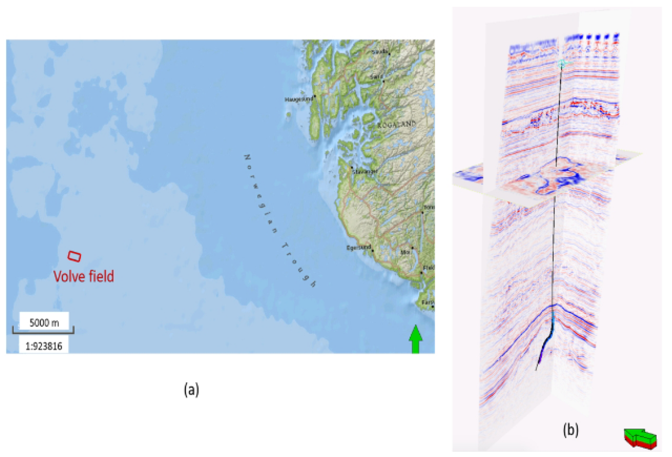
Two datasets were chosen for the experiments. The first was the Volve dataset from the location shown in Figure 6a, where 1300 impedance traces were generated from the statistics of the impedance log from the well location shown in Figure 6b using the data augmentation method as described in [10]. In every experiment listed here, of 1300 traces, 750 were used for training, and the remaining 550 traces were split in half for validation and testing. The results presented here are the three impedance traces resulting from the prediction of the network in the testing set.

The second dataset is the Marmousi2 dataset, which as the name implies is an extension of the original Marmousi dataset. Marmousi2 is 17,000 m long and 3500 m deep, with different geological structures such as gas channels, petroleum channels, geological faults, and materials such as sand, salt, and shale. Furthermore, Marmousi2 represents an exploration scenario in deep water, which is very common in petroleum exploration [23]. This dataset was chosen because it is one of the most frequently utilized public datasets for seismic inversion benchmarking.

Marmousi2 has 13,601 pair traces, where 2800 are seismic trace samples and 2801 are seismic impedance traces. Two important points to note regarding Marmousi2 are the two gas reservoirs, one in the upper-left corner and the other in the lower central region. The former region is more visible because it is a low-impedance acoustic region, while the latter is less visible as only the impedance is considered. Both regions can be seen in Figure 7, described as “Gas-charged sand channel” and “Gas and oil cap”, respectively. Identifying these regions is important for measuring the quality of a seismic inversion because it is the main objective of the inversion in this context.

It is important to note that the objective of a seismic inversion is not to identify the rock material, i.e., to identify the existence of petroleum or gas, but to identify whether rock structures exist with conditions suitable for storing such substances. Figure 7 shows petroleum regions in green and gas regions in red.

As mentioned previously, this dataset contains 13,601 pair traces, and we selected 101 evenly-spaced traces for training. Of the 13,500 traces remaining, 10% were randomly selected for validation and 90% for testing. The results presented are three impedance traces resulting from the prediction by the network from the testing set, in addition to an image generated from the inversion of the whole set for a visual comparison.

Figure 6. (a) Volve field highlighted on a map of the offshore North Sea. (b) Seismic data highlighting a well trajectory from the Volve field. Source: extracted from [10].

Figure 7. Detail of structures from Marmousi2 dataset. Source: extracted from [23].

4.2. Metrics

In Section 4.1, we discussed the datasets and how the data were used for the quantitative analysis. In this subsection, we discuss the metrics for the qualitative analysis. The metrics chosen for the experiments were the mean squared error (MSE) and the structural similarity index measure (SSIM). The former metric is proportional to the data scale and requires knowledge of the data in order to measure the quality of the results.

The latter, proposed by [24], was chosen to compare the images generated by the inversion. This is essential because, in subsurface exploration, it is more interesting to have a global comprehension of the subsurface (provided by the image) than only pieces of information about acoustic impedance values in specific regions. Thus, it is important to measure the quality of the generated image.

The SSIM is an index between 0 and 1, where 0 represents no similarity and 1 represents absolute similarity. This means that this metric does not depend on the data scale and is not affected by data normalization, which is usually applied in training. Equation (6) shows the SSIM function:

$$SSIM(x,y)=\frac{(2{\mu }_x{\mu }_y+c_1)(2{\sigma }_{xy}+c_2)}{({\mu }_x^2+{\mu }_y^2+c_1)({\sigma }_x^2+{\sigma }_y^2+c_2),}$$

(6)

where x and y are the original and predicted images, respectively, $\mu$ is the mean from the respective image, ${\sigma }^2$ is the variance from the respective image, ${\sigma }_{xy}$ is the covariance of x and y, and $c_1$ and $c_2$ are variables to stabilize the division.

4.3. Implementation

Five DL implementations were used for the experiments: LSTM, GAN, two 1D CNNs, and TCN. Section 2 describes the architectures for each network and Section 3 describes the motivation for, and experiments realized with, each network. Both the CNN [10] and TCN [21] were tested using the sources provided by the authors. However, we re-implemented the network described in [22] in TensorFlow, based on the information provided in the paper. To distinguish the 1D CNNs, we refer to the CNN in [10] as D_CNN and the other one, in [22], as G_CNN.

The LSTM network is our implementation, to be compared with the others and to show how this network performs on the selected datasets. The implementation was performed in TensorFlow, and the network has seven layers, where each layer can be described as follows:

• Bidirectional LSTM, with 120 neurons and return sequences defined as True;
• Batch normalization, $ϵ=0.0001$;
• ReLU;
• A dense network layer with 150 neurons;
• A dense network layer with 50 neurons;
• Bidirectional LSTM, with 150 neurons and return sequences defined as True;
• A dense network layer with one neuron.

For any parameter not specified, it was assumed that default values were used.

5. Experimental Results

In this section, we show the results of the experiments divided into three subsections. Each subsection represents a test environment divided into three categories: prediction of impedances from seismic traces from a well trajectory and prediction of impedances from a noisy geological structure and a non-noisy geological structure. The dataset chosen for the former was Volve, while that for the latter was Marmousi2.

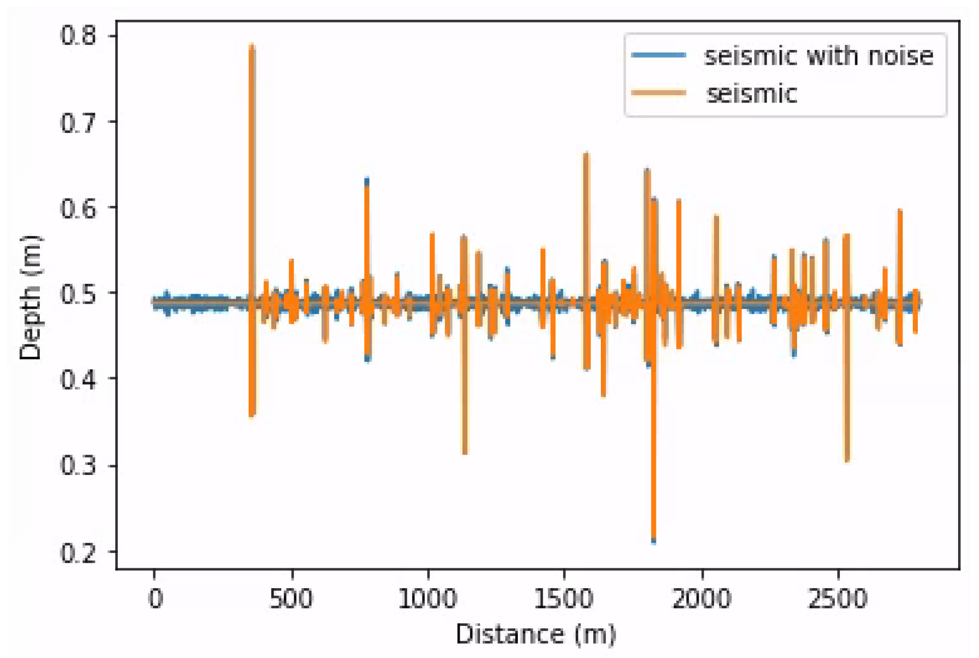
As described in the last subsection, we added noise with spatial correlation to simulate real noise. We generated white noise, sampled it from a normal distribution, and convoluted it with the same wavelet used to generate the seismic data. Then, we defined a variance and added it to the seismic trace. This operation was applied to training, validation, and testing data. Equation (7) shows the process of adding noise to an acoustic seismic trace:

$$N=\left(\frac{p(|S|)\ast W}{\sigma (p(\left|S\right|)\ast W)}\times \frac{\sigma (S)}{\sqrt{r}}\right)+S$$

(7)

where N is the resulting acoustic seismic trace with noise, S is the acoustic seismic trace, W is the wavelet, ∗ is the convolution operation, $\sigma$ is the standard deviation, and r is a noise rate constant.

Figure 8 shows the results, comparing an acoustic seismic trace with and without noise.

Figure 8. Two acoustic seismic traces, one with noise and the other without, stacked together.

5.1. Volve Dataset

We compiled the LSTM network using Adam optimization, setting the learning rate to 0.001 and MSE as the loss function. For training, we defined 500 epochs, a batch size of 5, and early stopping as a callback (a function to be called in each epoch), which stops the training if there is no improvement in the training loss. For the parameters of the callback function, we defined mode as the minimum value that stops the process if training losses keep increasing, the number of epochs to be monitored before the decision to stop the training as 300, and True as the utilization of restore_best_weights, which returns the weights from the best epoch monitored, i.e., with the smallest training loss obtained. Figure 9a shows five prediction examples of the network using the Volve dataset.

Figure 9. Prediction results for three seismic trace tests from the Volve dataset.

We compiled the GAN network using Adam optimization and set the learning rate to 0.001. The training loss function was implemented as described by [22]. We trained with batch sizes of 75 and 2000 epochs. During the training, the discriminator was trained for five steps, and then in the next step, the generator was trained. Figure 9d shows three examples for this experiment.

We compiled the G_CNN network using Adam optimization and set the learning rate to 0.001. The training loss function was the MSE, the batch size was 75, and we trained for 2000 epochs. Figure 9e shows three examples for this experiment. Table 2 shows the metric results.

Table 2. Results of the experiments on the Volve dataset with the five neural network models. The metrics were obtained by comparing the test data and the result generated by each network. The symbol ↓ indicates that the smaller the value, the better the result, while ↑ indicates that the bigger the value, the better the result.

Dataset	Metric	LSTM	TCN	D_CNN	GAN	G_CNN
Volve	MSE ↓	$0.0044$	$0.0286$	$0.0236$	$0.8165$	$0.9240$
	SSIM ↑	$0.9661$	$0.7301$	$0.7132$	$0.8542$	$0.0055$

5.2. Marmousi2 without Noisy Seismic Data

The configuration of the LSTM network was mostly the same as that shown in Section 4.3, with the exception that in this experiment, we defined 300 neurons in both LSTM layers. The compilation settings in this experiment were the same as those given in Section 5.1. Figure 10a shows three impedance prediction examples and Figure 11a shows the prediction and the original section of the impedance side by side.

Figure 10. Prediction results for three seismic trace tests from the Marmousi2 dataset (without noisy data).

Figure 11. Prediction results for impedance sections for testing from the Marmousi2 dataset (without noisy data).

For the D_CNN network, Figure 10c shows three examples of the experiment, and Figure 11c shows the prediction and the original section of the impedance side by side.

For the TCN network, Figure 10b shows three examples of the experiment, and Figure 11b shows the prediction and the original section of the impedance side by side.

The configuration of the GAN network was mostly the same as that shown in Section 3.3, with the exception that in this experiment, we defined the batch size as 10, as the authors also did. The compilation settings in this experiment were the same as those shown in Section 5.1. Figure 10d shows three impedance prediction examples, and Figure 11d shows the prediction and the original section of the impedance side by side.

We compiled the G_CNN network using Adam optimization and set the learning rate to 0.001. The training loss function was the MSE, the batch size was 10, and we trained for 2000 epochs. Figure 10e shows three examples of the experiment, and Figure 11e shows the prediction and the original section of the impedance side by side. Table 3 shows the metric results.

Table 3. Results of the experiments on the Marmousi2 dataset without noisy seismic data with the three neural network models. The metrics were obtained by comparing the test data and the result generated by each network. The symbol ↓ indicates that the smaller the value, the better the result, while ↑ indicates that the bigger the value, the better the result.

Dataset	Metric	LSTM	TCN	D_CNN	GAN	G_CNN
Marmousi2 (without noisy seismic data)	MSE ↓	$0.1143$	$0.3024$	$1.5737$	$0.0026$	$0.0036$
	SSIM ↑	$0.6122$	$0.8019$	$0.6857$	$0.7876$	$0.7614$

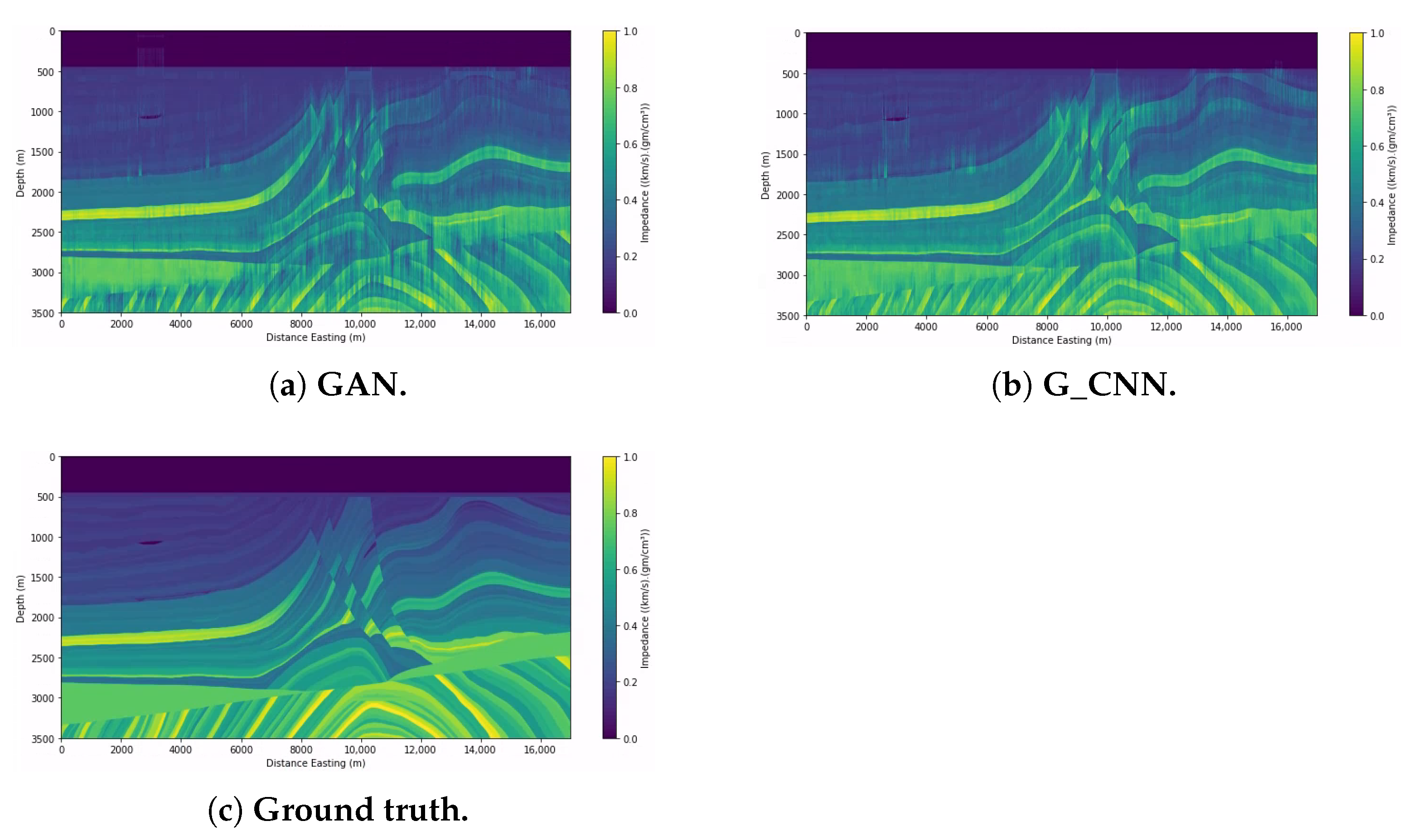
5.3. Marmousi2 Dataset with Noisy Seismic Data

The configuration and compilation of the GAN network were the same as described in the previous subsection. Figure 12a shows three impedance prediction examples, and Figure 13a shows the prediction and the original section of the impedance side by side.

Figure 12. Prediction results for three seismic trace tests from the Marmousi2 dataset (with noisy data).

Figure 13. Prediction results for impedance sections for testing from the Marmousi2 dataset (with noisy data).

We compiled the G_CNN network in the same way as shown in the previous subsection. Figure 12b shows three examples of the experiment, and Figure 13b shows the prediction and the original section of the impedance side by side. Table 4 shows the metric results.

Table 4. Results of the experiments on the Marmousi2 dataset with noisy seismic data with the two neural network models. The metrics were obtained by comparing the test data and the result generated by each network. The symbol ↓ indicates that the smaller the value, the better the result, while ↑ indicates that the bigger the value, the better the result.

Dataset	Metric	GAN	G_CNN
Marmousi2 (noisy seismic data)	MSE ↓	$0.0068$	$0.0058$
	SSIM ↑	$0.5960$	$0.5712$

6. Discussion

In this section, we discuss the results of the experiments described in the previous section. Each subsection corresponds to the respective test environment.

6.1. Volve Dataset

As can be seen from the images presented in the previous subsections, each network predicts differently for each seismic trace. On the Volve dataset, LSTM seems to perform better on all three, and the qualitative analysis presented in Table 2 leads to the same conclusion, with LSTM performing better for both metrics listed. The superiority of LSTM could be explained by the use of bidirectional layers, which provides the advantage of registering more data information for more extended periods, thus ensuring that the learning method retains more information.

Comparing G_CNN with GAN, we can see that the latter performed better, and the results in Table 2 tend to agree. A similar experiment with both a 1D CNN and a GAN was presented in Section 3.3, and again, GAN performed better. We can see that the results favor the GAN in this case due to the use of unlabeled data in training.

The results obtained by the TCN and by the D_CNN were very similar, which is surprising considering the much higher complexity of the TCN architecture, showing that highly complex architectures may be useful only for the specific dataset they were built to learn.

6.2. Marmousi2 Dataset (without Noisy Seismic Data)

We can see that LSTM was the worst-performing network in this experiment, and the metrics in Table 3 confirm that even though the network had more units in its bidirectional layers, this was not enough to enable it to perform better. Figure 10a shows that the prediction for some selected traces was extremely poor, with little to no correlation between the predicted and the expected acoustic impedances. Since it is a little more unstable in its predictions, Figure 11a shows that the LSTM network could only replicate some interfaces, and the gas channel in the upper-left corner is barely visible.

On the other hand, Figure 11c shows that D_CNN performed much better in generating the image, although it was very noisy. We can see one of the gas channels, but only with considerable surrounding noise. The visual comparison between some selected traces, shown in Figure 10c, shows that the correlation between expected and predicted traces was not satisfactory.

Figure 11b shows that the TCN was the best-performing network, because its several convolutional layers in each temporal block (therefore, its greater number of neurons) allowed better generalization. Despite the excellent result, there is a noticeable generalization difficulty in the deeper sections where the layer variation is more significant. This difficulty could be caused by the use of several dilated convolution layers with a dilated core because, given that these layers calculate the output based on a large portion of the input, the network performance may be reduced in the part where the layer variation is more visible and the layers are slimmer, which would require a local prediction. Figure 10b shows a good correlation between predicted and expected acoustic seismic traces.

Figure 11d,e show that both GAN and G_CNN gave satisfactory results, though GAN performed slightly better than G_CNN. Both networks performed better than LSTM and D_CNN, due to the use of unlabeled data by GAN and the use of residual blocks by G_CNN, guaranteeing that the seismic inputs condition the impedance outputs.

6.3. Marmousi2 Dataset (with Noisy Seismic Data)

We can see that both networks had similar good results, though Table 4 shows that GAN performed slightly better. In Figure 13a,b, we can see that both networks detected the gas sand channel in the upper-left corner well, although with noise present, GAN could predict some gas sands in the center, particularly on the upper right (see Figure 7 for reference). We can also see that GAN could predict some of the faults better, unlike CNN, with noticeable noise around the fault.

Comparing the trace predictions in Figure 12a,b we can again see the superiority of the GAN in the three traces selected, although both networks performed poorly on trace 7003, since from this trace and above, the interfaces between structures tended to be more accentuated. Both networks utilized convolutional layers for their predictions, but GAN performed better due to the use of unlabeled data for training.

7. Conclusions

In this work, we compared different Deep Learning implementations performed under the same conditions, where these conditions were as close as possible to a real environment. We observed how the selected DL methods performed in our three test environments. Utilizing both qualitative and quantitative analyses, we observed how they performed compared with each other, thus producing methods that allow simple comparisons between different DL models.

From these experiments, we noted that each DL model has advantages and disadvantages in each test environment, showing that they are equally crucial, with specific abilities that help solve different seismic impedance inversion problems. In our first environment, the prediction of seismic impedances from seismic traces from a well trajectory, LSTM showed the best results, due to its bidirectional layers, which helped register information for extended periods. However, the other networks tested had sufficiently satisfactory results. In the second environment, the prediction of impedances from a geological structure, TCN showed the best results, due to its convolutional layers, while LSTM obtained no acceptable results. Both G_CNN and GAN showed satisfactory results, and D_CNN showed acceptable results with noise. In the third environment, the same as the previous one but with added noise, GAN showed its superiority against the 1D CNN, due to the use of unlabeled data in training, which enabled the best predictions.

Future studies could perform more experiments with noisy seismic data, as in this case where LSTM, TCN, and D_CNN were used to predict seismic impedances from Marmousi2. In addition, more similar experiments with other DL implementations could be performed in even more realistic circumstances, for example, with fewer seismic traces for training, since 101 traces is still a relatively high number for training data. Another possibility is the use of semi-supervised methods, which are promising contenders for optimum performance because they can take advantage of unlabeled data. This analysis would assist in determining what DL architecture is best for real problems.

References

- Chen, Y.; Chen, H.; Xiang, K.; Chen, X. Geological structure guided well log interpolation for high-fidelity full waveform inversion. Geophys. J. Int. 2016, 207, 1313–1331. [Google Scholar] [CrossRef]
- de Souza, M.G. Inversão Sísmica Acústica Determinística Utilizando Redes Neurais Artificiais. Master’s Thesis, Pontífica Universidade Católica do Rio de Janeiro, Rio de Janeiro, Brazil, 2018. [Google Scholar]
- Mosser, L.; Dubrule, O.; Blunt, M.J. Stochastic seismic waveform inversion using generative adversarial networks as a geological prior. arXiv 2018, arXiv:1806.03720. [Google Scholar]
- Cooke, D.; Cant, J. Model-Based Seismic Inversion: Comparing Deterministic and Probabilistic Approaches. 2010. Library Catalog. Available online: Csegrecorder.com (accessed on 6 April 2020).
- Robinson, G. Stochastic Seismic Inversion Applied to Reservoir Characterization. 2001. Library Catalog. Available online: Csegrecorder.com (accessed on 6 April 2020).
- Russel, B.H. Introduction to Seismic Inversion Methods; Society of Exploration Geophysicists: Tulsa, OK, USA, 1988; p. 178. [Google Scholar]
- Dramsch, J.S. 70 years of machine learning in geoscience in review. arXiv 2020, arXiv:2006.13311. [Google Scholar]
- Laloy, E.; Hérault, R.; Jacques, D.; Linde, N. Training-image based geostatistical inversion using a spatial generative adversarial neural network. Water Resour. Res. 2018, 54, 381–406. [Google Scholar] [CrossRef]
- Laloy, E.; Hérault, R.; Lee, J.; Jacques, D.; Linde, N. Inversion using a new low-dimensional representation of complex binary geological media based on a deep neural network. Adv. Water Resour. 2017, 110, 387–405. [Google Scholar] [CrossRef]
- Das, V.; Pollack, A.; Wollner, U.; Mukerji, T. Convolutional neural network for seismic impedance inversion. Geophysics 2019, 84, R869–R880. [Google Scholar] [CrossRef]
- Mavko, G.; Mukerji, T.; Dvorkin, J. The Rock Physics Handbook: Tools for Seismic Analysis of Porous Media, 2nd ed.; Cambridge University Press: Cambridge, UK, 2009. [Google Scholar] [CrossRef]
- Oldenburg, D.W.; Scheuer, T.; Levy, S. Recovery of the acoustic impedance from reflection seismograms. Geophysics 1983, 48, 1305–1414. [Google Scholar] [CrossRef]
- Salleh, M.S.; Ronghe, S. Reservoir Characterization on Thin Sands in South West Ampa 21 Area (BLK11) Using Seismic Inversion; SEG Techinical Program Expanded Abstracts; Society of Exploration Geophysicists: Tulsa, OK, USA, 1999; pp. 1568–1573. [Google Scholar]
- Sancevero, S.S.; Remacre, A.Z.; de Souza Portugal, R. O papel da inversão para a impedância acústica no processo de caracterização sísmica de reservatórios. Rev. Bras. GeofíSica 2006, 24, 495–512. [Google Scholar] [CrossRef]
- Debeye, H.W.J.; Van Riel, P. Lp-Norm Deconvolution. Geophys. Prospect. 1990, 38, 381–403. [Google Scholar] [CrossRef]
- Goodfellow, I.; Bengio, Y.; Courville, A. Deep Learning; Adaptive Computation and Machine Learning; The MIT Press: Cambridge, MA, USA, 2016. [Google Scholar]
- Albawi, S.; Mohammed, T.A.; Al-Zawi, S. Understanding of a convolutional neural network. In Proceedings of the 2017 International Conference on Engineering and Technology (ICET), Antalya, Turkey, 21–23 August 2017; pp. 1–6. [Google Scholar] [CrossRef]
- Lea, C.; Vidal, R.; Reiter, A.; Hager, G.D. Temporal Convolutional Networks: A Unified Approach to Action Segmentation. In Computer Vision—ECCV 2016 Workshops; Hua, G., Jégou, H., Eds.; Springer International Publishing: Cham, Switzerland, 2016; pp. 47–54. [Google Scholar]
- Graves, A. Supervised Sequence Labelling with Recurrent Neural Networks, 1st ed.; Springer: Berlin/Heidelberg, Germany, 2012. [Google Scholar] [CrossRef]
- Goodfellow, I.; Pouget-Abadie, J.; Mirza, M.; Xu, B.; Warde-Farley, D.; Ozair, S.; Courville, A.; Bengio, Y. Generative Adversarial Networks. Commun. ACM 2020, 63, 139–144. [Google Scholar] [CrossRef]
- Mustafa, A.; AlRegib, G. Estimation of Acoustic Impedance from Seismic Data using Temporal Convolutional Network. In SEG Technical Program Expanded Abstracts 2019; Society of Exploration Geophysicists: Tulsa, OK, USA, 2019; pp. 2554–2558. [Google Scholar]
- Wu, B.; Meng, D.; Zhao, H. Semi-Supervised Learning for Seismic Impedance Inversion Using Generative Adversarial Networks. Remote Sens. 2021, 13, 909. [Google Scholar] [CrossRef]
- Martin, G.S.; Wiley, R.; Marfurt, K.J. Marmousi2: An elastic upgrade for Marmousi. Lead. Edge 2006, 25, 156–166. [Google Scholar] [CrossRef]
- Wang, Z.; Bovik, A.; Sheikh, H.; Simoncelli, E. Image quality assessment: From error visibility to structural similarity. IEEE Trans. Image Process. 2004, 13, 600–612. [Google Scholar] [CrossRef] [PubMed]