2.3. Real-Time Engine Model
The engine is modelled using a zero-dimensional (0D) mean value approach [
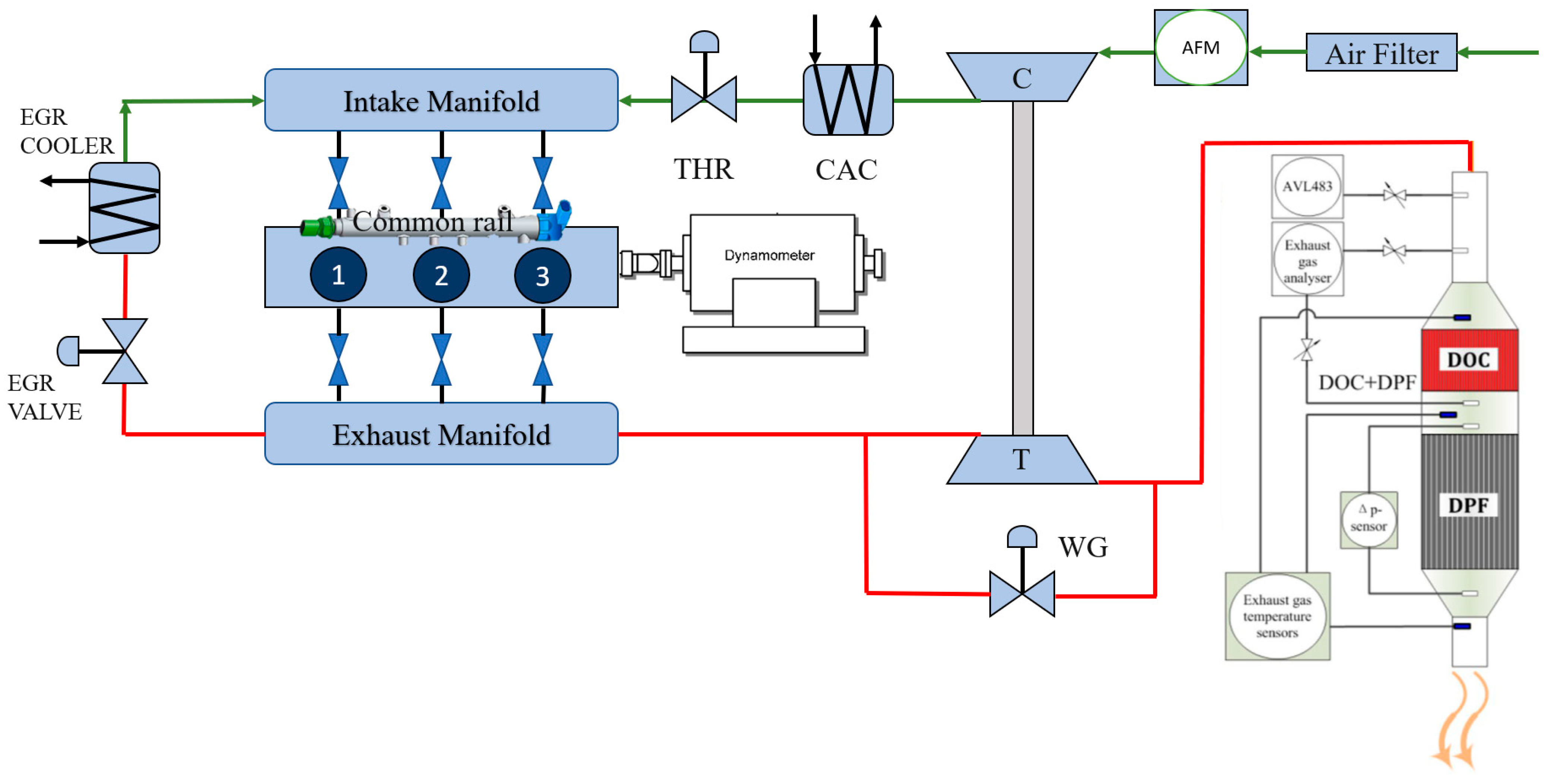
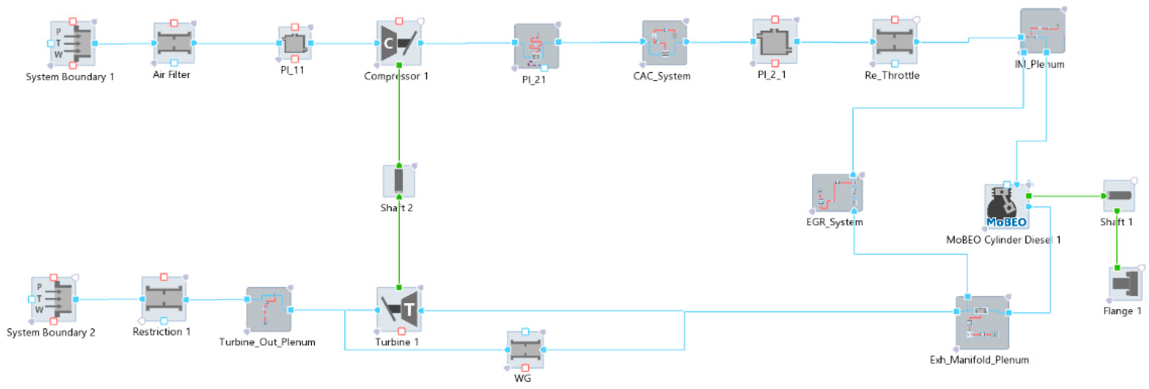
37] within the commercially available software AVL CRUISE M™ with MoBEO (model-based engine optimization) libraries, which integrates physical and empirical models (
Figure 4): the airpath of the modeled ICE was totally physical, while the cylinder model was based on a semi-physical modeling approach. MoBEO allows concept model capability instead of complex cylinder configurations: the in-cylinder processes are tuned using fit parameters based on a huge amount of engine test bed data. Then, MoBEO demands basic cylinder and fueling parameters coming from the test bench to perform the combustion refinement based on previously embedded measurements. An additional part of this semi-physical approach is made of the engine-out emission models.
Therefore, in order to take into account the effect of different engine calibration parameters such as rail pressure, Start of Injection (SOI), pilot injection, EGR rates and operating conditions on combustion, MoBEO combustion libraries were applied. The MoBEO model divides the in-cylinder content into three thermodynamic zones, each with its own composition and temperature. The main unburned zone is made of all trapped mass at intake valve closure. The spray is separated into two main parts, i.e., burned and unburned zones. The former contains the product of the combustion process, and the latter includes the fuel and entrained gas. The model considers fuel evaporation, mixing, and burning process. The sub-model defining the combustion contains three calibration multipliers:
Pressure at start of injection correction (PSOIC).
Combustion delay correction (CDC).
MFB (mass fraction burned) 50% correction (MFBC).
The following measurements were carried out at Engine Test Bed (ETB) to find the optimum calibration parameters to minimize the Root Mean Squared (RMS) error between experimental and simulated combustion results:
One engine map using only main injection and without Exhaust Gas Recirculation (EGR) to better estimate the injection delay and engine volumetric efficiency.
One engine map with standard calibration for overall model parametrization.
Optimized values of the above calibration parameters (PSOIC, CDC, MFBC) are revealed in
Table 4.
The NOx calculation is based on the extended Zeldovich mechanism, and it is embedded in the MoBEO cylinder code. Two calibration parameters are used to tune the NOx emissions:
NO
x emission multiplier (NEM) → NO
x emissions are scaled by the factor specified in
Table 5NO
x heat-up correction (NHC) → NO
x emissions are scaled by the factor specified in
Table 5, depending on the engine coolant temperature
The second step for calibrating the engine model is to parametrize the restrictions and the plenums. Restrictions are transfer components and they have been modelled using basically orifice equations [
28] considering a nominal reference area (A
ref) and parametrizing the flow coefficient (FC) with test bed data; mass flow (
) depends on the conditions upstream the restriction (temperature T
in and pressure p
in) and pressure downstream the restriction (p
out):
In Equation (1), R
in is the upstream specific gas constant. β is a flow function depending on the gas specific heat ratio (k) and on the pressure ratio (p
out/p
in) across the restriction and it changes for subsonic or sonic flow conditions as:
for subsonic flow and:
for sonic flow.
In similar manner, the velocity in the orifice (u
or) is evaluated as:
where “v” is obtained by Equation (5):
for subsonic flow and by:
for sonic flow.
The dependency of the flow coefficient on the pressure ratio or mass flow throughout the resistive component itself is generally parametrized knowing both the mass flow rate at different stationary engine points and the condition upstream and downstream the restriction.
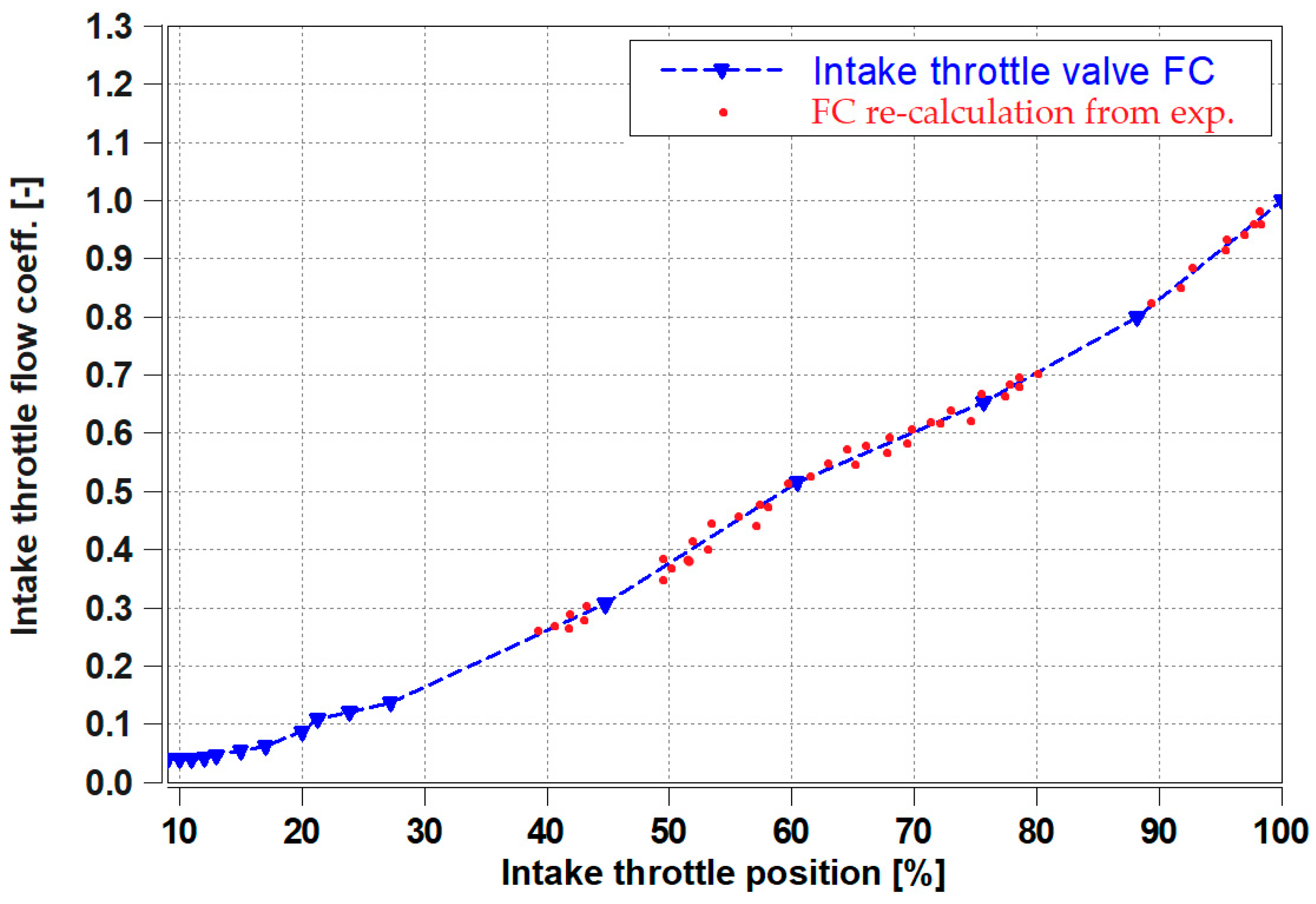
Elements with a variable flow area (for example intake throttle valve and EGR valve) were modeled as restrictions as well, with a fixed nominal area (equal to the maximum nominal area) and a flow coefficient function of the valve opening angle.
Figure 5 shows the flow coefficient parametrized on measured data and used for the intake throttle valve in the engine model. The blue curve represents the flow coefficient used to parametrize the intake throttle valve pressure drop. On the other hand, the red points in the chart represent the punctual values of the flow coefficient, recalculated in each stationary engine operating point. Furthermore, the blue curve has been extended to lower and higher values of the throttle valve opening percentage than those available experimentally, to avoid numerical instabilities during simulations.
A plenum, instead, is a volume component that contains gas. During the engine simulation process, it is filled up and emptied with fresh air or exhaust gases thanks to mass balance equation, energy and species concentration, and state equation calculation. The classic species balance equations [
38] are considered to reproduce the influence of the gas composition on the fluid physical properties for the whole ICE operating map such as different exhaust gas recirculation and different exhaust gas temperatures: this method is necessary to model the states in the storage elements and the flow through the transfer elements. As described in [
39], the classic species approach is useful to reduce the computational cost. Thus, conservation equations for combustion products and fuel vapor are solved. The air mass fraction (µ
air) is linked to the fuel vapor mass fraction (µ
fv), the combustion products mass fraction (µ
cp) and the burned fuel mass fraction (µ
fb) through the following equation:
The air to fuel ratio (AF
CP) is a characteristic quantity that describes the composition and the properties of the combustion products, and it is evaluated by the Equation (8):
The combustion gases composition is calculated from the chemical equilibrium considering dissociation at the high temperatures inside the cylinder. The heat transfer towards the environment was modelled, starting from each plenum, by building a thermal path. This path structure consists of two parts: a convective heat exchange between the solid wall and the gas within the volume, and a convective heat transfer between the environment and the solid wall. The Heat Transfer Coefficient (HTC) between the environment and the solid wall was estimated according to literature values and in particular to [
39], whereas the convective heat transfer (
) between the solid wall and the gas in the plenum, is calculated from the convective law, assuming a constant wall temperature (T
w) and a constant gas temperature (T
gas), according to Equation (9):
where
represents a heat transfer multiplier,
is the heat transfer surface and HTC represents the convective heat transfer coefficient. This latter is evaluated through the Reynolds analogy [
40] and finally tuned acting on the heat transfer multiplier
.
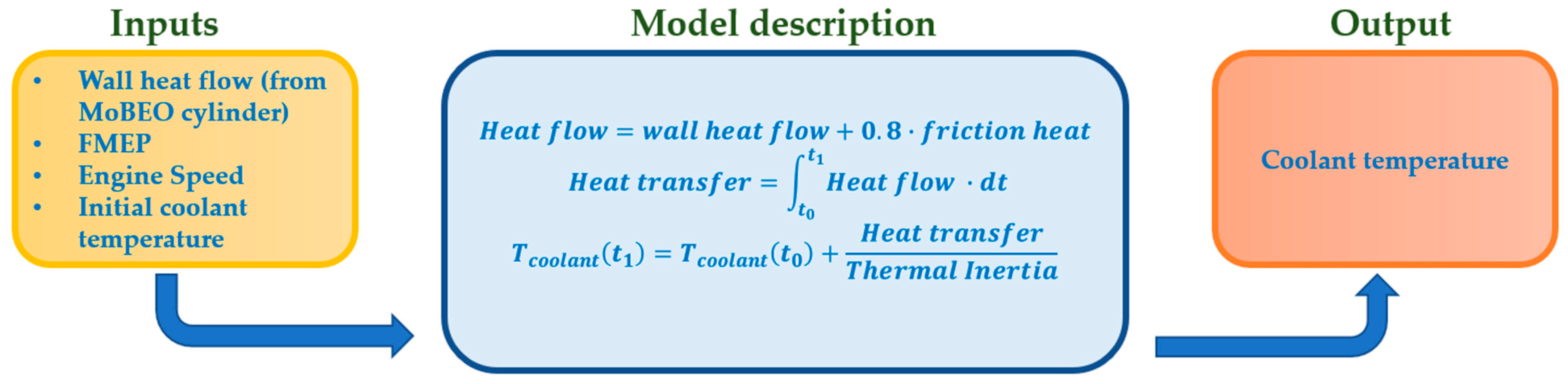
Another important aspect of the engine model is the prediction of the coolant temperature behavior during the warm-up phase because a lot of ECU strategies are based on that temperature. The transient evolution of the coolant temperature is evaluated taking into consideration that in the coolant circuit, the temperature derivative is proportional to the heat flux divided by systems thermal inertia (
Figure 6) [
39]. When the simulated temperature reaches the target thermostat temperature, a saturator signal is activated.
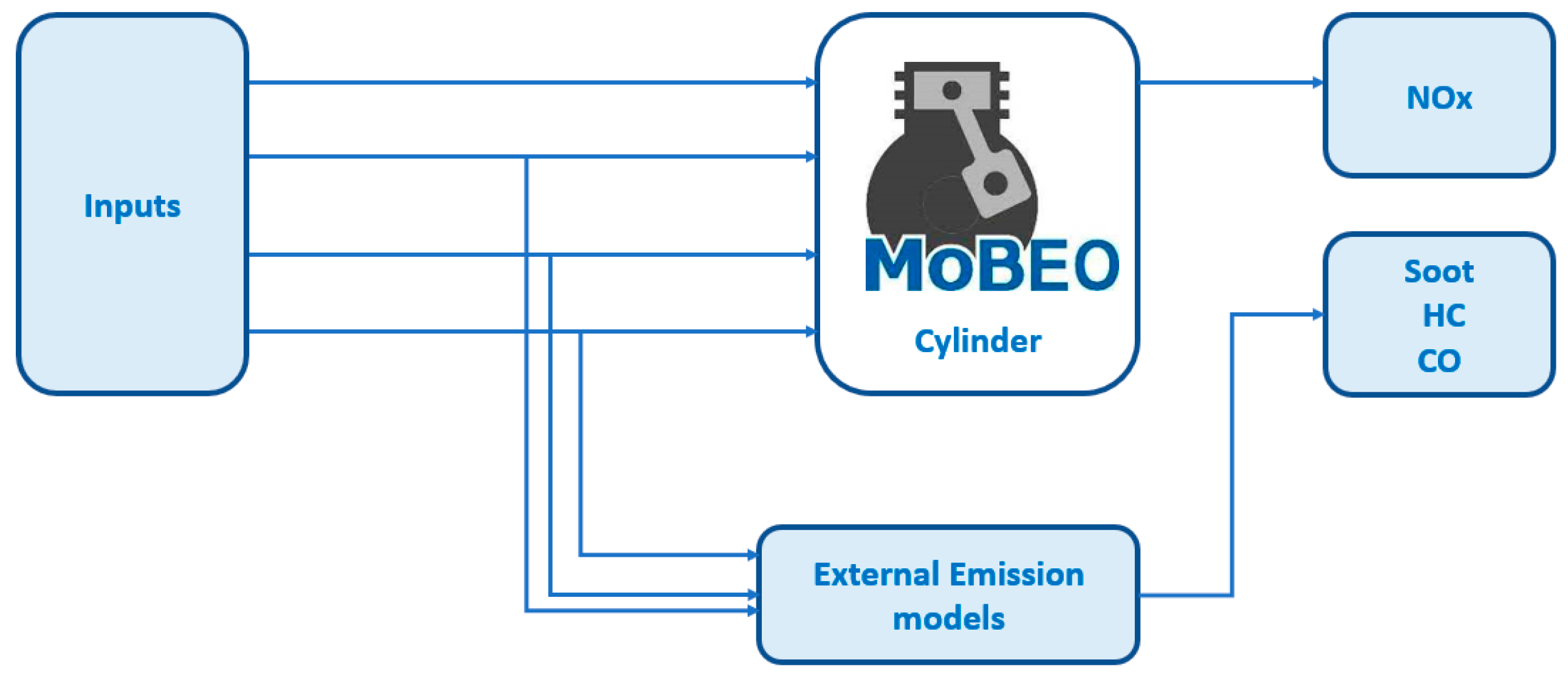
The last step of the ICE model calibration is represented by the engine out emission models. The engine-out nitrogen oxides (NO
x) emissions are estimated by a semi-physical model implemented within the cylinder code and parametrized during the combustion process modelling. For Carbon monoxide (CO), Hydrocarbon (HC) and Soot emissions instead, no such models are present since they are strictly engine dependent. External emission models need to be added to the cylinder block (
Figure 7).
Therefore, a specific design of experiments (DoE) program was delineated to create a user-defined emission models based on empirical correlations. Since the Soot, HC and CO models are built based on measurement data it is necessary to choose physical approach inputs and not measured parameters. In this way, models’ strength in extrapolation areas is guaranteed. For example, the EGR rate is not taken into account as a model input but the oxygen concentration on the intake mass flow to the cylinder is considered. Moreover, it is necessary to keep as few model inputs as possible without compromising the accuracy of the results to ensure real-time calculation.
For this reason, to implement such correlations two ways have been considered: neural networks and polynomials; neural networks promise a very good fit to measure points, they have very weak extrapolation capabilities, and need a very significant calculation effort (frequently not real-time capable) and must be treated as “black box” model unsuitable to being manipulated in order to replicate expected trends. On account of the above shortcomings, polynomial models were chosen instead, and they were generated using an optimization tool. The structure of each user-defined emission models consists of polynomials with terms up to fifth order and includes cross interactions up to fourth order as described in [
39]. The output of these kinds of models is a function of the engine speed, the oxygen content in the cylinder, the rail pressure, the injections timing, the air to fuel ratio and the exhaust mass flow. Dependencies on other engine parameters were ignored since they were deemed less important in agreement with the significance method. An example of used polynomial function considering, for simplicity, only two inputs (x
1, x
2), is shown in Equation (10):
This way, a “grey box” model is obtained, where physical knowledge can be included. The terms within the Equation (10) can be reduced. This means that not all 15 regression coefficients c
0, c
1, …, c
15 will be part of the final model. The model structure graphic in
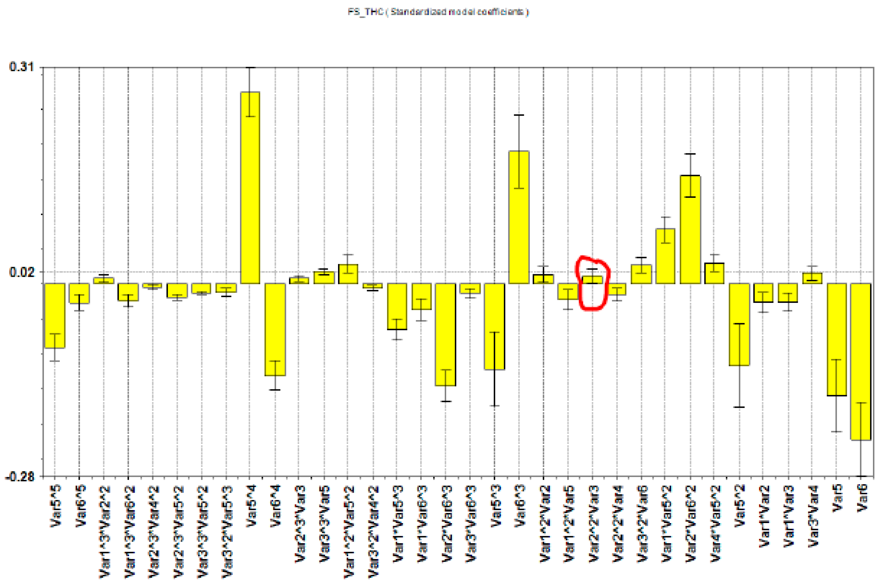
Figure 8 displays standardized HC model coefficients used in the engine model as yellow bars. Error bars of these coefficients describe the 95% confidence intervals. In other words, the graphic displays the influence of each model term on the selected response variable. Terms with a low value but high uncertainty (confidence interval) should be removed to increase the robustness and extrapolation capabilities of the models.
For instance, in
Figure 8, the confidence interval for the term circled in red reaches down to near zero. Thus, the coefficient is not significantly different from zero and therefore does not contribute to the quality of the fit and it might even cause spurious behavior in extrapolation, therefore it should be removed.
2.4. Real-Time Exhaust After-Treatment Model
The EAS model has been created independently from the engine model. Finally, a unique model has been created that imports both the engine and EAS models as subsystems linked together. This methodology guarantees high flexibility so that each EAS model could be used for different engine models, maintaining its independence and avoiding useless proliferation. The EAS model is able to simulate the different after-treatment components such as DOC and DPF. Several parameters define the modules: geometry, Platinum Group Metal (PGM) loading, porosity, aging by which heat capacity and pressure losses are calculated. As the chemical reactions that happen in the after-treatment are strongly dependent on the concentration and they change continuously along the flow direction, the mean value is no more effective for this model, while a 1D model is more reliable.
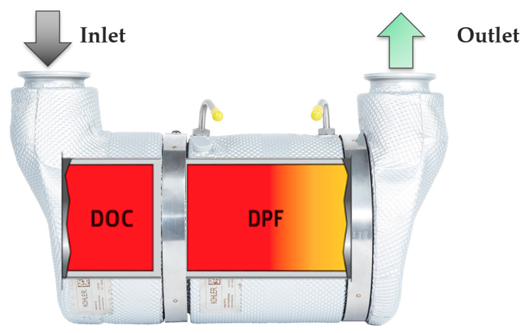
The EAS system of the KDI1903TCR is composed of a DOC and cDPF. Exhaust gas composition and temperature are tracked upstream and downstream of the two catalysts (
Figure 9). In order to calibrate the DOC and cDPF models, the following measurements have been performed at the synthetic gas bench (SGB):
DOC: Light off temperature test (Oxidation of CO, HC and NO)
DPF: Light off temperature test (Oxidation of CO, HC and NO)
The characteristic time of the EAS model is higher than the engine model so a different and, as mentioned, separate model has been created with a different time-step (1 ms for engine and 100 ms for after-treatment system) and then coupled with the engine model. The EAS is modelled as a sequence of after-treatment component sub-models (e.g., pipes, catalysts and filters). Pipes, catalysts and filters are modeled as systems with one-dimensional (1-D) discretization along the flow direction. Therefore, every system state is calculated and internally cell-wise stored. The aforementioned states include the exhaust gas and the component material temperatures, the gaseous species concentration in the exhausts, the soot loading within the filters and the storage level of absorbed or otherwise non-moving species.
The models for material and gas temperatures contain the heat conduction in the direction of the gas flow in the material and the convective heat transport by the exhaust gas mass flow. Heat exchange between material and gas is evaluated based on Nusselt correlations, whereas heat transfer to the environment considers radiation and convection. Catalyst reactions are modelled based on extended Arrhenius equations and calculated cell-wise. The extensions include inhibition terms and other cross sensitivities. Particulate filter elements (DPF) model individually the exhaust gas flow in inlet and outlet channels. These flow models are connected by a wall-flow model. Mass flow distribution along the channel is used to estimate the amount of soot deposited in the filter. This is calculated depending on soot loading in the individual cell, temperature distribution and pressure loss. In addition, the wall-flow model includes the reaction of deposited soot with oxygen O
2 and nitrogen dioxide (NO2), based on an Arrhenius approach. These reactions are paired with the catalytic reaction modelled in the catalyst models (DOC reactions in the cDPF) [
41].
2.4.1. Diesel Oxidation Catalyst Model
In this subsection, the methodology for calibrating the global kinetic DOC model is presented. An experimental campaign has been carried out on a reactor-scale sample on an SGB to fully characterize the after-treatment element. These measurements were used to calibrate the global kinetic model.
The experimental activity has been carried out using SGB tests with controlled species concentrations, mass flowrate and inlet temperature by dosing specific species in the inlet batch to minimize the interaction of each reaction on the others and thus facilitating the kinetic model calibration. An isothermal furnace was used to oven age the DOC sample, at 700 °C for 20 h, in an air mixture containing 12% of water vapor.
Table 6 reports the main characteristics of the sample:
Concentrations of species including CO, CO
2, O
2, C
3H
6, NO, NO
2 were acquired at the outlet of the sample by means of Horiba MEXA motor exhaust gas analyzers and Fourier Transform Infra-red spectroscopy (FTIR). K-type thermocouples with a sensitivity of approximately 41 µV/°C, were used to measure inlet and outlet gas temperatures. The experimental test protocol can be categorized into one main group constituted by light-off tests. They were carried out at different levels of standard space velocity (SV), on a temperature ramp from 373 K to 773 K with a constant rate of 15 K/min. The inlet feed gas composition was changed from single trace species to more complex tests, during which several trace species were included in the inlet gases volume. The standard feed composition contained 7.5% O
2, 8.5% H
2O, 0% CO
2, balanced N
2 and the trace species as reported in
Table 7.
A global reaction model has been defined for the DOC and it is shown in
Table 8. Reaction rates have been considered of first order with respect to each reactant concentration (C
xy) and expressed in an Arrhenius form, as can be seen in
Table 8 where “E
i” is the activation energy, “A
i” is the pre-exponent multiplier, “T” the catalyst temperature and “R” the universal gas constant. Finally, inhibition term (I) has been defined as in Equation (11) and included in the reaction rate expressions, to fully model the DOC behavior.
with Arrhenius terms for K
2…4. The inhibition term accounts for the negative interaction of different species on the same catalytic surface. Furthermore, the chemical reaction number 3 in
Table 8 (NO oxidation reaction) has a parameter called “keq” that is the equilibrium term depending only on the catalyst temperature and given by Equation (12):
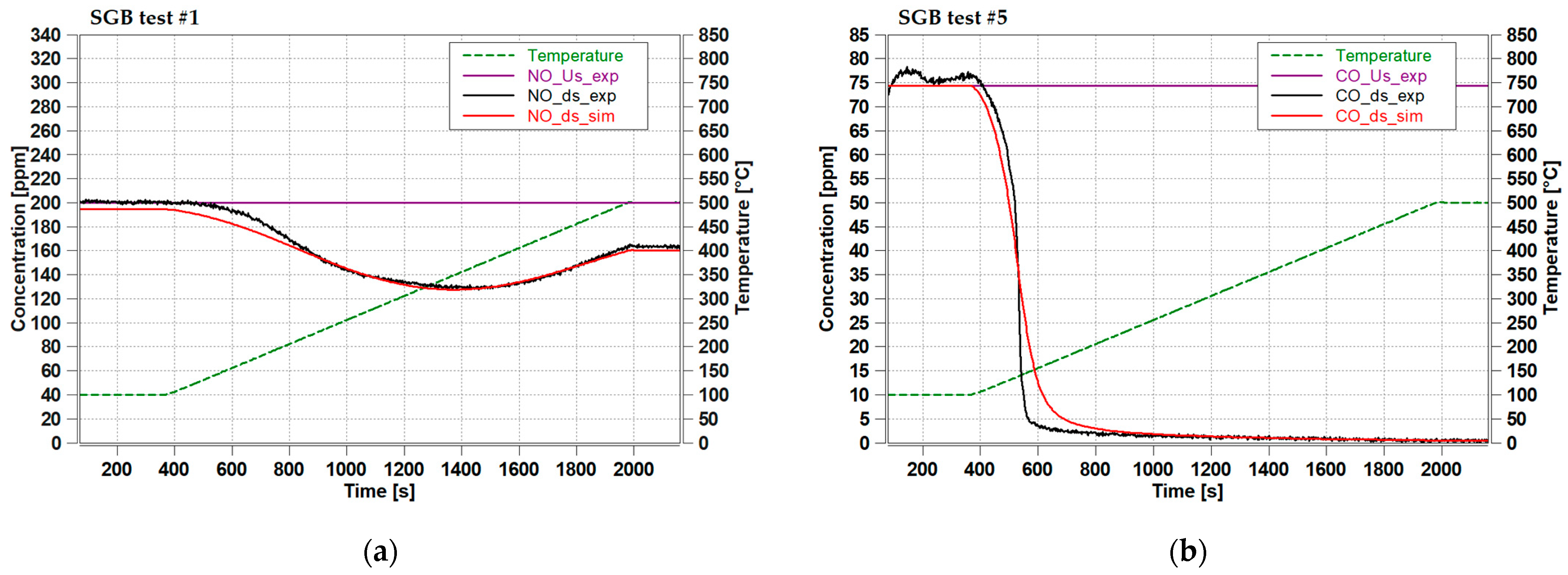
According to the test protocols, the reaction model has been categorized into different steps. In step 1, experimental data of test number 1, 2, 3 and 4 were used to calibrate NO oxidation parameters and inhibition term. This latter was defined after the calibration of oxidation reactions pre-exponent multipliers and activation energies, using data from tests with more than one trace species. In step 2, in addition to inhibition term, CO oxidation parameters were calibrated using test number 5, 6 and 8. In step 3, the calibration of C
3H
6 oxidation parameters was performed using experimental data of test number 7. To find the correct kinetic parameters, the optimizer embedded in AVL CRUISE M™ has been used to minimize the cumulative absolute error between simulated and measured outlet concentrations of different species. For each reaction defined in
Table 8, pre-exponents multipliers and activation energies were tuned and reported in
Table 9 while
Figure 10a,b show the simulation results of two different SGB tests (#1 and #5) listed in
Table 7.
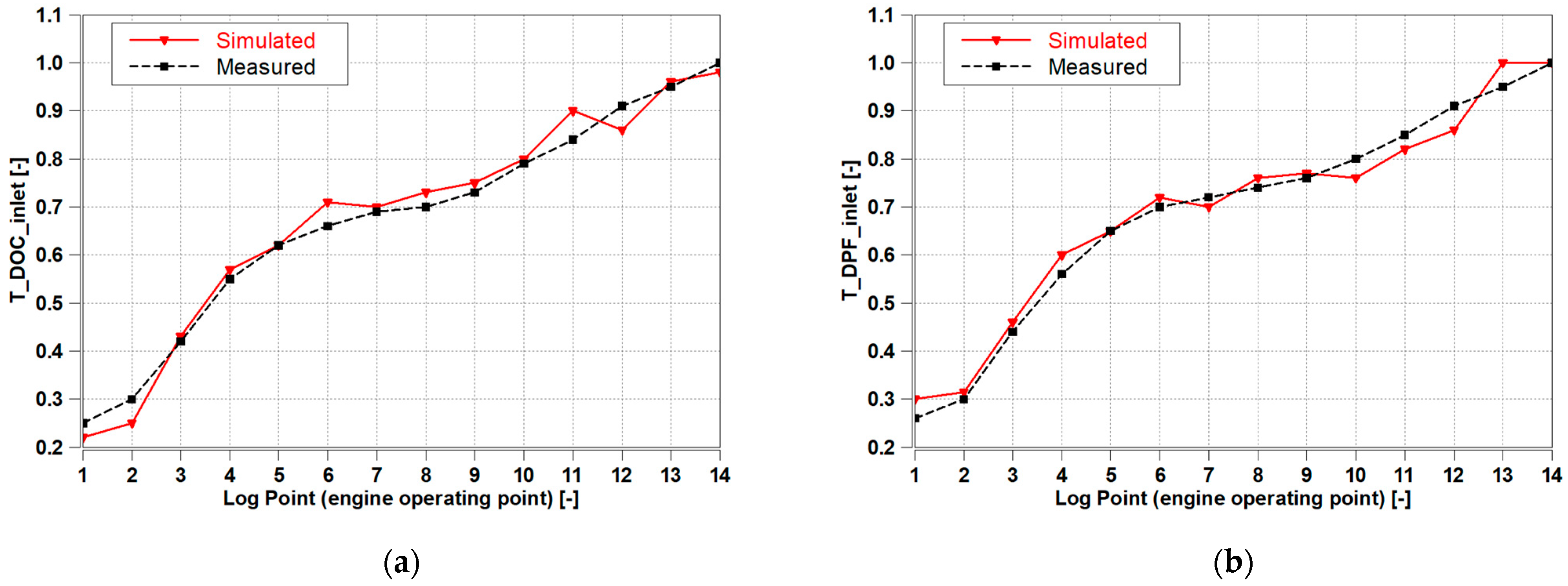
The calibrated kinetic scheme (using SGB data) was finally transferred to the full-size component model (characteristics in
Table 6) for the validation over transient cycle data, to evaluate the DOC model accuracy with real exhaust gas conditions as input. The main results are shown in
Figure 11.
The sources of different results between reactor-size and full-scale models are the following:
Non-uniformity of flow and temperature field in full-size component → affecting kinetics.
The engine exhaust gas includes a mixture of different gas species, especially hydrocarbons.
Presence of external heat transfer in the full-size component.
Different aging status of the catalyst components.
2.4.2. Diesel Particulate Filter Model
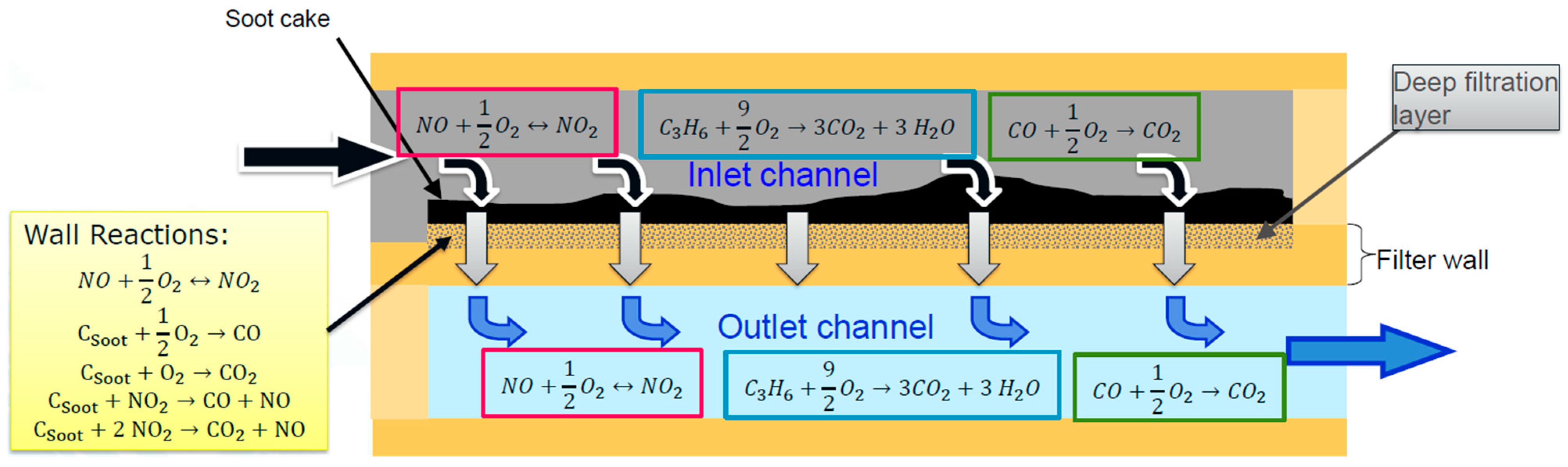
The DPF model is made of two one-dimensional flows, within inlet and outlet channels, coupled with a filtering wall (
Figure 12). Inlet and outlet channel models are similar to the DOC model: they contain the three gas reactions for NO, CO and C
3H
6 as listed in
Table 8 for DOC model.
The wall model is the DPF sub-model where soot filtration and oxidation take place. The wall is divided in two physical layers: deep filtration layer and soot cake. In each one of these layers the result of accumulation and oxidation processes are modeled: engine out produced soot is integrated to calculate the accumulation contribution and NO2 and O2 soot oxidation chemical reactions determine the oxidation process. Soot starts to accumulate in the soot cake only when deep filtration layer, which represents the porous part of the wall, is full of soot.
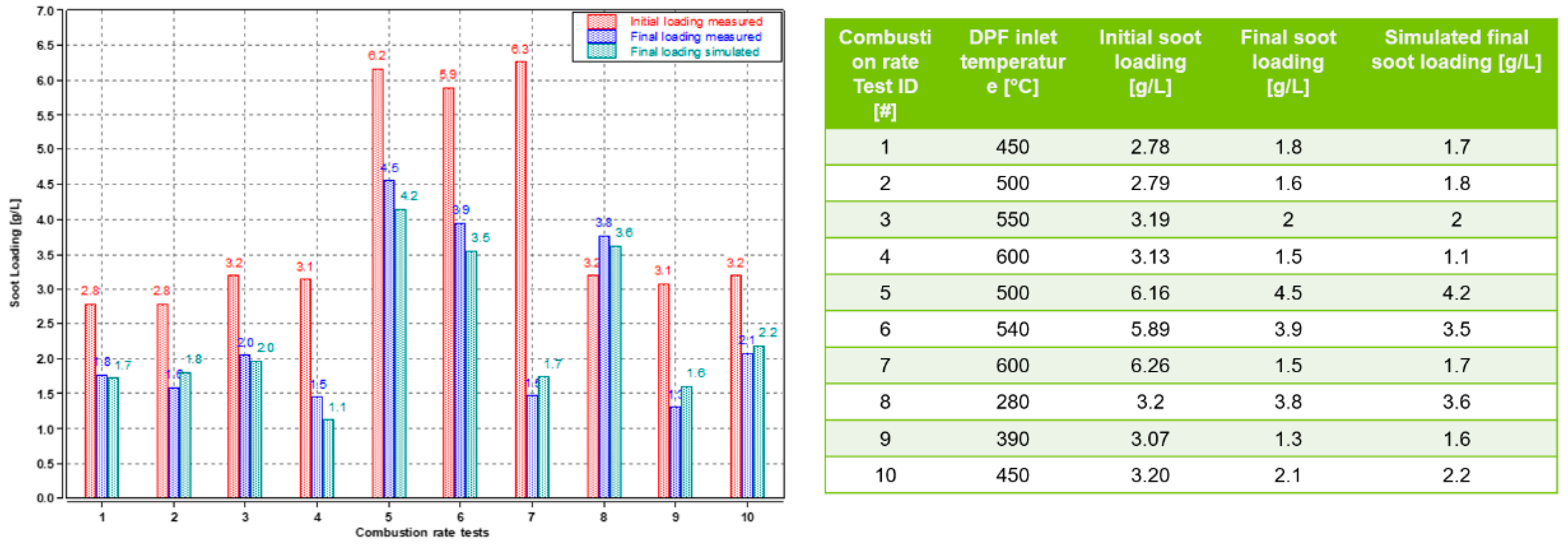
As for the DOC, an experimental campaign has been carried out on a reactor-scale sample on SGB to fully characterize the gas reactions of the filter and the procedure to calibrate the kinetic scheme was exactly the same as the DOC catalyst. After that, different tests at the real engine test bench (named combustion rate experiments) have been performed in order to parametrize the soot oxidation reactions that are the complex part of the DPF model. SGB tests on a reactor-scale sample are indeed not suitable to catch this aspect.
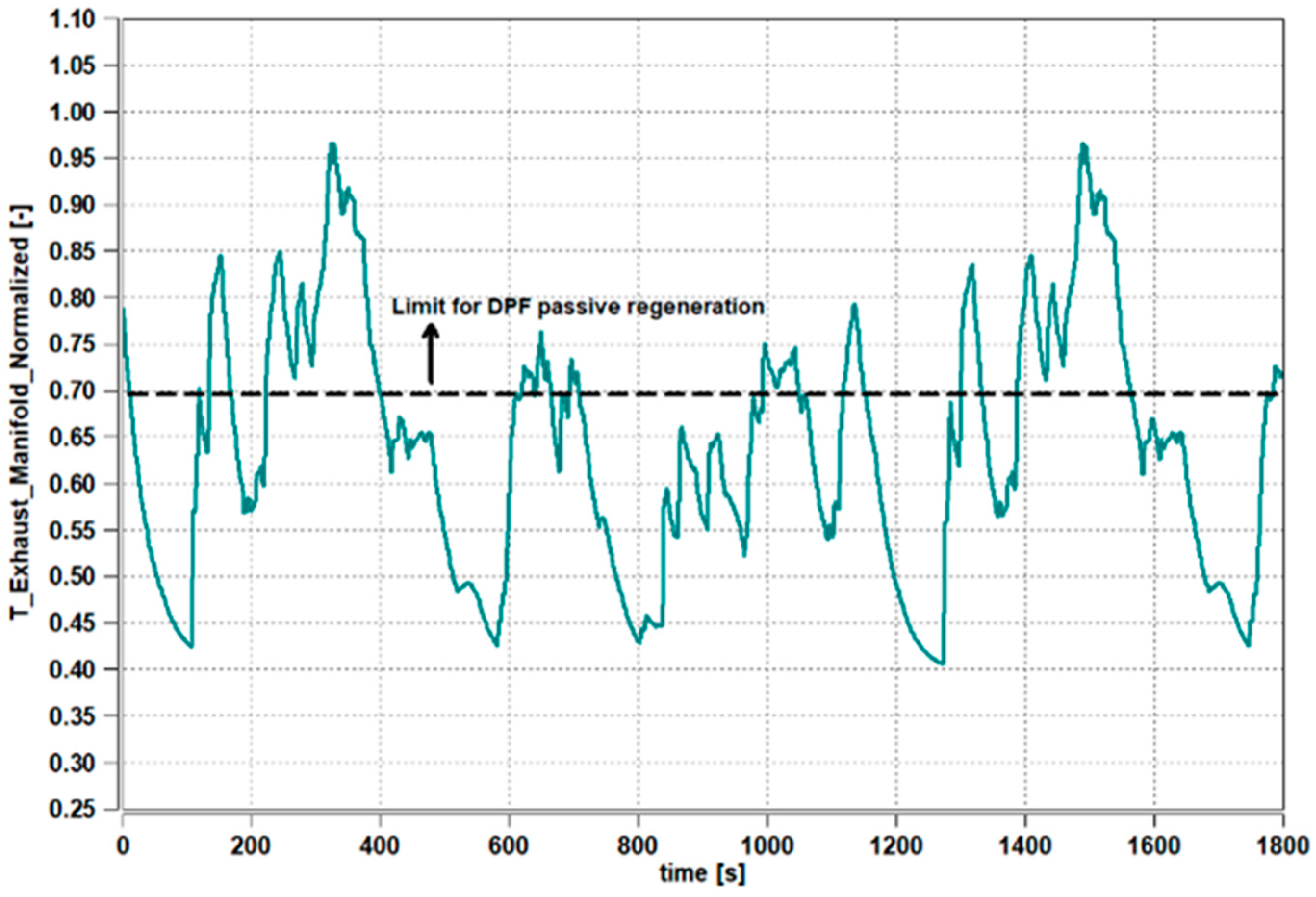
The soot mass in the DPF is reduced by regeneration reactions. These include:
Reactions of soot with O
2 (“active regeneration”) → reaction 1 and 2 in
Table 10Reactions of soot with NO
2 (“passive regeneration”) → reaction 3 and 4 in
Table 10
The reaction rates of reactions #1 and #2 detailed in
Table 10 contain the distribution factor “f
CO” between CO and CO
2 that is determined by:
with an exponent q
f1 [-] that is dependent on the oxygen concentration and “X
O2” that is the oxygen molar fraction. Similarly, in reactions 3 and 4, the distribution factor “g
CO” between CO and CO
2 is determined by:
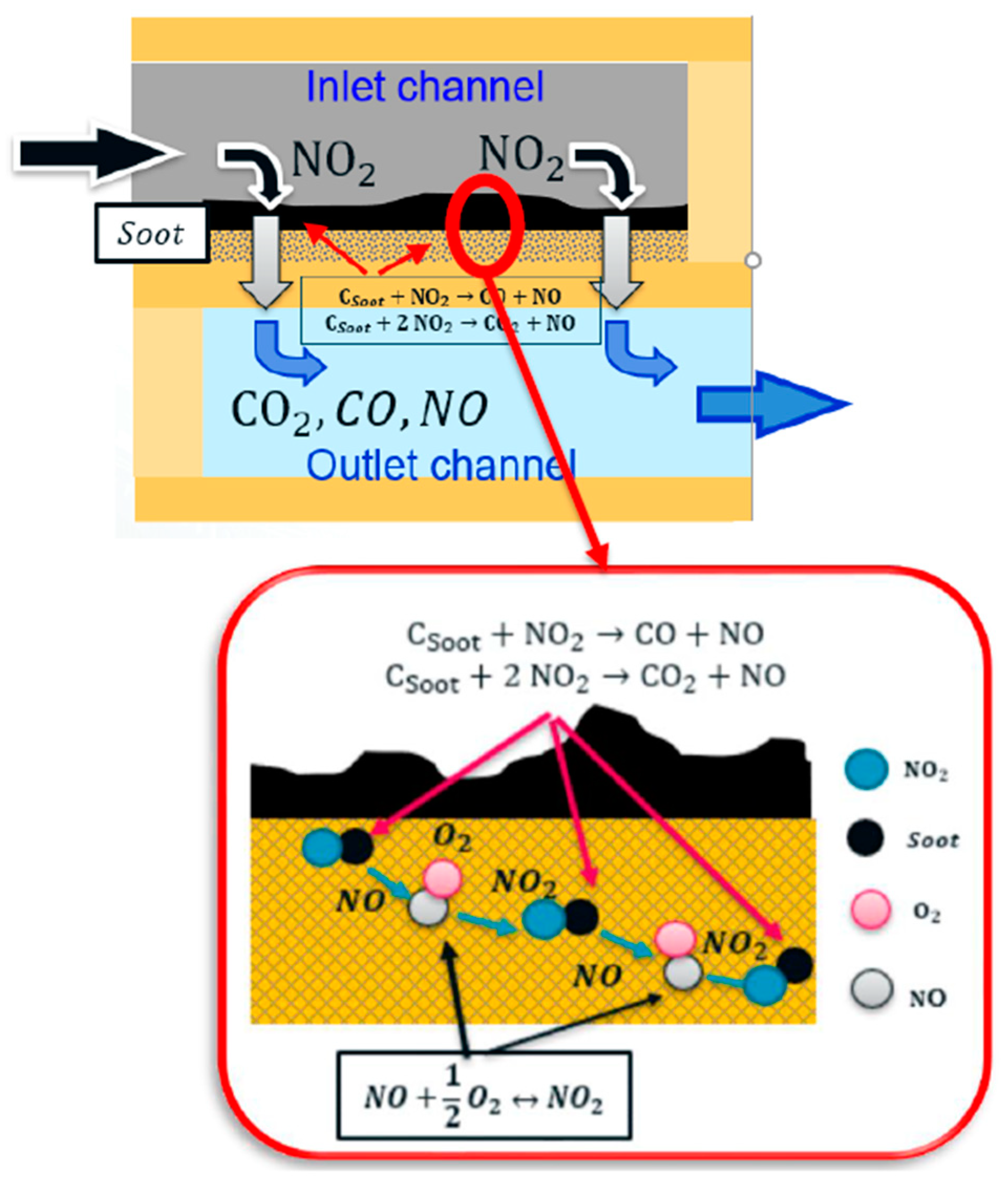
In a DPF with PGM coating concurrently to the gas-soot reactions the following NO oxidation reaction takes place:
This enables one NO
2 molecule entering the wall to oxidize more than one C-atom of the soot layer (
Figure 13). The additional NO-oxidation in the wall model leads to the fact that the NO-oxidation is modeled twice:
Both NO-oxidation reactions describe the same physical process. The need of wall NO-oxidation reaction comes from details of gas convection and diffusion at the boundary of bulk channel flow and filtration wall not having been modeled explicitly, as a semplification.
Table 11 shows the optimized values of DPF model tuning parameters mentioned above to obtain the soot oxidation simulated results, reported in
Figure 14.
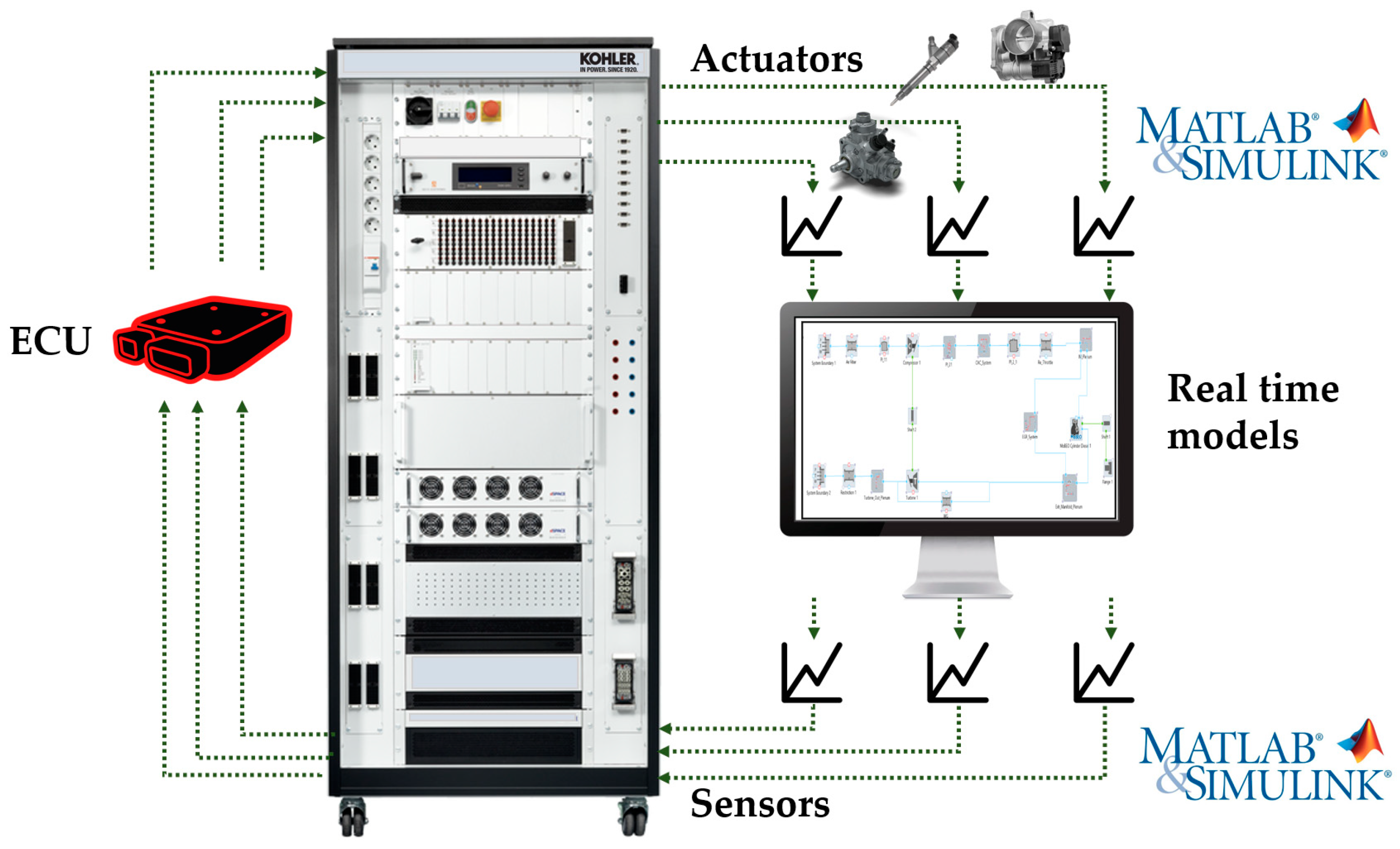
2.5. Engine Model Validation on HiL System
Once the plant models are available offline, they are compiled as Functional Mockup Unit (FMU) for the virtual test bed architecture. Subsequently, the main focus becomes the closed loop between models and real hardware (HiL real actuators in
Table 2 and engine ECU) to assure the software appropriate functioning within the virtual engine test bed as well as to check the simulation models accuracy before starting the calibration activities that are explained in the following sections.
For this research, the engine model was correlated to both steady-state data, acquired in an ICE dynamometer test bench covering the part load and full load operating points across the ICE speed range, and to non-road transient cycle (NRTC), a test cycle required for certification/type approval of Stage V engines.
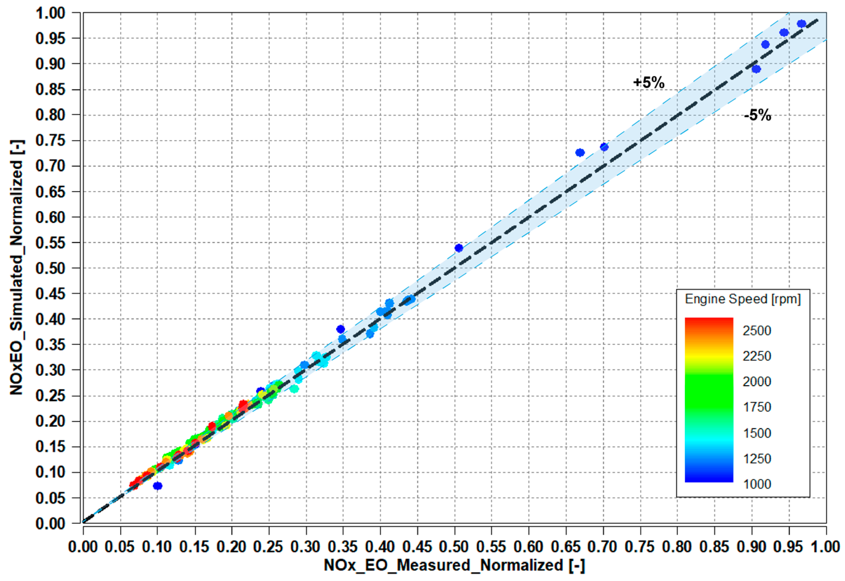
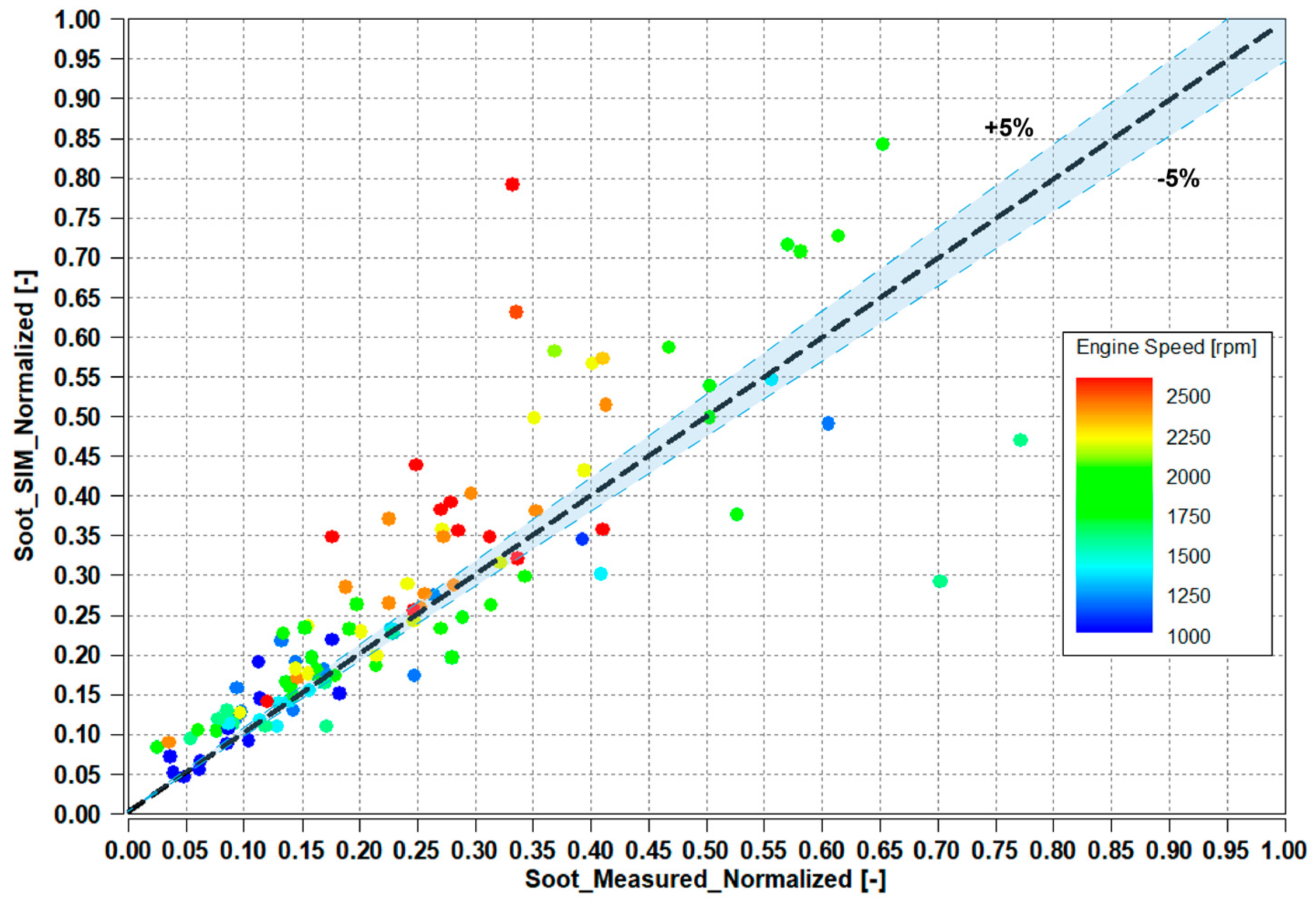
Figure 15 and
Figure 16 show a comparison of the NO
x and Soot emissions outputs from the engine in the test bed (on the
x-axis) and NO
x and Soot emissions outputs from the HiL simulation (on
y-axis). All the values were normalized with respect to the maximum value of each pollutant reached during the real test. The engine out emissions were used as main parameters for model correlation since they were input to the EAS model. For NO
x emissions, the HiL simulation model matched the test bench data within ±5% in the 98% of the tested operating points. This satisfied the correlation criteria for the NO
x emission model itself.
The higher dispersion on Soot (
Figure 16), compared to NO
x emissions, shows the difficulties in defining an accurate soot model since it depends, more than other emissions, on multiple factors subject to significant engine-to-engine variance. Moreover, local deviations can be explained by highly transient effects that are difficult to replicate on the HiL system.
However, even if the correlation between simulation and test is less satisfactory for soot than it is for other variables, the number of simulated points is in a “safety region” because the simulated soot overall overestimates the real one. Therefore, results have been considered viable.
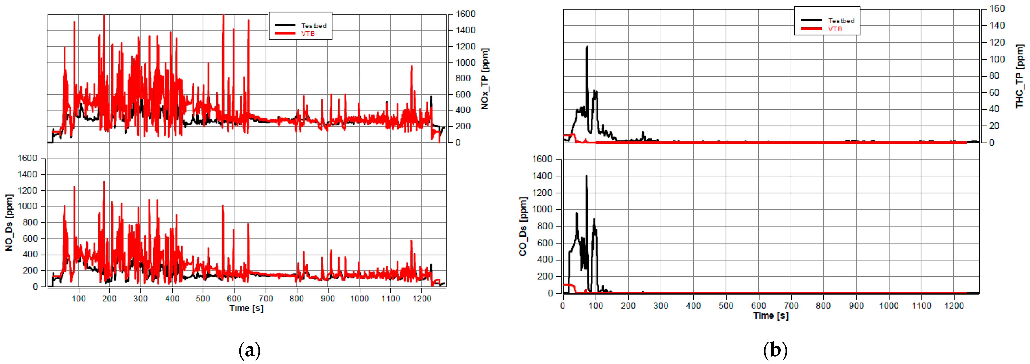
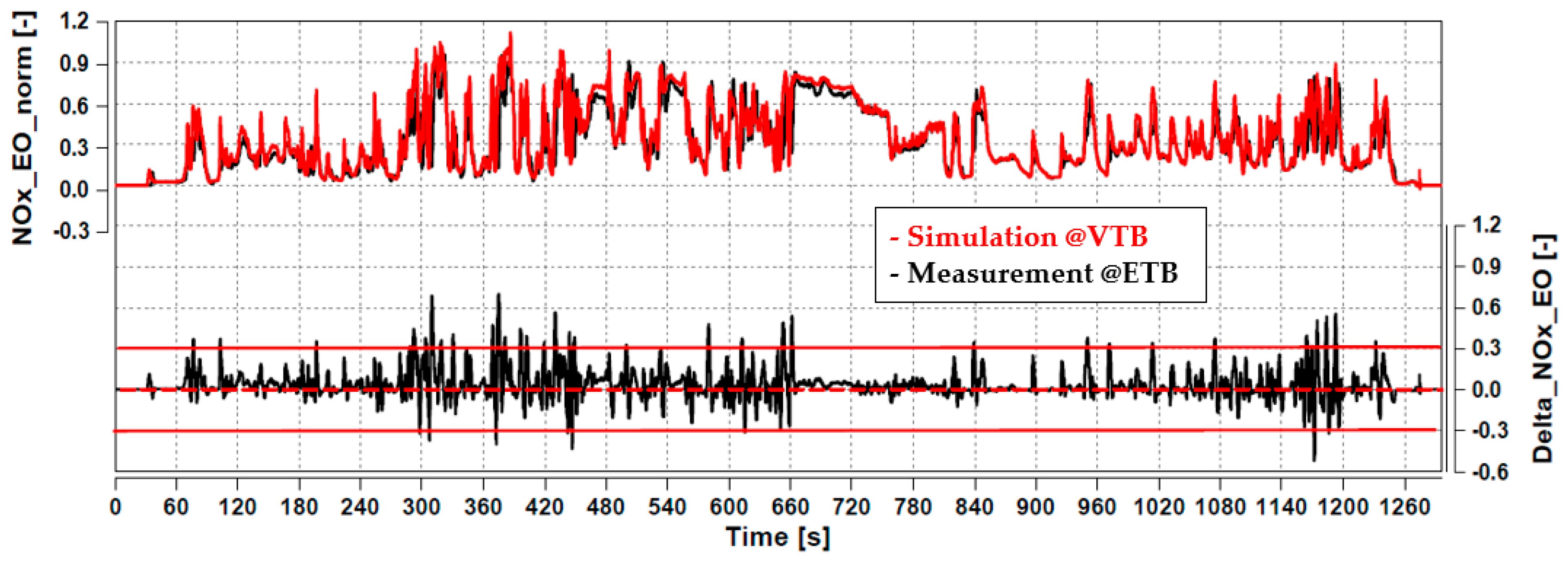
Figure 17 shows a comparison between NO
x emissions measured at Engine Out (EO) over the transient cycle (NRTC) and NO
x emissions at EO simulated at VTB. The signals are normalized with respect to the maximum NO
x experimental value reached during the cycle. In the second row of
Figure 17, a difference between simulated NO
x trace and measured NO
x signal has been reported to better visualize the instantaneous errors.
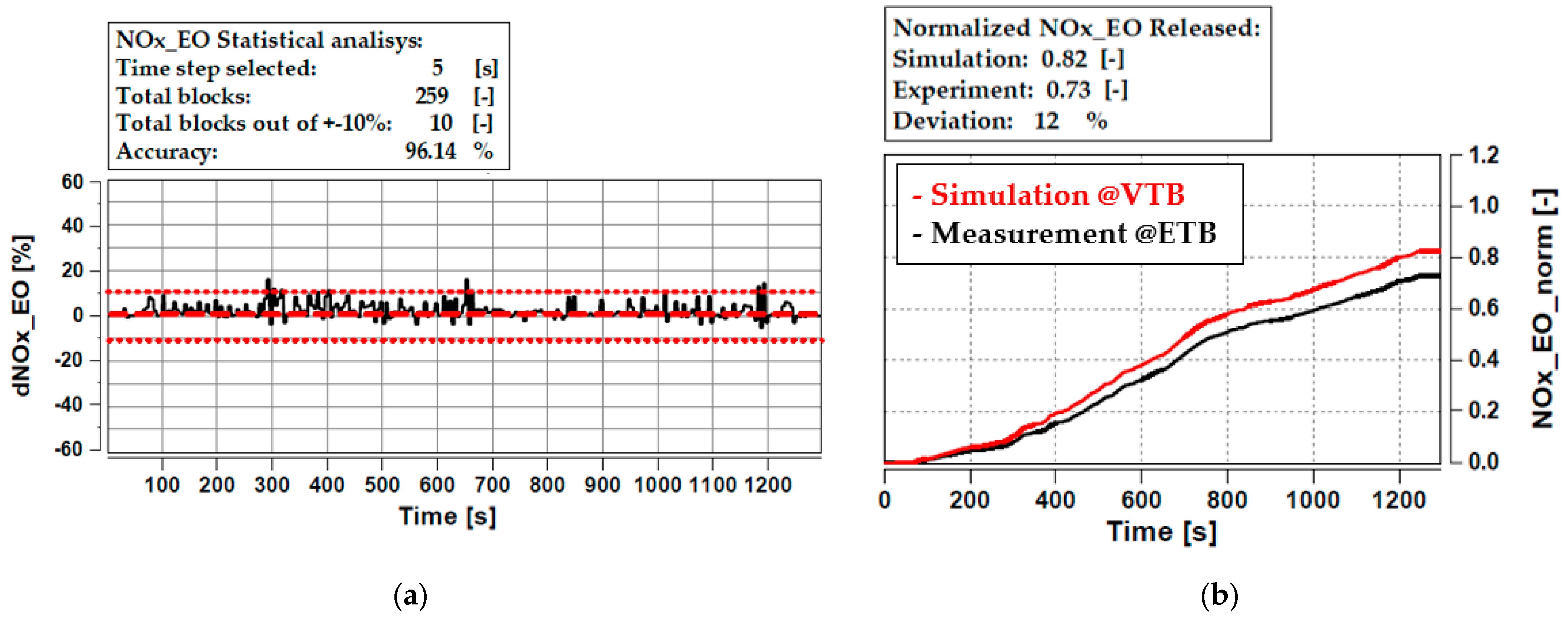
To estimate the accuracy of the engine model running over the NRTC, a statistical analysis has been carried out. In
Figure 18a the transient cycle is divided into five seconds blocks. Each block is treated as an independent block and the integration of time-based values is performed. The weighted deviation “dNOx_EO” is calculated taking into account the final accumulated value at the end of the cycle (measurement) and the relative integrator time with respect to the end (Equation (16)):
An indicator of the simulation predictive reliability over the whole cycle can be arrived at counting the quota of blocks within the boundaries of a ±10% error interval (96.14%). Moreover, the accumulated NO
x emission simulated over the NRTC (
Figure 18b) shows a good agreement with respect accumulated NO
x measured at ETB.
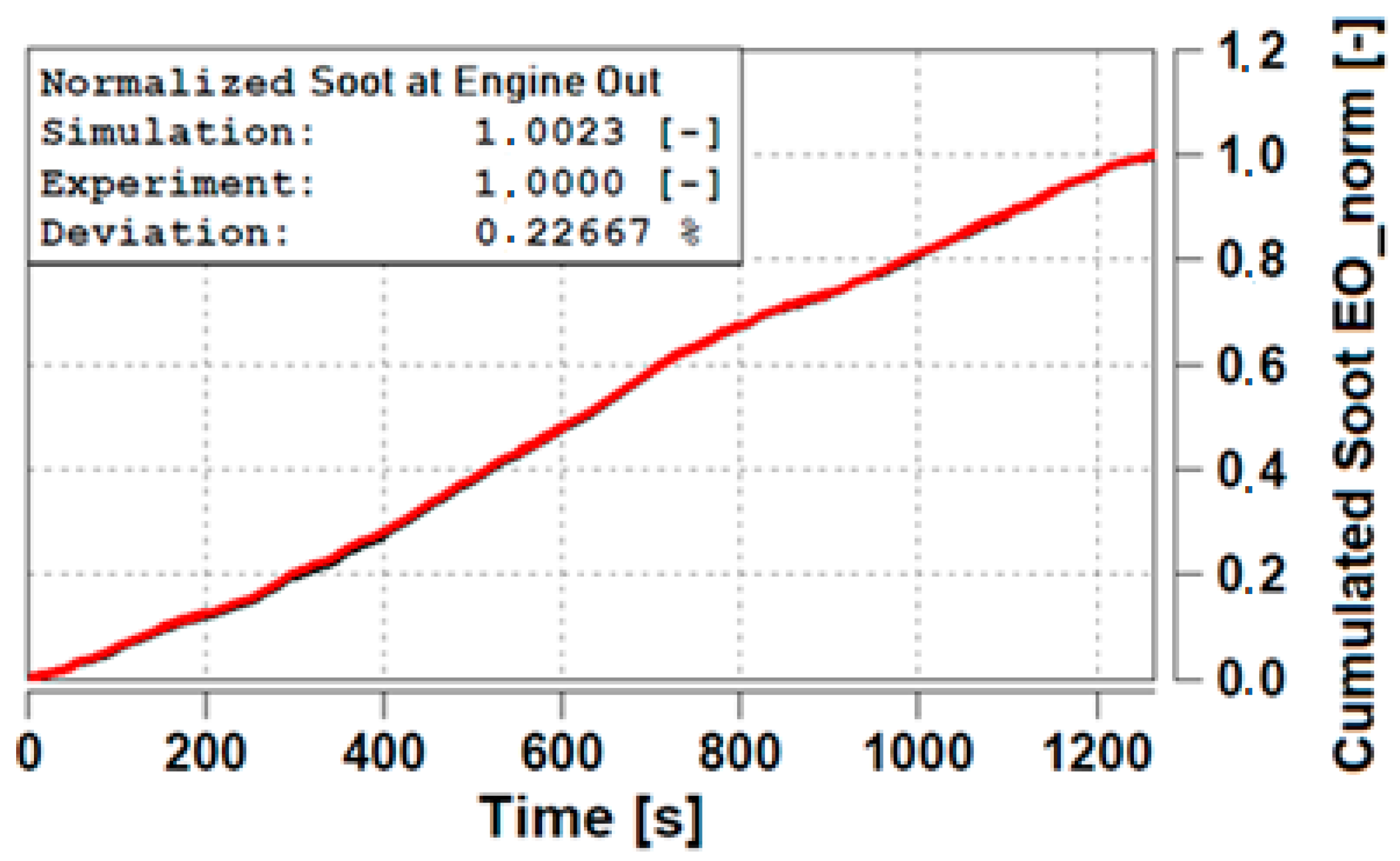
The same statistical analysis has been performed for soot emission. However, for the sake of brevity only the accuracy on the accumulated soot is being reported here.
Figure 19 shows the accumulated soot at engine out over an NRTC cycle (normalized with respect to the maximum experimental value reached during the transient cycle), showing a very good agreement between test and simulation, and thereby proving the viability of the HiL system to simulate the soot loading.
Soot loading is certainly one of the most critical variables to be looked in off-road applications because it is directly linked to the cDPF regeneration strategy and so it directly impacts machine productivity. In fact, soot needs to be burned off to regenerate the cDPF, very often while the machine is at a standstill (active regeneration). Thanks to simulation accuracy achievable through the methodology hereby detailed, it is possible to optimize the ECU calibration strategy directly at VTB, so as to minimize the need for active regenerations, limiting downtime and keeping end-user machinery operational and profitable.
Similar validation work was carried out for the EAS model as well.


