Abstract
Faults and unintended conditions in grid-connected photovoltaic systems often cause a change of the residual current. This article describes a novel machine learning based approach to detecting anomalies in the residual current of a photovoltaic system. It can be used to detect faults or critical states at an early stage and extends conventional threshold-based detection methods. For this study, a power-hardware-in-the-loop approach was carried out, in which typical faults have been injected under ideal and realistic operating conditions. The investigation shows that faults in a photovoltaic converter system cause a unique behaviour of the residual current and fault patterns can be detected and identified by using pattern recognition and variational autoencoder machine learning algorithms. In this context, it was found that the residual current is not only affected by malfunctions of the system, but also by volatile external influences. One of the main challenges here is to separate the regular residual currents caused by the interferences from those caused by faults. Compared to conventional methods, which respond to absolute changes in residual current, the two machine learning models detect faults that do not affect the absolute value of the residual current.
1. Introduction
1.1. Background
In earth-grounded power supply systems, the use of residual current devices (RCD) has been an effective means of protecting people, animals and installations from damage caused by currents flowing through bodies and ground earth if they exceed critical values. In addition, residual current monitors (RCM) offer the possibility of monitoring currents flowing through earth with the same procedure and sending a message if adjustable threshold values are exceeded. Both types of devices record the sum of the currents flowing to and from active conductors. If the sum of currents is not equal to zero, there are usually undesired currents flowing back to the source via the body and earth, which are generally referred to as differential currents (also known as residual currents) [1].
In earlier times, residual currents were essentially caused by insulation faults in systems and were thus referred to as fault currents. Today, due to the enormous increase in non-linear electrical loads, as well as regulated power generation systems such as photovoltaic (PV) systems with their high-frequency controlled current converter stages, we also see massive amounts of so-called operation-related leakage currents taking the same path as fault currents. Measures to ensure electromagnetic compatibility (EMC) often divert interference currents against the earth potential and amplify the operational leakage currents, which can have frequencies of up to 150 kHz. Furthermore, modern electrical loads such as generators contain direct-current (DC) circuits with high voltages that can also generate DC fault currents.
1.2. Motivation
Modern residual current circuit breakers and residual current monitors (see Table 1) map the residual current (that is, operational leakage current + fault current) with the help of their active summation current transformer as a total RMS value of the geometric addition of the different frequency components. In simplified terms, the calculation is as follows:
where represents the effective differential current, the leakage current and the fault current. Due to the physically determined geometric addition of the residual current components, this results in different constellations, for example, the challenge of being able to detect a low but critical fault current in a system with a high leakage current component.

Table 1.
Overview of state-of-the-art systems to detect and analyse residual currents.
A new generation of smart RCM are using the residual current data frequency, selective over a broad frequency range. This makes it possible to achieve completely new protection concepts that minimize failure, fire, corrosion and other risks. Thus, in addition to the sum effective signal, effective values of discrete frequencies and frequency ranges are extracted from the residual current signal. This approach makes it possible to separately detect a very small fault current, for example, at 50 Hz or DC, despite a high leakage current in high-frequency ranges.
1.3. Contribution
This article describes a machine learning based approach to analyse the residual current on the AC side of a grid-connected PV system over a broad frequency range in realtime. The approach combines a smart RCM sensor system with two machine learning algorithms (pattern recognition and variational autoencoder). The goal of this approach is either to automatically adapt to different environmental conditions as well as to prematurely detect faults or critical states (“predictive maintenance”) in grid-connected PV systems to enhance the functionality of modern detection methods. Section 2.1 briefly describes the input data used for the analysis followed by Section 2.3 and Section 2.4 describing the principle of the used machine learning algorithms. The laboratory experiments are described in Section 2.5 and Section 2.6 of this article followed by the test results representing pure fault patterns in Section 3.1 and the results of the algorithm training and fault detection in Section 3.2. The terms failure, fault and error are used in the sense of the terms defined in [2].
1.4. Related Works
Stylianos et al. [3] briefly discuss identification methods detecting faults on the DC side of a PV system. Various fundamental strategies, such as I–V curve analysis and machine learning approaches, are compared regarding efficiency, reliability and economic aspects. Another brief overview about typical faults as well as machine learning based detection algorithms in PV systems is given in Kumaradurai et al. [4].
Fazai et al. [5] use a Gaussian process regression (GPR)-based generalized likelihood ratio test (GLRT) named approach to detect faults such as bypass diode and mismatch faults on the DC side of a grid-connected PV system. The approach measures and analyses the output values (DC voltage and current) of a PV array. Principle component analysis (PCA) in combination with support vector machines (SVM) to detect especially incipient faults on the DC side is shown in Attouri et al. [6]. In this work, experiments were conducted variating the line to ground resistance in a PV system. The methodology of PCA for fault detection and diagnosis is also used in Hajji et al. [7], where several faults on the DC and on the AC side of an emulated grid-connected PV system have been injected. Supervised machine learning approaches have been used for analysing the system’s common signals (DC and AC output voltage and current).
2. Methodology
2.1. Dataset
The analysed dataset consists of residual current data, which are measured using a closed loop ferrite sensor with multiple magnetic coupling circuits for different frequency bands (see Table 2). The data are sampled at a rate of . All measures are taken in a range from 1 mA–30 A separated into three, automatically switched measurement ranges (0–3000 mA, 3000 mA–10,000 mA and 10,000 mA–30,000 mA). The applied accuracy per range is at least or better. The collected data are transmitted to a cloud-based machine learning environment at an interval of 1/s.
Table 2.
Measured sensor channels.
2.2. Input Data Preparation
For data processing, the sensor values are collected and converted into SI units representing floating point numbers. After acquisition, the samples are stored in a database together with the timestamp of the measurement. The sampling period is not constant, but is in the range of 1 s. There is also model-specific data processing, which is described in the subsections for the two machine learning methods used in this project. The following is true for both models:
- Resampling: Due to the varying sampling period it is necessary to convert the data to a dataset with a constant sampling period;
- Removal of duplicates;
- Filling of missing values. Forward filling, followed by backward filling is used.
2.3. Pattern Recognition
The “Anomaly Factor Estimator” algorithm attempts to generate a set of valid hypotheses for each time of day and type of day. A hypothesis is defined by the pattern of data from the time series and by what period of the day it may occur and how many times it was seen.
The analysis of the training data first starts with the segmentation of the time of day. Each segment found contains a pattern that can occur in its time range. If a similar pattern is not already present in the hypothesis set, the hypothesis set is expanded. This process is repeated for each day of the same type and for each day type (e.g., days with different solar output). In the end, a set of hypotheses is obtained in which each time-of-day hypothesis is defined by a set of segments. Since there is no guarantee that the training data itself is free of anomalies, the next step is to clean the hypothesis space. In this case, hypotheses of the same time segment are compared. Highly discrepant hypotheses are removed from the hypothesis space. The third step of training is to find a threshold above which a model defines a deviation as an anomaly. This process is performed by a simple pass through each hypothesis space. Each hypotheses from its hypothesis space is compared to the other hypotheses in the same space to evaluate the deviation, and the respective maximum of the deviation of the anomaly factor is defined as the threshold.
When analysing the measured realtime data, the model finds possible hypotheses for each data point at that time. For each hypothesis, the model compares the hypothesis pattern with the actual pattern and calculates the anomaly factor. The comparison of the patterns is done by comparing the maximum, minimum and mean of the two patterns. The result is the minimum value of the anomaly factor of each hypotheses for that time of day. This value of the anomaly factor is very unstable, so smoothing is performed with a low-pass filter. If the new value is higher than the previous one, the change of the anomaly factor is faster, if it is lower, the change is correspondingly slower.
In the next step, the model tries to evaluate the reliability of the analysis and the state of the model. To evaluate the reliability, new unknown data sets are compared with the training hypotheses during runtime and new hypotheses are formed if necessary. For a specific estimate of the reliability of the anomaly factor, both hypothesis spaces from new data and training data are compared by calculating the variance. The more similar the two hypothesis spaces, the more reliable the output of the anomaly factor. While the reliability of the analysis or the anomaly factor is only evaluated on the basis of the subsets of the hypothesis spaces, the evaluation of the model or health status is based on the entire hypothesis space. Here, the variance between training hypotheses and runtime hypotheses also provides information on the extent to which the current overall model deviates from the original model. Shortly after training, the variance is 1, since training hypotheses and runtime hypotheses are almost the same. The more the system to be monitored deviates from the original system due to external influences, the lower the variance. If this value falls below a defined threshold, the model is trained again using the new data (model retraining).
2.4. State Estimation
The state estimation model has two combined purposes: (1) to learn and predict a distinct state representation of the system under observation; and (2) to detect anomalies in the observations.
Learning a state representation [8,9] for an electrical system like a production plant or a solar inverter requires learning a mapping function from the measured multivariate electrical input data (residual current measurements) to estimate modes of operation of the system. Such a mapping function has to meet certain objectives. In our use-case one key objective is to find latent states for disjoint operational modes of the system. An alternative objective could be to identify generative factors, which correspond to on-off states of individual machines or system parts. The later objective is aligned to methods in the area of unsupervised non-intrusive load monitoring (NILM), while the first objective is considered more suitable for the conducted experiments. A classical approach to find a mapping function is to apply a dimensionality reduction method on the multivariate input data and to perform a clustering on the reduced state representation. However, classical dimensionality reduction methods like principle component analysis (PCA) [10] follow unsuitable objectives (e.g., maintain variance) instead of preserving information for disjoint modes of operation.
2.4.1. Variational Autoencoder
To gain control over the objectives of the state mapping function, the method of autoencoders [11] has been selected. Autoencoders are machine learning models which learn to represent multivariate input data through an intermediate latent space representation. The latent space representation can have a smaller dimensionality than the input data dimensionality. With a smaller latent space, an autoencoder performs the combined task of dimensionality reduction and state mapping. Autoencoders provide already some level of control over the objectives for latent space representation via regularization (e.g., sparsity of latent space values). However, regularization provides only limited influence on the properties of the selected representation in the latent space. Recent work on variational autoencoders [12] has focused on finding state representations, which are based on an estimation of disjunct generative factors for the observed input data. A variational autoencoder enforces a very dense representation of the input data in the latent space. Under such constraints, individual elements of the latent space tend to represent the activity of each of the generative factors. A variant of variational autoencoders, the beta-VAE [13], provides even better control of the goal of the mapping function by providing a parameter beta that controls whether the model focuses either on reconstructing the input data or on separating the generative factors. It has been shown in [14] that a dense representation of a variational autoencoder favours a separated placement of generative factors in dimensions of the latent for certain use cases. This is also the main driver to select a beta-VAE for learning a state representation for the electrical input data.
In the next step of the processing pipeline, the generated state representation values are clustered to identify states which are found frequently in the training data. The resulting clusters are used as training data to classify new state representation values. Since the placement of states in the state representation space is stochastic when using a VAE, a post-processing step of state labels is done by reordering the states in a way that states with a high interconnection are close together in the label space (states are labelled with integers).
2.4.2. Anomaly Detection
Besides estimation of a state mapping, autoencoders also provide the basis for anomaly detection (2). Autoencoders are trained to reconstruct the input data on the output neurons. For new unseen input data, a reconstruction is calculated and the difference between the input data and the predicted reconstruction is evaluated (reconstruction error). This error produces a useful signal for the detection of anomalies. The higher this scalar error value is, the more likely it is that the distribution of the input data is not part of the training data.
The resulting data processing pipelines for training and prediction are shown in Figure 1. During training (Figure 1a), the multivariate sensor input data are transformed, cleaned and resampled to a 1min period to prepare the data for the autoencoder training. The autoencoder model is then fitted by applying the data to the inputs and the outputs of the symmetrical autoencoder neural network. Using a gradient descent based optimizer, the autoencoder learns to reconstruct the input on its output neurons. The centre of the autoencoder contains a narrow layer of neurons called the latent space. The narrowness of this layer forces the autoencoder to learn a compressed representation of the input data, since it has to reconstruct each input sample through this narrow vector space. After the training of the autoencoder, the compressed representations of all input samples from the training data are taken and a k Means clustering is performed over those state representation values. Those clusters represent the estimated states of the system observed. Finally, the states are ordered to give states a numerical representation which represents close proximity of occurrence. The clustering result and the state transformation table are stored in the model. For prediction (Figure 1b), new data samples are transformed and resampled and are then fed into the autoencoder. The resulting reconstruction is used to calculate a relative reconstruction error. The compressed state representation is taken from the latent space, transformed via the stored table and delivered as a state estimation. In the context of this project, the training and evaluation of the model has been performed in two different configurations. In the first configuration, the complete time series is used for training, including the phase of normal operation and the phases with injected faults. The resulting model is used to evaluate the phases with induced faults. In the second configuration only the data from normal operation is used for training and the evaluation is conducted for the phases with injected faults.
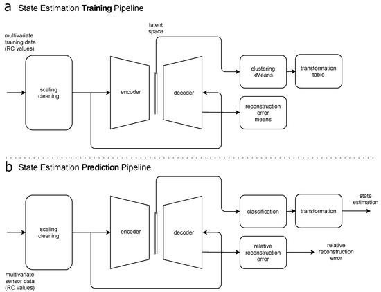
Figure 1.
Simplified models of the data processing pipelines: (a): Principle of the state estimation training pipeline. (b): Principle of the state estimation prediction pipeline.
However, it is obvious that in the first configuration it can be assumed that there is a higher probability to identify the different faults as different states, while in the second configuration the effects of injected faults would be more likely identified as anomalies with increased reconstruction error.
2.5. Experimental Data Acquisition
The experiments discussed in this article have been mainly performed with a Power-Hardware-in-the-Loop (PHIL) setup using a Regatron TC.ACS grid simulator and two Elektro-Automatik EA91000PSI DC sources. As Device-Under-Test (DUT) a SMA Sunny Tripower 15000kTL-30 PV inverter has been chosen. Figure 2 shows the principle of the test setup.
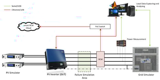
Figure 2.
Principle of a Power-Hardware-in-the-Loop test setup used to physically emulate faults in a grid-connected PV system and to analyse the effect of those faults on the residual current.
The grid simulator provides stable, non-fluctuating grid conditions needed to eliminate the uncontrolled effects on the residual current from the public grid. In this case, the simulator is a semiconductor based power amplifier with a nominal output power of [15]. For the tests, standard grid conditions with an RMS voltage of (phase-neutral) and a frequency of have been chosen. To add a more realistic grid behaviour to the setup, the neutral has been grounded during the whole experimental period.
The DC sources [16] are used, running in PV simulator mode to provide the input power for the DUT. For the experiments, a standard PV curve as shown in Table 3 has been set.
Table 3.
Photovoltaic simulator parameters used to simulate the irradiation behaviour of a typical PV plant.
The residual current has been measured with an RCM sensor DCTR B-X Hz 035-PoE [17] installed on the DUT side of the fault emulation area.
2.6. Scenario Description
Table 4 shows five fault scenarios that were physically emulated in the laboratory experiments. In the following Section 2.6.1, Section 2.6.2, Section 2.6.3, Section 2.6.4 and Section 2.6.5, the causes of the errors and the detailed implementation of those are discussed.
Table 4.
Overview of the physically emulated fault scenarios in the laboratory experiments.
2.6.1. Scenario 1: Instantaneous Increase of the Capacitive Resistance
The cause of an increase in capacitive resistance is, among other things, the degradation of the insulation due to ageing and external influences such as moisture or contamination. In this case, the cable to ground capacitance increases with time. To emulate this effect, external capacitors, connected between line and ground, with values from C = 0.22 nF to C = 680 nF are used (Figure 3).
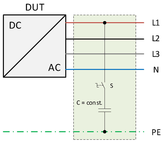
Figure 3.
Physical emulation of faults in an inverter based energy system: Instantaneous increase of the capacitive resistance between line and ground.
2.6.2. Scenario 2a: Instantaneous Decrease of the Ohmic Resistance
Ground faults and short circuits due to cable damage cause an immediate change in the ohmic resistance between the affected lines. To emulate this behaviour, variable power resistors have been connected between line and ground as shown in Figure 4.
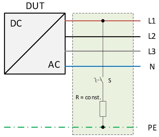
Figure 4.
Physical emulation of failures in an inverter based energy system: Instantaneous decrease of the ohmic resistance between line and ground.
2.6.3. Scenario 2b: Gradually Decrease of the Ohmic Resistance
Responsible for a relatively slow decrease of the ohmic resistance from line to ground over the time is, among other things, the degradation of the insulation due to ageing and outside influences like humidity or soiling. Manually decreased variable resistors are used to investigate the effects of those creeping failures on the residual current (Figure 5).
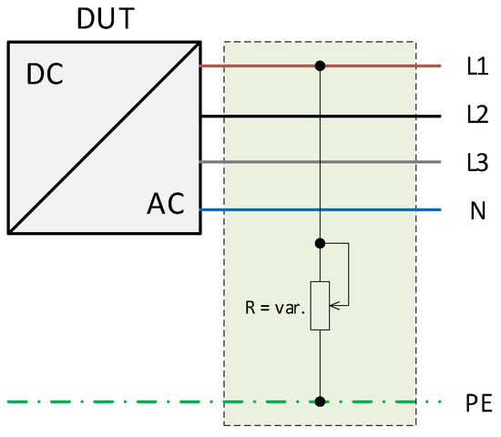
Figure 5.
Physical emulation of faults in an inverter based energy system: Slow decrease of the ohmic resistance between line and ground.
2.6.4. Scenario 3: Increased Series Resistances and Broken Lines
Line breaks are often a result of long-term mechanical stress and can lead to arcing and fires (Figure 6a). On the other hand, preceding deterioration of connections due to corrosion can lead to an increase in series resistance (Figure 6b). This leads to a sharp rise in temperature at the point of increased resistance and ultimately to a greatly increased risk of fire.
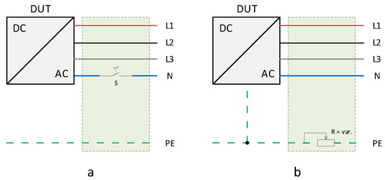
Figure 6.
Physical emulation of faults in an inverter based energy system: (a): Instantaneous disconnection of the neutral line N. (b): Slow increase of the ohmic series resistance of the ground potential PE.
2.6.5. Scenario 5: DC Electric Arcs
Arcing due to cable damage or contact problems can cause dangerous secondary effects such as fires, especially in DC circuits. To determine the effects of arcing in a DC circuit on the fault current, experiments were conducted using a special experimental setup (Figure 7) to generate arcs. A simple DC source with a constant output voltage is used in combination with an arc generator consisting of two separable copper wires. The arc is generated in parallel with a resistor .
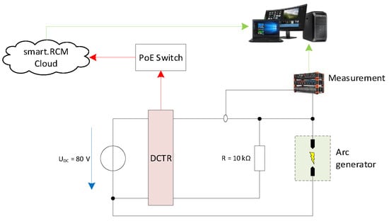
Figure 7.
Principle of a test setup used to generate arcs in a DC system to analyse the effect of those on the residual current.
3. Results and Discussion
The experiments are divided into two main phases. In the first phase, the pure effects of the injected faults on the residual current shall be determined and analysed. Therefore, parasitic influences have been minimized by operating the DUT in constant voltage mode with a fixed DC voltage without any redundant control algorithms. The results of this experiments are discussed in Section 3.1. Subsequently, in the fault detection phase, the DUT has been provided with an input power time series representing a typical irradiation curve to achieve a more realistic behaviour. In this phase, some of the faults have been reproduced to determine if the algorithm is able to detect these faults. The results are discussed in Section 3.2.
3.1. Fault Patterns
3.1.1. Scenario 1: Instantaneous Increase of the Capacitive Resistance
As shown in Figure 8, the residual current increases at relatively high capacities esp. in the frequency ranges and . Capacities do not have a visual effect. The DC part is also not affected.
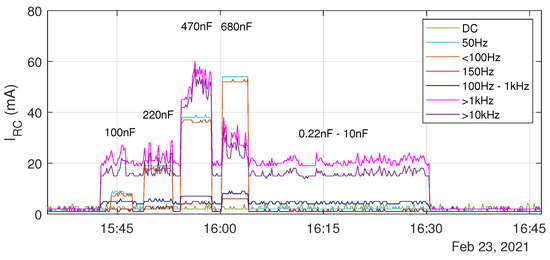
Figure 8.
Experimental results of scenario 1: Behaviour of the residual current depending on immediately switched capacitors between line and ground.
3.1.2. Scenario 2a: Instantaneous Decrease of the Ohmic Resistance
As a result of this experiment, Figure 9 shows the behaviour of the residual current when external resistors are immediately switched between line and ground. Down to a resistance the current increases rapidly in the frequency range , while the upper frequency ranges and the DC part are not affected. At resistances , the residual current increases over the whole observed frequency range including DC.
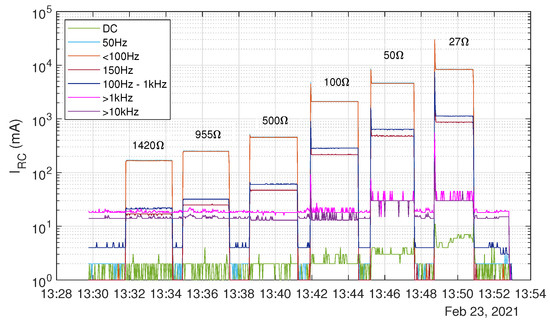
Figure 9.
Experimental results of scenario 2a: Behaviour of the residual current depending on immediately switched resistors between line and ground.
3.1.3. Scenario 2b: Gradually Decrease of the Ohmic Resistance
Analogue to the experiment before, the residual current in the lower frequency ranges gradually increases with the decrease of the resistance. At resistances lower than , also the higher frequency parts and the DC part are affected, as shown in Figure 10. In this case, the resistances started at (1) respectively (2) and have been manually decreased to an end value of (1) respectively (2). Notably, the higher frequency ranges do not show the same gradual increase than the lower frequency ranges and DC but are limited to a certain value. The cause for this behaviour can be explained with the switchover to another measuring range of the used DCTR sensors. The spikes on the graph at ≈ [30 mA, 100 mA, 300 mA, 1 A, 3 A] can be also tied to the adjustment of the measuring range.
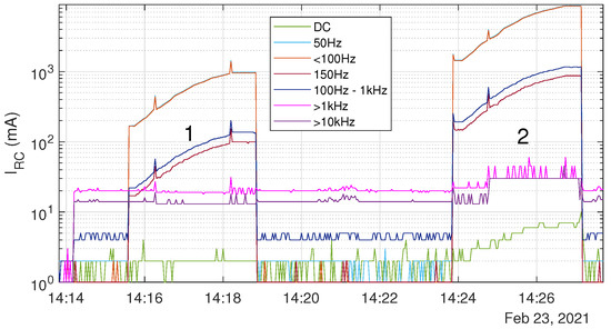
Figure 10.
Experimental results of scenario 2b: Behaviour of the residual current depending on slowly decreasing resistances between line and ground. 1: Resistance decreased from to . 2: Resistance decreased from to .
3.1.4. Scenario 3: Increased Series Resistances and Broken Lines
Figure 11 shows the behaviour of the residual current, when a series resistance is connected in line with the ground potential PE and manually increased starting at to an end value of . In this case, the residual current in the frequency range decreases from to . At higher frequency ranges the residual current decreases from to . In the other frequency ranges including the DC part, no effects can be determined.
Figure 11.
Experimental results of scenario 3: Behaviour of the residual current depending on slowly increasing series resistances connected in series with the ground potential PE.
A complete disconnection of the neutral line N (Figure 12) from the DUT causes a drop of mainly in the lower frequency ranges . Contrary to a manipulation of the ground potential, the higher frequency parts do not show visual differences.
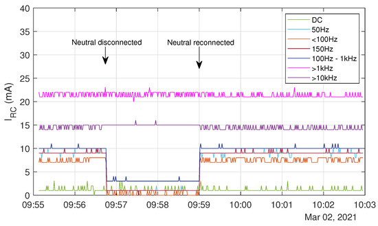
Figure 12.
Experimental results of scenario 3: Behaviour of the residual current in combination with an immediately disconnected neutral line N.
3.1.5. Scenario 5: DC Electric Arcs
An arc in the DC circuit generally causes measurable high frequency parts over the whole observed bandwidth, as shown in Figure 13 and Figure 14. In this experiment, arcs with different load currents have been produced using the setup described in Figure 7. The level of the nominal current does not seem to have a visual effect on the residual current at all. Since this is a DC-based setup, the DC part of the residual current is faded out.
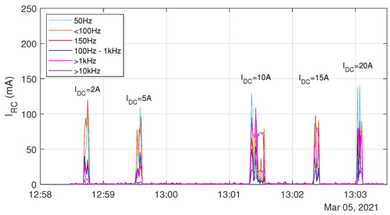
Figure 13.
Experimental results of scenario 5: Behaviour of the residual current influenced by manually produced arcs in a DC circuit.
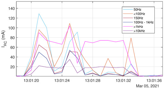
Figure 14.
Experimental results of scenario 5: Detailed view of the residual current in combination with a manually produced arc at a load current .
3.1.6. Summary
Table 5 provides an overview about the subjectively perceived behaviour of the residual current under the influence of the physically emulated faults.
Table 5.
Summary of the subjectively perceived effects of specific faults on the residual current separated into frequency parts. 1: Influenced by sensor effects; 2: For ground potential PE; 3: For neutral line N.
3.2. Fault Detection
3.2.1. Training Phase
Figure 15 shows the residual current (Figure 15a) depending on a DC power timeseries (Figure 15b) used as input data for the PV simulator to achieve a realistic infeed behaviour of the DUT. The timeseries is based on infeed data measured at a PV plant located at the DLR Institute of Networked Energy Systems. For the tests, two days have been chosen representing a cloudy and a sunny day. The datasets of both days have been combined and aggregated to one single curve with a length of ≈7 h.
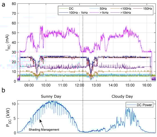
Figure 15.
(a): Residual current on the AC side of a PV inverter depending on a typical DC input power timeseries. (b): DC Input power timeseries as input data for the PV simulator based on combined and aggregated infeed measurements. The first half of the curve represents a sunny day, while the second half represents a cloudy day.
The algorithm has been trained using this dataset for two days to learn the systems normal behaviour. During the training phase, all control algorithms of the DUT were activated. One effect that can be seen in these curves is the shading management algorithm, a common method to handle module shading. In this case, the inverter starts passing through the whole PV curve every 5–6 min to detect whether there are local MPPs beside the global MPP with the highest DC power, a phenomenon that is typical for partly shaded PV modules. In the residual current, this algorithm has the highest impact in the upper frequency ranges . Although there is no direct correlation between the residual current and the input power visible, the residual current has a high fluctuation especially in the frequency range due to the input power changes. At approx. 09:30 and 12:45, the residual current drops throughout the whole frequency bandwidth except and DC.
After the two-day training phase, some fault scenarios were reproduced under normal operating load. The purpose of these experiments is to investigate the ability to detect injected faults under normal operating conditions. A selection of three important scenarios is discussed in the following sections. For each scenario the resulting residual current compared to the reconstruction error given by the state estimation algorithm and the anomaly factor given by the anomaly factor algorithm is shown.
3.2.2. Scenario 1: Instantaneous Increase of the Capacitive Resistance
The basic setup of the experiment is described in Section 2.6.1. As can be seen in Figure 16, the absolute value of the residual current does not increase significantly compared to the experiments from phase 1 (Section 3.1.1). This can be explained by the fact that in this experiment the inverter is operated under realistic operating conditions and thus the operational leakage current is generally increased compared to the experiments of the first phase. On the other hand, both the reconstruction error and the anomaly factor show increased values during the fault emulation. The highest reconstruction error with ≈700 is recorded at a capacity value of . For the anomaly factor, the dominant frequency ranges are below .
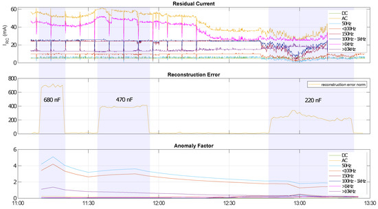
Figure 16.
Analysis results of scenario 1: Instantaneous increase of the capacitive resistance by adding capacitors ( at 11:10, at 11:35 and at 12:48) between line and ground.
3.2.3. Scenario 2b: Gradually Decrease of the Ohmic Resistance
The basic setup of the experiment is described in Section 2.6.3. As can be seen in Figure 17, a slow change in resistance does not result in a visible increase in residual current in this experiment either. The reconstruction error increases with decreasing resistance up to a value ≈22,000. With constant resistance, the reconstruction error remains at ≈15,000. As the resistance increases, the reconstruction error drops back to the initial value. The anomaly factor shows a similar behaviour and increases in the frequency range < with decreasing resistance up to a value of ≈140 (for the frequency range ).
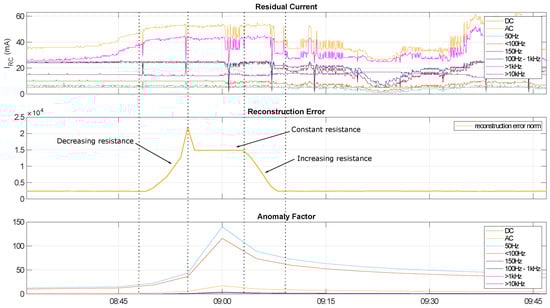
Figure 17.
Analysis results of scenario 2b: Gradually decreasing (starting at approx. 8:50) respectively increasing (starting at 9:05) resistive load between line and ground.
3.2.4. Scenario 3: Increased Series Resistances and Broken Lines
The basic setup of the experiment is described in Section 2.6.4. As can be seen in Figure 18, a line interruption leads to an immediate drop in the residual current. It is noteworthy that in this experiment mainly the ranges are affected, while in the experiments of the first phase (Section 3.1.4) mainly the low-frequency range was affected. The reconstruction error shows a small increase from 10 to 40 during the interruption, while the anomaly factor records no significant change.
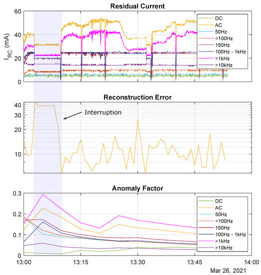
Figure 18.
Analysis results of scenario 3: Interruption of the neutral line N.
4. Conclusions
The goal of this project was a feasibility analysis that provides information about the possibility to detect and identify faults in inverter based energy systems using two machine learning approaches (pattern recognition and variational autoencoder) as a further stage of modern smart residual current monitors.
Experiments have shown that specific faults in an inverter based energy system have a significant impact on the residual current over a broad frequency range. Each of the fault emulations chosen for these tests produces a unique fingerprint that makes it certainly possible to detect and identify those faults using machine learning based algorithms. Another aspect that has been found was that the change of the input power as well as other outside influences, such as control algorithms, also affect the residual current. One of the main challenges at that point is the separation of those regular leakage currents caused by the interferences from the fault currents which are caused by faults. An algorithm has to be well trained to learn the system’s normal behaviour considering the whole bandwidth of possible system states.
Regarding the DCTR sensors, the switching of measuring ranges and as a consequence the change of the resolution also causes different measurement values that are not a result of faults and that could be misinterpreted. This effect has to be considered when designing a hardware sensor for this purpose.
Compared to conventional threshold-based methods, which are responsive to absolute changes of the residual current, the described approach basically allows for recognizing faults that obviously do not affect the total RMS value of the residual current. Physically emulated faults under nearly realistic conditions have shown that the reconstruction error and/or the anomaly factor detect these faults, while the absolute value of the residual current often does not show any significant changes despite the fluctuations caused by outside influences. It has to be considered that the experiments described in this article are performed using a laboratory setup that does not reflect the all-embracing behaviour of a grid-connected PV system. It is to be expected that in real PV plants, small signal levels especially are not that easy to detect since the Signal-to-Noise Ratio (SNR) is higher due to the outside influences from the grid and the behaviour of the inverter. Therefore, it is necessary to perform more investigations in real PV plants to improve the signal processing and to optimize the algorithm.
Author Contributions
Conceptualization, S.G. and H.B.; methodology, D.M. and A.J.; experiments, H.B.; result discussion, W.W.-S. and H.B.; project administration, H.B.; writing—original draft preparation, H.B.; writing—review and editing, G.R. and S.G.; writing—introduction, G.R.; funding acquisition, S.G. All authors have read and agreed to the published version of the manuscript.
Funding
This research received no external funding.
Institutional Review Board Statement
Not applicable.
Informed Consent Statement
Not applicable.
Acknowledgments
The authors would like to thank Moiz from the DLR Institute of Networked Energy Systems for his help preparing the laboratory experiments.
Conflicts of Interest
The authors declare no conflict of interest.
Abbreviations
The following abbreviations are used in this manuscript:
| MDPI | Multidisciplinary Digital Publishing Institute |
| DOAJ | Directory of open access journals |
| PV | Photovoltaic |
| DC | Direct Current |
| RMS | Root Mean Square |
| DUT | Device Under Test |
| MPP | Maximum Power Point |
| PoE | Power-over-Ethernet |
| RCM | Residual Current Monitor |
| RCD | Residual Current Device |
References
- DKE. DIN VDE 0100—200: Errichten von Niederspannungsanlagen; VDE Verlag: Berlin, Germany, 2006. [Google Scholar]
- Avizienis, A.; Laprie, J.C.; Randell, B. Fundamental Concepts of Dependability; Technical Report; Department of Computing Science Technical Report Series; 2001; Available online: https://eprints.ncl.ac.uk/file_store/production/55707/35D90208-2D34-4C19-BFB5-65E037791AE6.pdf (accessed on 22 July 2021).
- Stylianos, S.; Karolidis, D.; Voyiatzis, I.; Samarakou, M. Photovoltaic Faults: A comparative overview of detection and identification methods. In Proceedings of the 10th International Conference on Modern Circuits and Systems Technologies (MOCAST), Thessaloniki, Greece, 5–7 July 2021. [Google Scholar]
- Kumaradurai, A.; Coosemans, T.; Teekamaran, Y.; Messagie, M. Fault Detection in Photovoltaic Systems Using Machine Learning Algorithms: A Review. In Proceedings of the 8th International Conference on Orange Technology (ICOT), Daegu, Korea, 18–21 December 2020. [Google Scholar]
- Fazai, R.; Mansouri, M.; Abodayeh, K.; Trabelsi, M.; Nounou, H.; Nounou, M. Machine Learning-Based Statistical Hypothesis Testing for Fault Detection. In Proceedings of the 4th Conference on Control and Fault Tolerant Systems (SysTol), Casablanca, Morocco, 18–20 September 2019. [Google Scholar]
- Attouri, K.; Hajji, M.; Mansouri, M.; Harkat, M.; Kouadri, A.; Nounou, H.; Nounou, M. Fault detection in photovoltaic systems using machine learning technique. In Proceedings of the 17th International Multi-Conference on Systems, Signals and Devices (SSD), Monastir, Tunisia, 20–23 July 2020. [Google Scholar]
- Hajji, M.; Harkat, M.; Kouadri, A.; Abodayeh, K.; Mansouri, M.; Nounou, H.; Nounou, M. Multivariate feature extraction based supervised machine learning for fault detection and diagnosis in photovoltaic systems. Eur. J. Control 2021, 59, 313–321. [Google Scholar] [CrossRef]
- Bengio, Y.; Courville, A.; Vincent, P. Representation Learning: A Review and New Perspectives. IEEE Trans. Pattern Anal. Mach. Intell. 2013, 35, 1798–1828. [Google Scholar] [CrossRef] [PubMed]
- Ridgeway, K. A Survey of Inductive Biases for Factorial Representation-Learning. arXiv 2016, arXiv:cs.LG/1612.05299. [Google Scholar]
- Tipping, M.E.; Bishop, C.M. Probabilistic principal component analysis. J. R. Stat. Soc. Ser. (Stat. Methodol.) 1999, 61, 611–622. [Google Scholar] [CrossRef]
- Rumelhart, D.E.; Hinton, G.E.; Williams, R.J. Learning Internal Representations by Error Propagation. In Parallel Distributed Processing: Explorations in the Microstructure of Cognition, Volume 1: Foundations; MIT Press: Cambridge, MA, USA, 1986; pp. 318–362. [Google Scholar]
- Kingma, D.P.; Welling, M. Auto-Encoding Variational Bayes. arXiv 2014, arXiv:stat.ML/1312.6114. [Google Scholar]
- Higgins, I.; Matthey, L.; Pal, A.; Burgess, C.P.; Glorot, X.; Botvinick, M.; Mohamed, S.; Lerchner, A. beta-VAE: Learning Basic Visual Concepts with a Constrained Variational Framework. In Proceedings of the ICLR 2017 Conference Submission, International Conference on Learning Representations, Toulon, France, 24–26 April 2017. [Google Scholar]
- Burgess, C.P.; Higgins, I.; Pal, A.; Matthey, L.; Watters, N.; Desjardins, G.; Lerchner, A. Understanding disentangling in β-VAE. arXiv 2018, arXiv:stat.ML/1804.03599. [Google Scholar]
- Datenblatt TC.ACS.30.528.4WR.S.LC. Available online: https://www.regatron.com/assets/resources/Documents/Technical-Datasheets/TC.ACS/DS_TC.ACS.30.528.4WR.S.LC_EN_210518.pdf (accessed on 24 August 2021).
- Datenblatt EA-PSI 91000-30 3U 19″ 3HE. Available online: https://elektroautomatik.com/shop/media/pdf/ef/a8/ee/datasheet_psi9000_3u.pdff (accessed on 24 August 2021).
- Datenblatt Differenzstrommonitore DCTR B-X Hz 035-PoE. Available online: https://www.doepke.de/uploads/tx_doepkeproducts/datenblatt/doepke_09344937_dbl_de.pdf (accessed on 24 August 2021).
Publisher’s Note: MDPI stays neutral with regard to jurisdictional claims in published maps and institutional affiliations. |
© 2022 by the authors. Licensee MDPI, Basel, Switzerland. This article is an open access article distributed under the terms and conditions of the Creative Commons Attribution (CC BY) license (https://creativecommons.org/licenses/by/4.0/).