Voltage-Based Load Recognition in Low Voltage Distribution Grids with Deep Learning

Abstract

Due to the increasing penetration of renewable energies in lower voltage level, there is a need to develop new control strategies to stabilize the grid voltage. For this, an approach using deep learning to recognize electric loads in voltage profiles is presented. This is based on the idea to classify loads in the local grid environment of an inverter’s grid connection point to provide information for adaptive control strategies. The proposed concept uses power profiles to systematically generate training data. During hyper-parameter optimizations, multi-layer perceptron (MLP) and convolutional neural networks (CNN) are trained, validated, and evaluated to determine the best task configurations. The approach is demonstrated on the example recognition of two electric vehicles. Finally, the influence of the distance in a test grid from the transformer and the active load to the measurement point, respectively, onto the recognition accuracy is investigated. A larger distance between the inverter and the transformer improved the recognition, while a larger distance between the inverter and active loads decreased the accuracy. The developed concept shows promising results in the simulation environment for adaptive voltage control.

1. Introduction

The share of renewable energies for gross power consumption in Germany rose to 45.4% in 2020 [1]. To achieve the climate targets defined in international and national agreements, the government plans to increase this share up to 65% in 2030 [2]. The associated decentralization of the power grid architecture with fluctuating feed-in leads to new requirements regarding a reliable power grid operation [3]. Due to the different characteristics of distributed energy resources (DERs) in comparison to conventional generators, a new way of providing ancillary services is necessary, especially in local voltage control [4]. Additionally, the number of loads and generating plants connected to the lower voltage level increased in the last couple of years and an ongoing increase in future can be expected [5]. For example, the government’s goal is a number of seven to ten million registered electric vehicles (EVs) in Germany in 2030 [2]. This expectation increases the challenge of grid voltage stabilization even more because every active grid participant affects the voltage and the variety of different grid scenarios caused by parallel activation of different loads and generators increases. The overarching goal of voltage control is to remain inside a tolerance band of $\pm 10$% of the nominal voltage [6]. To guarantee a stable voltage in the long term despite these developments on both sides of a grid connection point, there is a need for further development on using the abilities of power electronics and the inverters, which are the interfacing devices to the power grid for most of the DERs. Current approaches to achieve voltage stability were reviewed by Mahmud and Zahadi [7]. Some advanced methods for voltage control enable inverters to contribute to decentralized voltage control. Especially, there are different voltage control strategies with a fixed $cos\phi ,cos\phi \left(P\right)$, or $Q\left(U\right)$ [8]. Another approach is the usage of machine learning for reactive power control of inverters. For this, both centralized and decentralized approaches based on reinforcement learning were developed [9,10,11,12,13].

Moreover, the implementation of energy management systems and the scheduling and monitoring of active devices is another research field contributing to an increase in energy efficiency and grid stabilization. In this research field, the so called non-intrusive load monitoring (NILM) is a growing topic. It deals with the recognition of loads in households or industrial buildings by disaggregation of aggregated data acquired from a single point of measurement like smart meters and was founded by Hart [14]. The general idea of NILM is to exploit the repeated appliance of particular loads in a building profile and their associated, repeated patterns in the measurement data. An overview of different NILM approaches was given by Aladesanmi and Folly [15]. They listed techniques based on active and reactive power as well as voltage and current. Faustine et al. described event-based and state-based NILM algorithms, and they mentioned two different signatures to rely on: transient signatures, which were used by Ghosh et al. [16] and Athanasiadis et al. [17], and steady-state signatures [18]. In addition, as state-of-the-art algorithms regarding NILM, they described for example hidden Markov models and deep learning approaches using recurrent neural networks and convolutional neural networks [17,18]. Huber et al. reviewed the current status in Low-Frequency-NILM using deep learning and discussed aspects like neural network architectures, data input shape, and windowing the time series data [19]. Next to a variety of distinct electrical features for NILM, Bernard differentiated NILM tasks with deep learning in supervised and unsupervised learning, before he decided to develop an unsupervised learning technique to disaggregate the measured load profile of a household [20]. Furthermore, Brucke et al. proposed an unsupervised approach connecting to a forecast of load state changes [21]. Besides, Parson et al. combined a supervised approach for development of probabilistic models of appliances and an unsupervised approach to fine-tune these models by aggregated household data with the goal to overcome the challenge of unlabeled appliances [22]. However, Zufferey et al. successfully demonstrated a supervised learning approach using power, voltage, and current signatures of distinct loads to recognize electric loads based on their consumption profiles [23]. They developed stochastic models for appliance classes and used k-Nearest Neighbor algorithm and Gaussian mixture models. By de Souza et al., a supervised learning approach based on a detection machine was proposed to figure out when a load is turned on or off [24]. Another example for modeling the NILM task as a supervised learning setting was given by Basu et al., who presented a temporal multi-label classification using sliding windows, binary label vectors and different machine learning algorithms [25]. Also, Singh and Majumbdar formulated a multi-label classification task with a sparse representation approach based on the assumption that for every test sample there is a representation as a linear combination of training samples [26]. Furthermore, Ruzzelli et al. developed a concept for profiling appliances, building a training dataset, and learning a neural network to recognize the active appliances in real time [27].

Generally, in NILM the data are often acquired directly at the grid connection point of a building, so that the observing direction is from the grid connection point to the consumer or prosumer side to investigate the load behavior inside the building. In this paper, the idea is to invert this observing direction to analyze load behavior at surrounding grid connection points additionally. This means, the challenge for the proposed method is the online recognition of loads based on their characteristic voltage profiles, while their influence on the grid voltage measured at a particular grid connection point is affected by the size of the load, its grid position, the local grid topology, and also the total number of active loads. So, in a sense, the appearance of a load in the grid voltage depends on more grid properties than in NILM scenarios.

The author’s future vision is to develop a self-learning inverter, which independently analyzes the measured voltage data at the inverter’s grid connection point, recognizes patterns in the data, and derives the optimal control strategy for active and reactive power management to stabilize the power grid without additional information. The first step of this development is the analysis of the conditions inside the local grid environment experienced by an inverter. This leads to the following idea of this study, which provides a setting similar to NILM tasks, demonstrated with an example of two EVs. As mentioned above, the field of e-mobility will be expanded in the upcoming years, so that the number of EVs will increase [2]. The corresponding charging stations are usually installed in the low voltage level and the EVs have a significant impact on the voltage behavior in local grid environments as investigated by Dharmakeerthi et al. [28]. The intelligent inverter will measure the grid voltage. Because of the possible high demand in power during the charging process of EVs, the inverter will observe significant changes in the voltage signal. Over the course of time, an EV with a characteristic charging profile, which depends on the EV type, the charging status, the temperature, and the maximum charging power, will be charged at different times of the day, and it might even change the location for charging in the grid. Nevertheless, it can be assumed that every time it is charged, it will cause a similar voltage pattern. The inverter will learn and recognize this repeated pattern. Consequently, it will be able to adapt the feed-in of active and reactive power for its specific local grid environment. Thus, it will be able to derive the optimal control strategy to stabilize the grid based on the learned voltage patterns.

Therefore, in this paper, a method to classify particular load types in a local grid based on the voltage level observed at the inverter’s grid connection point is presented. The main contributions of this paper can be listed as follows:

(1)

The proposed method can be used in an online manner to recognize large loads in the local grid environment within a time range of a few hundreds of seconds while only using the measured voltage level. Instead of observing households, the surrounding grid environment can be analyzed and grid participants from other grid connection points can be recognized.

(2)

A concept how to generate a dataset to train a recognition algorithm without a need for extensive simulation effort is provided.

(3)

For demonstration, the developed method is applied to simplified grid situations with only two EVs charging in a test grid structure, which represents a proof of concept for this method.

(4)

It is shown that in low voltage distribution grids the relative location of the active loads, the transformer, and the inverter influences the load recognition accuracy in a significant manner.

(5)

The results of the investigations in this study indicate that in comparison to multi-layer perceptrons the convolutional neural networks are the better choice to use for load recognition in time series data.

This paper is organized as follows. In Section 2, the overall recognition approach is described in detail and it is presented how the recognition is optimized. This is followed by Section 3, where the recognition results of the example demonstration on two EVs are shown. In the second part of this section, the influence of different line lengths between transformer, inverter, and a load in a test grid is investigated. The results are discussed in Section 4, and this paper is concluded in Section 5.

2. Materials and Methods

2.1. General Concept

The overall goal of the methodology presented in this paper is the recognition of repeated voltage patterns. To achieve this, the recognition was considered as a (multi-dimensional) time series classification task. This means that based on the voltage data the states of selected load classes were identified.

On the one hand, a class could be defined as a single load, that is, the corresponding load profile should be detected in the voltage signal. On the other hand, a class could be seen as the load type, so that a couple of load profiles could be categorized in the same way.

Mathematically expressed, the task can be formulated as following:

2.1.1. General Task Formulation

Let ${\mathbb{X}}^m$ be the m-dimensional feature space. This means, there are m different variables measured or computed. The input of the classification algorithm would be a continuously provided time series $S={\left(s_t\right)}_{t\in \mathbb{T}}$ with $s_t\in \mathbb{X}$ and $\mathbb{T}$ representing a 1 s-resolution for data acquisition.

To train the classification algorithm, the multi-dimensional time series is cut with a sliding window approach as used by Krystalakos et al. [29]. In this approach, a window length n is defined. This window is shifted along the time series using a step-size of 1 s, and each of the shifted windows with the last n data points is used as one sample. Then, a window w at time $t_0$ has the form $w_t:={(s_{t_0},s_{t_0-1},\dots ,s_{t_0-n+1})}^T$.

The output of the algorithm is desired as a binary status of every class. This means, the output vector’s dimension is defined as the number of trained classes, which is denoted by c. The entries of this vector are equal to 1, if the corresponding class is active, or equal to 0, if not. The corresponding binary vectors representing the class states are used as labels to formulate the whole task as a supervised learning problem.

Therefore, the desired classification mapping is

$$f:{\mathbb{X}}^n\to {\mathbb{B}}^c\mathrm{with}{w}_t\to \left(\begin{array}{c}{b}_1\\ ⋮\\ b_c\end{array}\right).$$

(1)

This type of formulation of a classification task refers to so called multi-label classification. It was also used in other applications like image classification [30,31,32] and in the field of NILM by Basu et al. [25], Singh and Majumbdar [26], and by Massidda et al. [33].

Because of the vision of a standalone inverter, which should be able to adjust the active and reactive power management in terms of repetitive load profiles of electrical loads in its grid environment, the recognition concept was based only on data measured at the grid connection point. In detail, the voltage values from the three phases of the power grid were used as root-mean-squared values in 1 s-resolution, related to the nominal voltage (per unit specification). This setting was chosen under the assumption that loads do not change their status (active or inactive) within one second more often than once. Additionally, the voltage harmonics caused by activation of a load at other grid connection points than the measurement point are not recognizable over that distance. If only symmetric loads are active, the voltage is very similar for each grid phase. Nevertheless, it was useful to include all three phases in the input data generated in this concept because there are asymmetric loads. The classification algorithm received not only the raw measured voltage values as an input, but also computed data as kind of a derivative. In detail, it was the difference of the current value ($t=0$) to the value one time-step before ($t=-1$). The idea for this additional feature was to avoid a recognition only based on absolute values, which could easily lead to an incorrect classification of voltage patterns with slightly different magnitudes.

In total, this led to the special case of $m=6$ in Equation (1) as follows.

2.1.2. Example Task Formulation

Let ${\mathbb{X}}^6$ be the six-dimensional feature space and S be a multi-dimensional time series, while $c=2$ is the number of trained classes and n is the window length. The variable $v_{Li,t}$ denotes the voltage at time t from grid phase $i=1,\dots ,3$ and $d_{Li,t}:=v_{Li,t}-v_{Li,t-1}$ represents the difference between the voltage values from time t and $t-1$ on grid phase i. Furthermore, let $s_t\in S$ be the data point at time t with $s_t=(v_{L1,t},d_{L1,t},v_{L2,t},d_{L2,t},v_{L3,t},d_{L3,t})$. Then, one sample at time $t_0$ has the form $w_{t_0}:={(s_{t_0},s_{t_0-1},\dots ,s_{t_0-n+1})}^T$.

Finally, the classification task is to find a mapping

$$f:{\mathbb{X}}^{n\times 6}\to {\mathbb{B}}^2\mathrm{with}{w}_t\to \left(\begin{array}{c}{b}_1\\ b_2\end{array}\right).$$

(2)

For the classification machine learning was applied. This was reasoned by the repeated voltage patterns and the many complex pattern recognition problems machine learning could already solve successfully, e.g., in fields of image classification [34,35,36], face recognition [37], speech recognition [38,39], games [40], and various time series classification applications [41].

In this use case, the algorithm had to learn the underlying relation of voltage drops in power lines and the activation of particular loads causing power flow through the lines. The corresponding formula for voltage drop calculation in a power grid is

$$\Delta V=\sqrt{3}·L·I·cos\left(\phi \right)·\frac{1}{\kappa ·q}$$

(3)

with voltage V, line length L, current I, power factor $cos\left(\phi \right)$, specific conductance $\kappa$ and conductor cross-section q [42].

Because the overall goal is to achieve a stable power grid, some knowledge about loads which are active in the local grid environment around an inverter would be helpful to be able to derive an optimal control of active and reactive power feed-in. Therefore, in the recognition phase it is necessary to have a clear assignment to a class of loads. By this requirement, unsupervised learning approaches like mentioned in the introduction regarding the field of NILM were excluded (e.g., [20]).

2.2. Algorithm Selection

If this concept would be applied in a real power grid, there would be a huge number of active loads, load types, and trainable classes, so that the classification task would be very complex. Furthermore, a situation would be conceivable in which the trained algorithm should be extended to a new load class, so the output vector’s length would be increased. From these future challenges regarding a high complexity and a possible extensibility, it can be concluded that artificial neural networks are assessed as a good choice to use for the underlying problem.

In this paper, two popular architectures of neural networks were investigated.

2.2.1. Multi-Layer Perceptron Neural Network (MLP)

A multi-layer perceptron network consists of an input layer, some hidden fully connected layers, and an output layer. In a classification setting, the input layer gets an input vector of a previously specified length and processes the input. The results are passed to the next hidden layer. Here, in each unit (neuron) of the layer a weighted sum is computed. This sum is used as an input for a (non-linear) activation function and the returned value is given to the neurons of the next layer. At the end, a single output layer returns the overall output of the neural network. Depending on the structure of the task to be solved, this layer consists of as many neurons as classes considered in training. Furthermore, depending on the kind of implementation, e.g., the output is a vector containing values between zero and one. These can be interpreted as the confidence of the MLP to classify the input into the corresponding class. For example, these values can be rounded to get the desired binary output vector.

The MLP architecture was tested in the course of this paper because it is the simplest neural network architecture.

2.2.2. Convolutional Neural Network (CNN)

A convolutional neural network generally consists of an input layer, a sequence of convolutional and pooling layers, a sequence of fully-connected layers, and an output layer. Applied to the time series classification setting, the input layer gets a matrix representing a section of the multi-dimensional time series. In a convolutional layer a specified number of filters with predefined sizes (kernel size) is shifted over the layer’s input and discrete convolutions are computed. The results are forwarded to a pooling layer, in which a down-sampling method for dimensionality reduction is applied. At the end of the architecture, a variable number of fully-connected layers as in MLPs is used and the output is returned as a vector of values between 0 and 1 as the output layer of an MLP provides it. As for MLPs, a rounding step can be implemented to get the desired binary output vector.

This type of a neural network is often used in image applications because it is very powerful in pattern recognition, e.g., [34,37]. In Keras API, there is also an adapted version of convolutional layers called $Conv1D$ available [43]. This version is offered especially for usage of convolutional layers in time series applications and uses filters shifted only in the time direction instead of two directions as in image applications.

2.3. Training Environment

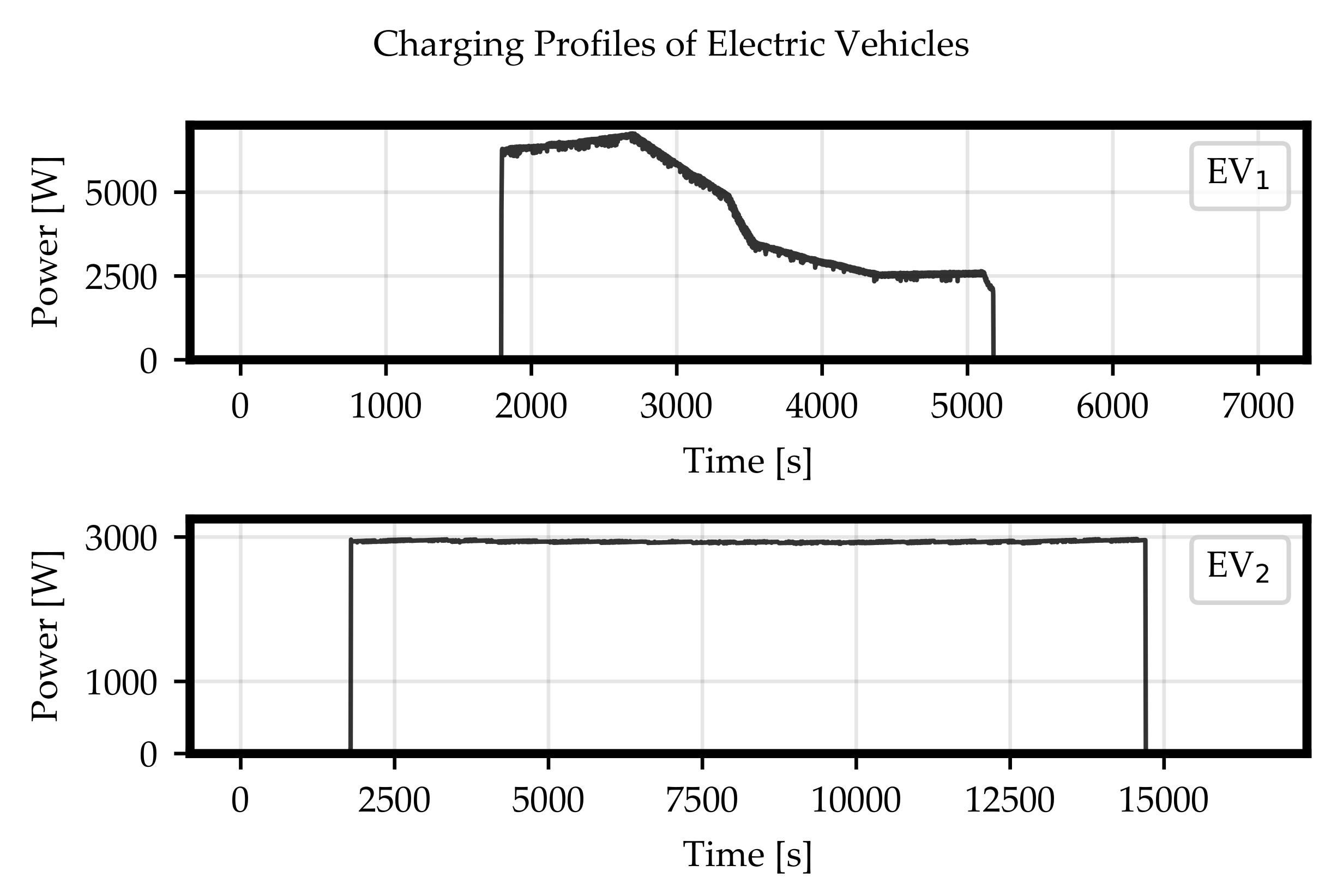
To solve the described multi-label time series classification task with neural networks, the weights had to be trained, and therefore a training dataset was needed. This dataset had to represent the possible scenarios a classification algorithm could face in the real application. In this paper, the task was simplified to just two EVs (see Figure 1) symmetrically charging in a reference grid (see Figure 2), such that the considered classes were represented by these EVs ($c=2$).

The procedure to generate a suitable training dataset is described in the following paragraphs.

2.3.1. Phase 1—Power Profiles

The first step of dataset generation is the power profile collection of the load classes to be recognized. For this, data sheets or laboratory measurements can be considered. This step is optional because the algorithm is trained on voltage data, not power values. This means, Phase 1 can be skipped if appropriate voltage data are already available.

For this paper, two active power profiles measured in 1 s-resolution located at two charging stations at the DLR were used (see Figure 1). The corresponding measurement devices offered a resolution of around ${10}^{-5}$ V. Because of this, the entire simulated data used in this paper were rounded to this resolution [44].

2.3.2. Phase 2—Voltage Profiles

The second step dealt with the simulation of the corresponding voltage profiles belonging to the desired load classes. So, a grid structure was needed to simulate the grid behavior during active periods of these classes.

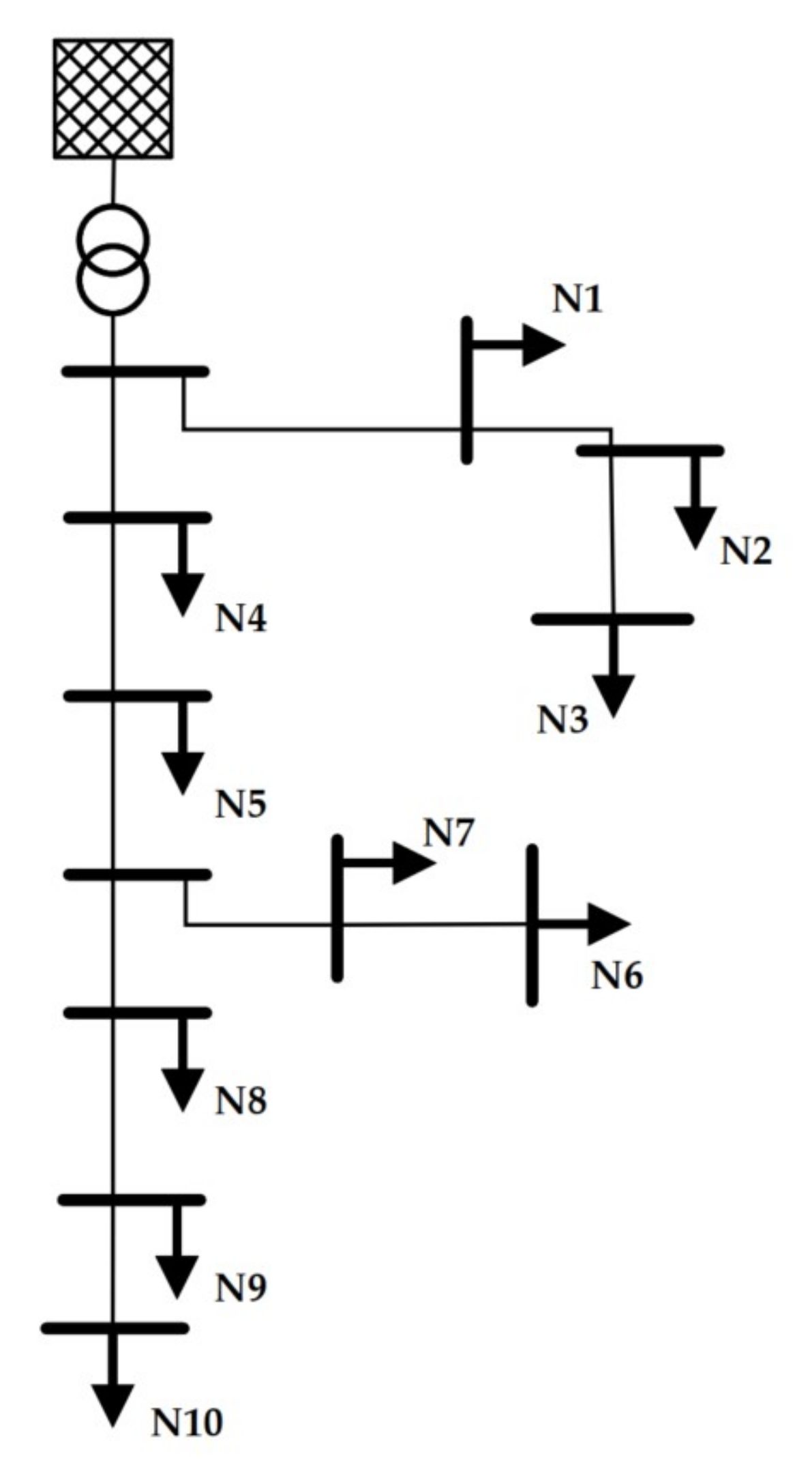
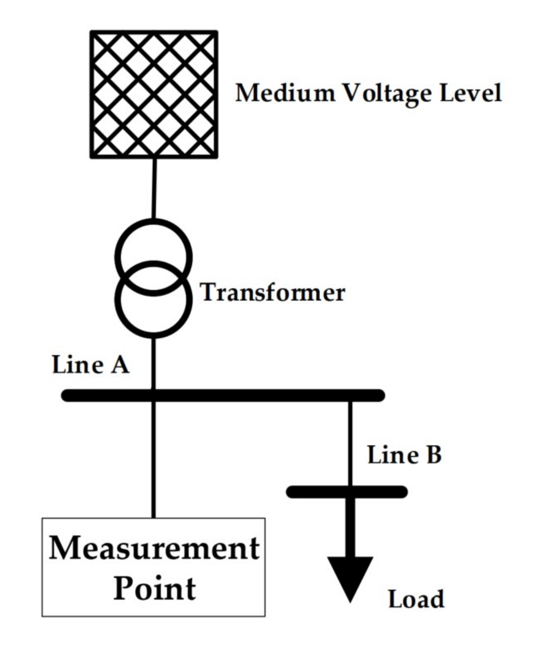
For this, a power grid model was built in MATLAB/Simulink (Release 2020b), presented in Figure 2. As the model was a three-phase–21-bus system developed in the Merit Order Netzausbau 2030 (MONA) project, it represented a European low voltage distribution grid with ten possible grid connection points operating at nominal grid frequency of 50 Hz and 400 V as nominal voltage [45]. At each grid connection point one Three-Phase Dynamic Load block from the MATLAB toolbox Simscape (add-on Simscape Electrical) was connected [46,47]. This block allows the external control by an array of active and reactive power values. The power grid lines were represented by Three-Phase PI section line-blocks, in which parameters for line length, resistance, inductance, and capacitance can be defined. The simulation data consisted of three-phase root-mean-square-values scaled by the nominal voltage (per unit, in short pu) in 1 s-resolution. This data were measured at one grid node ($N10$) representing the grid connection point of an inverter. The data were stored in a SQL-database and exported to csv-files.

Figure 2. Scheme of reference grid number 8 from [45] with labeled grid nodes.

Figure 2. Scheme of reference grid number 8 from [45] with labeled grid nodes.

This model built in MATLAB Simscape can be perfectly used as a validated environment for the machine learning algorithm because the simulation software is commercially provided, the implemented grid topology was developed in a scientific project, and the overall functionality was continuously tested during implementation.

2.3.3. Phase 3—Training Data Generation for Different Grid Connection Points

It is necessary to include the activation of each considered load type at different grid connection points because different locations affect the size of the voltage drops in the profiles. At first, the voltage profiles corresponding to both classes without influence of other grid participants were simulated through external control of one load block at grid node $N10$ in the grid model. After this, these profiles were scaled between the allowed voltage limits of 0.9 pu and 1.0 pu with scaling factors equally distributed between 0 and 1 to cover the tolerance band and thus the possible occurring voltage values. In the example of two EVs only five different scaling factors were used to generate five scaled voltage profiles (see Figure 1) but this number could be adapted to the higher complexity of further investigations. This phase ended with the computation of the corresponding difference feature.

2.3.4. Phase 4—Training Data Generation for Overlapping Periods

It is possible that the trained classes have overlapping active periods. If one profile is shifted along the other, every 1 s-shift means a new activation scenario because the resulting voltage pattern can look significantly different. Therefore, the simulation effort would be immense. So, the huge number of different combinations for this scenario could not be simulated. However, the challenge of limited computer capacities can be solved by the training of neural networks with a reduced number of different overlapping combinations to get a model which is able to generalize the behavior of both classes. For this, one profile was held, while the other one was shifted along it in regular steps, and vice versa. This phase was completed by the computation of the difference feature.

Besides, the neural network has to learn the undisturbed look of the power grid. If the dataset would only consist of samples with labels including an entry equal to 1, the neural network would not be able to learn that the vector ${(0,0)}^T$ is a possible output. Because of this, there were periods with no activation of loads included. All the described single datasets were appended to create a large dataset representing the expected different grid scenarios.

2.3.5. Phase 5—Training Phase

Before training, the corresponding data were preprocessed. More precisely, both features were scaled by

$$\widehat{x}:=\frac{x-x_{min}}{x_{max}-x_{min}},$$

(4)

whereas $x\in \mathbb{R}$ represents the particular feature value $v_{Li,t}$ or $d_{Li,t}$, respectively, (see Section 2.1, Equation (2)). The interval $[x_{min},x_{max}]$ represents the range in which the respective feature values are expected.

The presented load recognition method was applied to two different EVs, which are charged at different grid connection points in the reference grid. This implies that the case of generation plants was not considered. Therefore, the grid voltage was limited upwards to $x_{max}=1.0$. The lower limit for voltage scaling should be $x_{min}=0.9$ due to the voltage tolerance band on low voltage level of $\pm 10$%. The difference values were scaled based on $x_{min}=-0.003$ and $x_{max}=0.003$.

The neural networks in this paper were implemented with Keras API [43], based on Tensorflow (Version 2.4.0) [48]. These models were trained by the fit method from Keras in an offline supervised learning setting. This means, the whole training data were collected and labeled before training.

As mentioned in Section 2.2, the neural networks return vectors from ${\mathbb{R}}_{0\le 1}^c$. For this reason, a rounding step was executed to evaluate the final training results. Within the fit method of Keras a binary cross-entropy function was used to calculate the losses during training and a maximum number of 100 epochs was set. This number might be not completely utilized because the training could be stopped earlier by an Early-stopping-callback function provided by Keras.

Following the described procedure, a final multi-dimensional time series of 239,948 s was obtained. With two classes ($c=2$) to train, there were $2^2=4$ possible combinations which had to be included in the dataset. These are presented in detail in

Table 1. Composition of the dataset for training in this paper (0 for inactive, 1 for active).

Step	Class 1	Class 2	Training
1	1	0	Scaling factors:
			0.92, 0.94, 0.96, 0.98, 1.0
			31,268 samples ≈ 13.0%
2	0	1	Scaling factors:
			0.92, 0.94, 0.96, 0.98, 1.0
			174,173 samples ≈ 72.6%
3	1	1	Number of shifts with fixed EV${}_1$: 5
			Number of shifts with fixed EV${}_2$: 5
			19,507 samples ≈ 8.1%
4	0	0	In final dataset:
			15,000 samples ≈ 6.3%

.

The dataset is balanced in that both EVs are activated five times while the other one was inactive. The different shares of the samples were caused by the different lengths of the load profiles. However, despite these differences the neural networks could be successfully trained, as shown in the results section.

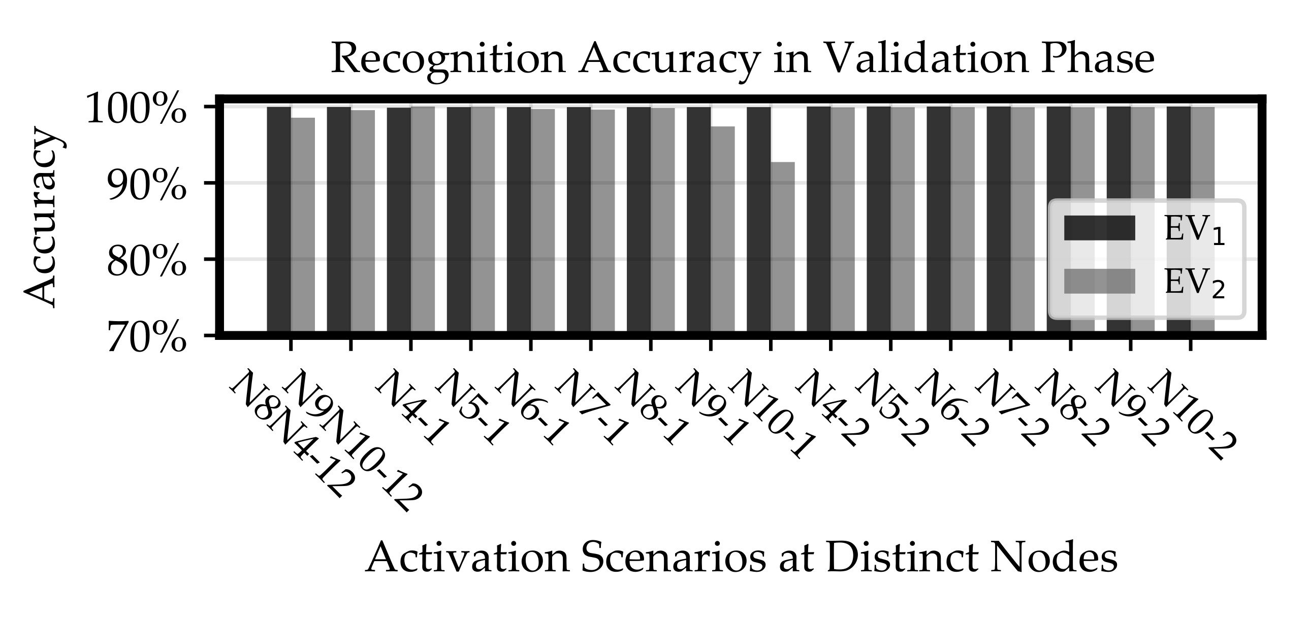
2.4. Validation

In the validation phase, it was tested whether a trained neural network was able to recognize the status of both EVs correctly, during activation of a single EV and also in parallel activation. The corresponding activation scenarios were simulated in the grid model described in Section 2.3, whereby the possibility of charging at different grid connection point and overlapping scenarios was taken into account (Phases 3 and 4). For these, the voltage was measured at node $N10$ because it is the grid connection point which is farthest away from the transformer. This point was chosen because the voltage fluctuations from all previous nodes have a direct influence on $N10$ in particular. How strong these fluctuations at $N10$ are depends on the cable lengths between the load and the transformer. The greater the line length, the greater the fluctuation. For this reason, nodes which are far away from the transformer are particularly exposed to strong voltage fluctuations and load recognition is essential to compensate voltage band violations.

For Phase 3, the activation of each type of load was simulated at nodes $N4$–$N10$. The remaining nodes $N1$–$N3$ are the nearest to the transformer and the farthest to the measurement point. From a real application perspective, it is more desirable to have an accurate performance in the near environment of an inverter’s grid connection point than far away from that node because the closer loads have higher impact to the voltage at the specific node. So, it has to be avoided that a neural network is optimized such that the classification accuracy is increased at grid nodes $N1$–$N3$, while the accuracy might drop for the other grid nodes. This was achieved by omission of scenarios at nodes $N1$–$N3$.

Each considered node yielded a single time series for each trained class: In the first half no load was active and in the second one the specific load was activated. By this, it was possible to validate the steps 1, 2, and 4 from Table 1.

Besides for Phase 4, some datasets were needed to investigate the ability of the neural network to recognize the class states during overlapping scenarios (Table 1, step 3). With this goal, one scenario for a charging process of EV${}_1$ at node $N8$ and one of EV${}_2$ at node $N4$ was simulated. Another dataset contained the measured values from a simulation with EV${}_1$ charged at node $N9$ and EV${}_2$ active at node $N10$. The shifts were randomly computed as 7453 s and 2335 s, respectively. These two overlapping scenarios were chosen under consideration of the grid section used in validation. The first one represents the activation of EV${}_1$ close to the measurement point while EV${}_2$ was located at the farthest node considered in validation. By this setting, it could be tested whether a neural network is able to separate a pattern from a far node and a pattern caused at a close node. In contrary, the second scenario consists of an EV${}_2$ closer to the measurement point than EV${}_1$. With this scenario, it could also be validated whether two patterns generated close to each other can be separated by the trained classifier. Because of the specific form of the EV${}_2$’s pattern similar to a rectangle, it has been decided to use just a single shift per location setting of both EVs.

This procedure led to 7 + 7 + 2 = 16 scenarios for validation. After simulation, the entire data were preprocessed in the same way as described in Section 2.3, Phase 5. Then, the trained neural network was used to run a classification for each single dataset k.

2.5. Evaluation

When a neural network is used to classify the validation data, a metric is necessary to evaluate the classification performance and to be able to compare the results of different neural networks.

This metric had to include a recognition accuracy of all classes. Besides, it should be considered that the neural network was required to have correct classifications for active, inactive and overlapping times for all classes. Because of this, the accuracies based on all correctly classified samples were used in Equation (5). By the product term, a neural network was penalized if it focused on just learning one class, while others were ignored. The maximum value was only reachable if a neural network was able to classify both classes in a right way.

With $c=2$ in the focused case of this paper, the formula for the accuracy corresponding to a single dataset k was

$$Ac{c}_k:=Ac{c}_{k,E{V}_1}+Ac{c}_{k,E{V}_2}+Ac{c}_{k,E{V}_1}·Ac{c}_{k,E{V}_2},$$

(5)

with $Ac{c}_{k,E{V}_i}:=\frac{T{N}_{k,i}+T{P}_{k,i}}{N_k}$, where $N_k$ was the total number of samples of dataset k. Further, $T{N}_{k,i}$ denoted the number of true negatives for class i, which is the number of samples correctly classified as inactive, and $T{P}_{k,i}$ was the number of true positives for class i, which is analogously the number of samples correctly classified as active.

The final score for the total validation had to be balanced for the two cases where just one EV is activated and the overlapping case. This was achieved by computation of a weighted sum with equal sums of weights for these three categories and equal weights within the categories:

$$Scor{e}_{final}:=\sum _{k=1}^{16}{w}_k·Ac{c}_k$$

(6)

with weights $w_k$ satisfying ${\sum }_{k=1}^{16}{w}_k=1$ and $w_k\ge 0$, $k=1,\dots ,16$. While the datasets for overlapping cases were associated with $k=1,2$, it was required that

$$\begin{array}{c}\hfill \begin{array}{ccccc}{w}_1=w_2,& w_3=\dots =w_9,& \mathrm{and}\hfill & w_{10}=\dots =w_{16},& \hfill \mathrm{with}\\ w_1+w_2=\frac{1}{3},& \sum _{k=3}^9{w}_k=\frac{1}{3},& \mathrm{and}\hfill & \sum _{k=10}^{16}{w}_k=\frac{1}{3}.\end{array}\end{array}$$

Obviously, it was $Ac{c}_k\in [0,3]$. Therefore, the highest achievable score for the neural network in validation phase is

$$Scor{e}_{final}=\sum _{k=1}^{16}{w}_k·Ac{c}_k\le 3·\sum _{k=1}^{16}{w}_k=3.$$

(7)

2.6. Hyper-Parameter Optimization

The pattern recognition is significantly influenced by the configuration of the neural networks, the preparation of load profiles and simulated data from grid models, and by the design of the training process. The improvement of the related, non-trainable parameters refers to hyper-parameter optimization. For this investigation, the Optuna version 2.4.0 was used, which offers a framework to optimize the user-defined hyper-parameters [49].

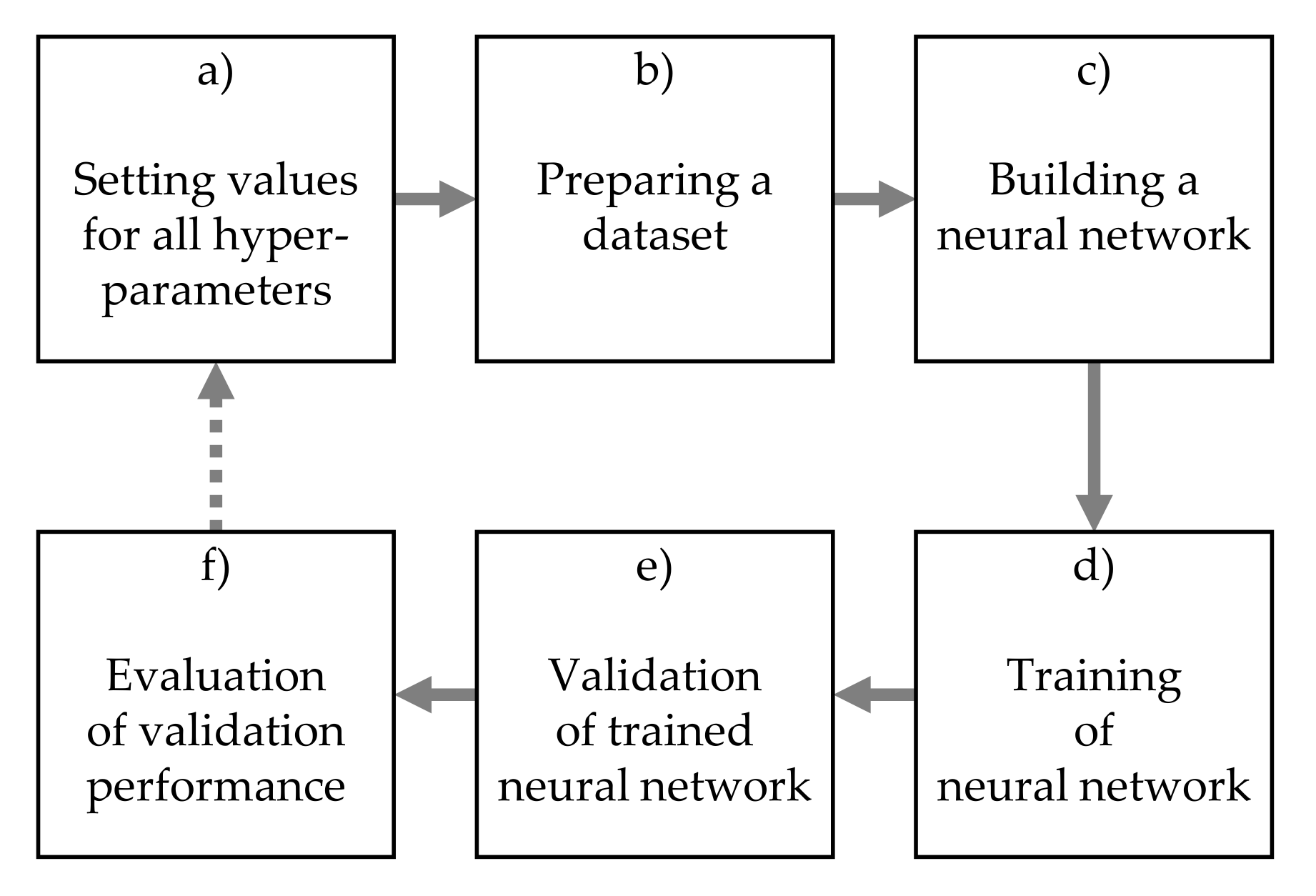
Each hyper-parameter optimization step from the proposed concept consisted of the sub-steps shown in Figure 3:

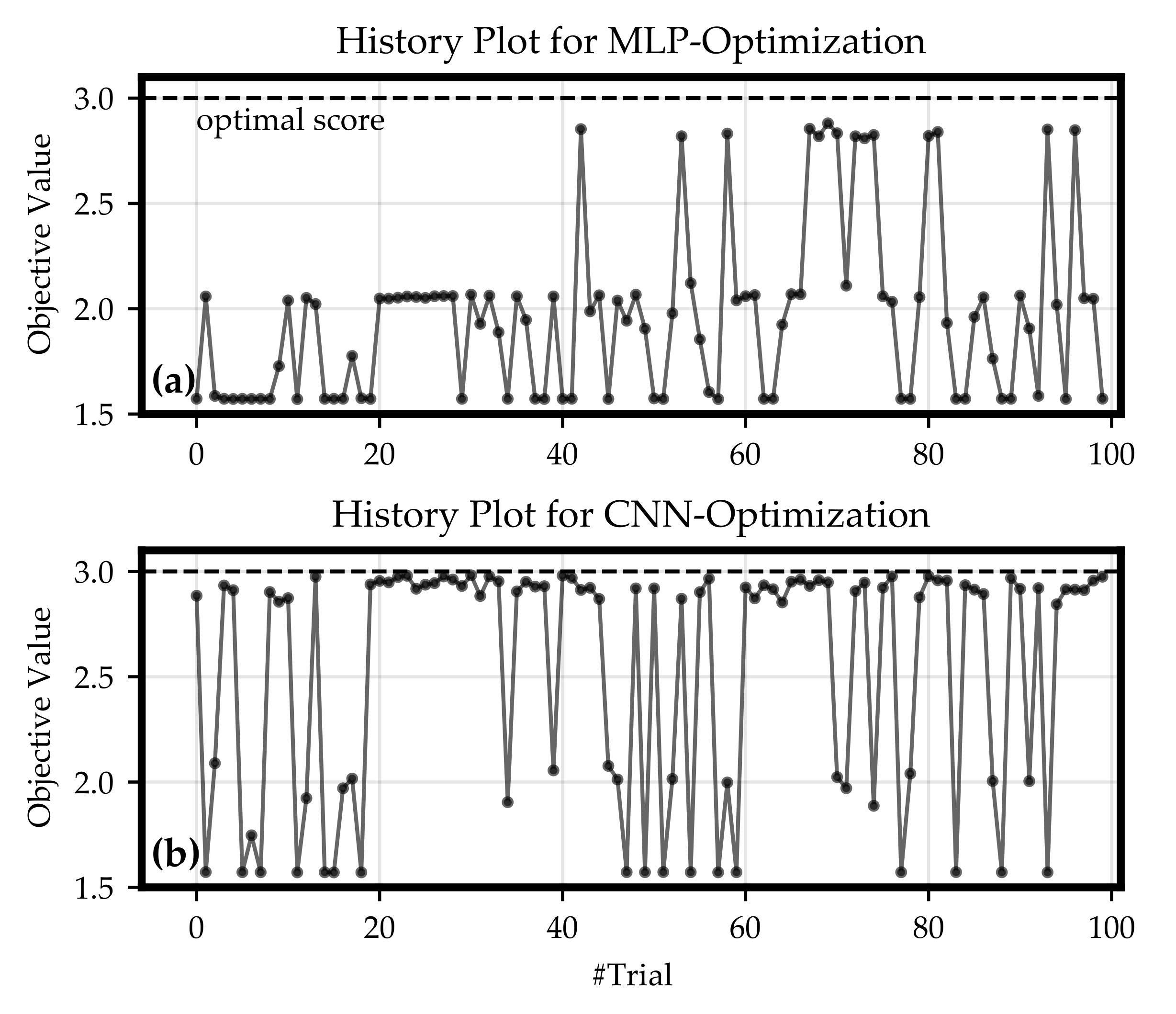
At the end of such a step an objective value was calculated by a custom objective function. In this paper, the objective value was chosen as the score in Equation (6). Based on this objective value, a tree-structured parzen estimator (TPE) algorithm was used to find the best configuration in the defined hyper-parameter space. The TPE is a sequential model-based optimization approach. For each optimization step, a trial is defined by setting a value for each hyper-parameter. To calculate these values for each single parameter, the TPE fits one Gaussian mixture model (GMM) to the set of parameter values associated with the best objective values. Next to it, another GMM is fitted to the remaining parameter values. Finally, the parameter value is selected such that the ratio of both GMMs is maximized [49].

The hyper-parameters considered for the optimization (Figure 3) are listed in

Table 2. Considered hyper-parameters in this paper.

Parameter	Description
Model type	The type of the neural network architecture (MLP or CNN).
Window length	The number of historical data points given into the neural network as one sample.
Optimizer	The optimization algorithm used for training of the neural network.
Batch size	The number of samples used for one update of the network’s weights.
Learning rate	The step-size of the weights’ updates.
Number of layers	The number of connected layers of the neural network (only dense or convolutional layers counted if applicable).
Number of neurons	The number of neurons in a dense layer of an MLP.
Filters	The number of filters used in a convolutional layers (same for all layers).
Kernel sizes	The size of the filters used in the convolutional layers.

.

As mentioned before, the Keras API was used to implement the neural networks as follows. For Figure 3c, the MLPs were built with an alternating series of dense layers using Rectifier Linear Unit (ReLU) activation function and drop-out layers with drop-out rate 0.2. The output was calculated inside a dense layer with Sigmoid activation function. The CNNs were implemented with equal number of filters in each convolutional layer. Convolutional layers with ReLU activation functions were followed by MaxPooling layers to reduce dimensionality. The output of all CNNs was computed by Global Average Pooling and a dense output-layer with Sigmoid activation function.

3. Results

3.1. Analysis of Recognition Accuracy inside the Reference Grid Model MONA 8

The procedure described in Section 2 was developed to identify the states of electric loads inside a simulated reference grid based on voltage data using deep learning. For the study presented in this section, the procedure was applied to analyze the performance of the recognition of two EVs inside the MONA reference grid 8 (see Figure 2).

As mentioned in Section 2.2, during this analysis two model types were used: MLPs and CNNs. Within the investigation, the results of one hyper-parameter optimization for each model architecture were compared.

Table 3. Definition of hyper-parameter spaces.

Parameter Model Type	MLP-Optimization MLP	CNN-Optimization CNN
Window length	10 s–190 s, step-size 20	10 s–190 s, step-size 20
Optimizer	Adam, Adadelta, Adagrad	Adam, Adadelta, Adagrad [50,51,52]
Batch size	64–768, step-size 64	64–768, step-size 64
Learning rate	Log-uniformly distributed	Log-uniformly distributed
	in $[0.01,0.1]$	in $[0.01,0.1]$
Number of layers	1–3 (dense layers)	1–3 (convolutional layers)
Number of neurons	16–128 per layer	-
Filters	-	64–128, step-size 32
Kernel sizes	-	3–9, step-size 2

presents the definitions of the corresponding hyper-parameter spaces.

3.1.1. Evaluation of Hyper-Parameter Selections

The hyper-parameter optimizations were executed with a fixed number of 100 trials. This paragraph presents the obtained results starting with Figure 4 and Figure 5, which show the influence of different hyper-parameters on the objective values returned in hyper-parameter optimizations.

For interpretation of Figure 4 and Figure 5, it is important to recognize that the highest achievable objective value equals 3 (see Equation (7)). Figure 4a shows that only the choice of Adadelta for the optimization during training of MLPs returned some objective values close to the maximum. Compared to this, for CNN-based trials the optimizers Adagrad and Adadelta yielded results of the same level, shown in Figure 4b. For both model types, the Adam algorithm was the worst option. With a CNN architecture, even one-layer configurations were successful (Figure 4d), while the best configuration used three layers (see

Table 4. The best configurations for the two study model types.

Parameter	MLP	CNN
Window length	150	90
Batch size	320	64
Learning rate	≈0.034	≈0.019
Number of layers	3 dense layers	3 convolutional layers
Number of neurons	$[64,56,40]$	-
Filters	-	$[96,96,96]$
Kernel sizes	-	$[5,7,5]$
Optimizer	Adadelta	Adagrad
Optimal value	2.88	2.98

). As Figure 4c indicates, three dense layers were necessary to achieve a highly accurate recognition with MLP models. A third layer is necessary to achieve similar performances to the successful CNNs because they are based on simple weighted sums, a less complex operation compared to convolutions.

Regarding the batch size, it can be stated from Figure 4e that MLPs trained with smaller batches tend to achieve higher objective values. Similarly, the TPE-optimizer used for hyper-parameter optimization selected smaller batch sizes for CNN training more often than larger ones. However, Figure 4f shows that there were trials achieving objective values close to 3 while using the whole range of possible batch sizes.

Because the other parameters mentioned in Table 2 have not shown a clear trend in affecting the objective values, the corresponding slice plots are not shown.

In Figure 5, the influence of the window length on the objective value is presented. It shows that MLP-based trials apparently benefited from larger windows. The MLPs need more historical data points to classify windows correctly. On the contrary, the window length had little influence to CNN-based trials because there were highly accurate configurations for all possible lengths. The CNNs can be configured as very sensitive by filter settings, such that relatively small windows can be sufficient for an accurate recognition.

The overall history plots for both model architectures are shown in Figure 6.

Figure 6b shows that the algorithm found many configurations based on CNN architecture reaching an objective value close to the maximum of 3 (Equation (7)). Furthermore, in Figure 6a some objective values close to 3 can be seen. In comparison, there were fewer MLP configurations returning values close to the maximum than those using CNN architecture. Suitable to this, the optimal value of the MLP optimization was lower than the optimum retrieved in CNN optimization:

$$Scor{e}_{final,MLP}^{*}:=2.88<2.98=:Scor{e}_{final,CNN}^{*}.$$

(8)

Finally, Table 4 compares the best MLP- and the best CNN-based configuration regarding the load recognition of the two EVs in the grid model shown in Figure 2.

3.1.2. Evaluation of Validation Results for Best CNN

As shown in the previous section, a CNN yielded the overall best optimization score (see Equation (8)). In this section, the corresponding recognition ability is analyzed in detail. For the different validation scenarios, the best CNN was able to achieve accuracies presented in Figure 7.

Figure 7 shows the values $Ac{c}_{k,E{V}_i}$ for both EVs and all scenarios considered for validation. The selection of the scenarios is described in Section 2.4.

The investigated CNN was able to classify the samples from the direct neighborhood of the measurement point $N10$ with a high accuracy. Both single load activations and overlapping scenarios were recognized with accuracies higher than 92%. Within this promising performance, the categorization of EV${}_1$ was more accurate than that of EV${}_2$, especially with activation of EV${}_1$ at nodes $N9$ and $N10$.

Additionally, Figure 8 compares the accuracies for $N1$ as an example for the grid nodes which were not considered in validation.

In Figure 8, recognition accuracies for both EVs are presented, which were obtained from classifications of single load activation scenarios from both EVs. The recognition accuracy when EV${}_1$ is totally inactive was on the same level as the other results in validation (see Figure 7). In the scenario representing an active EV${}_1$ and an inactive EV${}_2$, the inactive class was also correctly classified with nearly 100% accuracy. In contrary, the accuracy for the class EV${}_1$ dropped down to a value around 58%.

One final outcome of this analysis is that the classification performance of the CNN varied over all grid nodes. It was highly accurate in the direct neighborhood of the measurement point at grid node $N10$. However, the results at the grid node $N1$, which was one of the farthest nodes from the measurement point $N10$, were far less satisfying. Even if it was still possible to precisely identify the state of EV${}_2$ at $N1$, this was not the case for EV${}_1$ (Figure 8). To rank the value of around 58% for the dataset N1-1 correctly, it had also to be taken into account that one half of such a validation scenario consists of voltage data measured while both classes were inactive. So, a value of 50% could be achieved by returning only zeros for both class states. Another interpretation aspect is that even a fair coin toss would yield an accuracy of 50%.

Furthermore, the example classification with two electric vehicles is a relatively simple task for CNNs. Because there are just four possible states, the CNNs, which are known for their strong ability to recognize patterns, do not have to exploit their full potential. The results show that there are many CNN-based configurations with a high class recognition accuracy, and that most of the individual hyper-parameters do not have a great influence on the objective value of the CNN-based optimization.

Finally, the results from this section indicate that the position of the load inside the grid affects its recognition.

3.2. Analysis of Line Length Influence

The conclusion of Section 3.1 led to the question how a variation of the line lengths between measurement point and transformer as well as between the measurement point and the load influences the recognition accuracy.

To investigate the limits of a load recognition in terms of the line lengths in typical low voltage grids, the MONA grid model from Section 2.3 was replaced by a synthetic model consisting of a voltage source representing the upper voltage level, a transformer, one single Three-Phase Dynamic Load representing an EV, a voltage measurement, and two Three-Phase-PI-Section Lines to connect the upper voltage level, the load bus, and the measurement point, shown in Figure 9.

In detail, the selected line type was a 4-wire cable with cross sectional area of 150 mm${}^2$, which was equal to the line type connecting the measurement point $N10$ to the rest of the MONA grid shown in Figure 2. In the following, the line between transformer and measurement point is denoted as A, while the line between measurement point and load is named as B.

3.2.1. Variation of Transformer Line Length

To determine the distance to the transformer which is necessary for a recognition accuracy close to 100%, the length of line B was set to zero. This means that measurement point and load are located at the same grid node.

For each distance between 50 m and 1500 m with step-size of 50 m, two datasets were generated following the principle from Section 2.4. Both single load activation scenarios (EV${}_1$ and EV${}_2$) were simulated at the load bus in the test grid (see Figure 9). So, there were $30+30=60$ different scenarios simulated for this investigation in total.

For the following tests, the best MLP and CNN found during the hyper-parameter optimizations from Section 3.1 were used to classify the activation scenarios.

All test cases presented in Figure 10 indicate that the recognition improved with increasing distance to the transformer. For these tests, a threshold of 90%-accuracy was defined to categorize the results as satisfying. Figure 10a shows that the MLP accuracy crossed the 90%-threshold at a line length around 280 m for EV${}_1$. In the same figure, the accuracy for EV${}_2$ started close to 100% with short distance to the transformer. Then, it alternately rose and fell until it stabilized around the 80% level. With decreasing influence of the transformer, which means the line length increases, the MLP’s ability to correctly classify the inactiveness tended to decrease and fell below the threshold.

In comparison, in Figure 10b the same datasets were used for the CNN. The CNN reached the threshold with lower distance to the transformer at around 240 m. In this figure it can be seen that the separation of active EV${}_1$ and inactive EV${}_2$ was more accurate than in the MLP case. Furthermore, the accuracy remained at a level above 90%. Finally, both classes were correctly identified with nearly 100% when a distance of 1150 m was set. Figure 10c,d show that the performance with activated EV${}_2$ and inactive EV${}_1$ was similar for both neural networks with a small advantage in terms of distance for the CNN. A comparison between Figure 10a,b on one side and Figure 10c,d on the other side yields that both architectures showed a more accurate performance when EV${}_2$ was activated compared to the case when EV${}_1$ is. This can be explained by a less complexity of the almost rectangular profile. The characteristic profile belonging to EV${}_2$ is less fluctuating compared to the profile of EV${}_1$. This means, input samples belonging to an activation of EV${}_2$ are more similar to each other and the sample space is much smaller. Thus, the corresponding mapping to the right classification label is easier to learn.

The overall trend to improve the recognition accuracy with increasing distance to the transformer can be explained physically. The transformer affects the voltage behavior at the different grid nodes in the local grid environment. More precisely, a voltage drop caused by a load at a grid node close to the transformer is not as strongly noticeable as at a grid node with longer distance to the transformer. So, the differences between the voltage in a single load activation scenario and the voltage without any activation is increased with increasing line length. Therefore, it becomes easier for the algorithm to distinguish between the different load states.

In Section 3.1, the recognition results for the best CNN showed an accuracy drop at node $N1$ with 58% for an active EV${}_1$. In the grid model used for validation, the accumulated line length between transformer and $N1$ is 141 m. In the tests presented in Figure 10, the corresponding recognition accuracy to this test length is even lower than 58%. This is because of the different line types in the MONA model and the used test grid. So, the accuracy drop can be explained by the proximity of the grid node $N1$ to the transformer and it fits to the study results shown in this section. Furthermore, these results support the omission of the grid nodes $N1$–$N3$ in the validation phase of the neural networks because the test accuracy dropped in the range of these nodes. Assuming that the optimal neural network was found when considering only the nodes $N4$–$N10$, this model would achieve a similar or worse evaluation if nodes $N1$–$N3$ are added. If they would be used for validation, they indeed could distort the optimization.

In total, the CNN showed advantages in recognition in terms of distance for activated classes. Additionally, its status identification of inactive classes was more accurate. So, when a recognition of all trained classes is desired, the CNN architecture outperforms the MLP structure. This means, a CNN-based load recognition implemented in an inverter would yield satisfying results having a smaller distance to the transformer if the load is located at the same grid connection point as the inverter.

3.2.2. Variation of Measurement Point Location between Load and Transformer

This section presents the results of recognition tests with $B\ne 0$. This means, scenarios were tested for which the distance between the measurement point and the active load was successively increased, while the total line length $L:=A+B$ was fixed. By this, the location of the measurement was changed with respect to the transformer and the active loads to investigate the size of an area inside the local grid environment in which a trained classifier is able to recognize loads.

In the tests from Section 3.2.1, the influence of a transformer line length of 1150 m was necessary to achieve nearly 100% accuracy by CNN-based recognition for both classes in both test scenarios. Because of this, $L=1150$ m was defined as the fixed length. For examination of the impact of both line lengths A and B, datasets containing different line length scenarios were generated representing the single load activations of both EVs at the single load bus as well as an overlapping scenario, in which both EVs are located at the single load bus with a shift of 7721 s. The associated datasets were built with active and inactive periods following the principle used in Section 2.4. The fraction $\frac{A}{L}$ was varied in the range of 5–95% and for every fraction three scenarios were simulated. The test results for the best MLP and the best CNN (Table 4) are presented in Figure 11.

The graphs from Figure 11 show that an increasing distance between the inverter and the load caused worse accuracies in classification for both model types. A comparison of Figure 11a,b, Figure 11c,d as well as Figure 11e,f led to the conclusion that both model architectures returned comparable results in terms of recognition of the active loads. The CNN classifier yielded accuracies above the threshold of 90% in just slightly larger ranges of distance than the MLP classifier. In this aspect the CNN accuracy fell down to 90% at a length of around 78% of the total line length L, while the MLP accuracy dropped earlier at around 76%. Additionally, the recognition of the inactive EV${}_2$ was rather inaccurate for the MLP in comparison to the CNN (see Figure 11a,b).

To sum up the results presented in Figure 11, assuming a total line length of 1150 m and a line type NAYY $4\times 150$ mm${}^2$, the CNN classifier was able to achieve accuracies above the chosen threshold until the fraction $\frac{B}{L}$ rose above 78%.

In this study, the change in line length to the load caused also a change of the line length to the transformer. From an electrical point of view, both changes affect the voltage behavior at the measurement point. A closer load causes a higher voltage drop, while a farther one is not that strongly recognizable at the measurement point. The effects of the transformer were already discussed in the previous section. With a fixed length L, both relations together lead to smaller voltage drops at the measurement point with increasing line length to the load bus. Similarly to the investigation in the previous section, this explains the trend of decreasing accuracies in all graphs from Figure 11.

4. Discussion

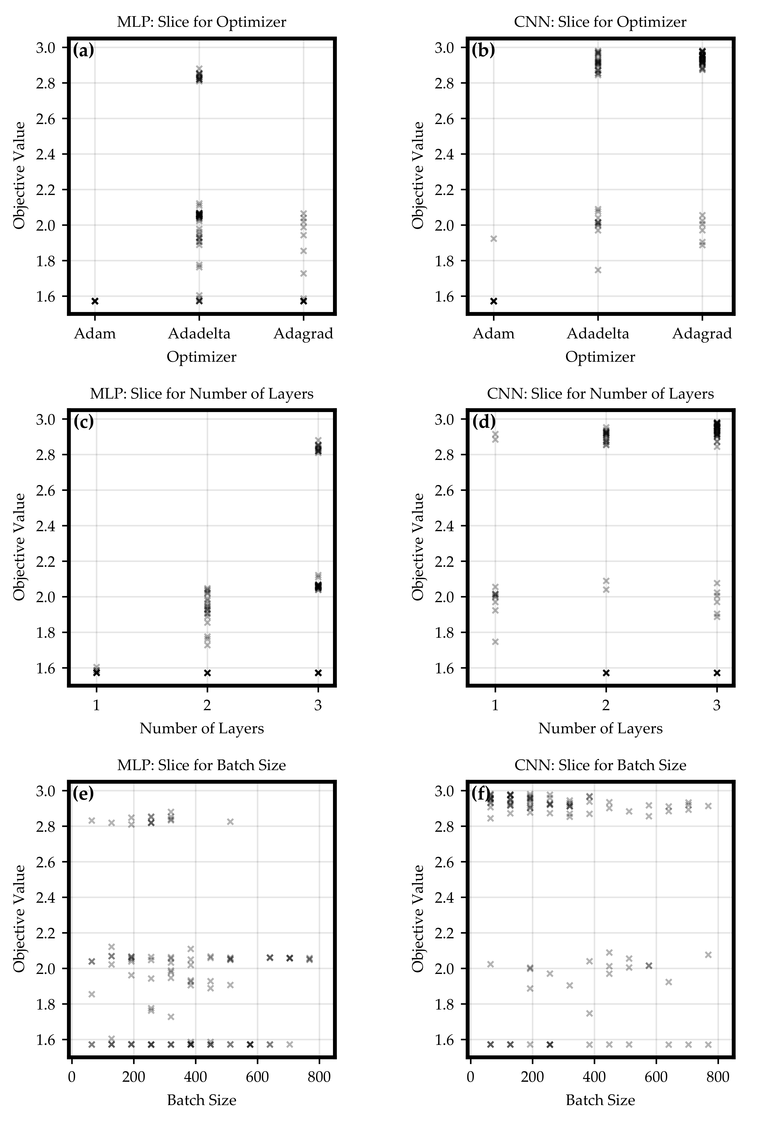
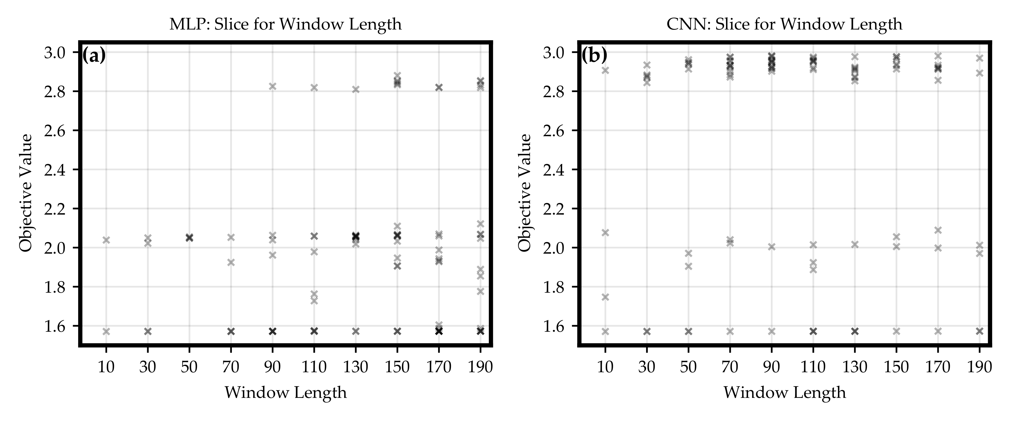
In Section 3.1, hyper-parameter optimizations for MLP and CNN classifiers were executed. The results led to the conclusion that both architectures can be configured such that a trained network is able to solve the classification task formulated in this paper. Nevertheless, the CNN optimization obtained a higher number of classifiers which were able to achieve satisfying objective values. For most of the regions of the hyper-parameter space, there were choices returning objective values close to the maximum of 3. For example, even CNN models with only one convolutional layers were able to get a relatively high objective value. Because of theses reasons, it can be suspected that for a classification task with more trainable loads and more active participants in the grid the CNN architecture would rather lead to an accurate recognition and a clear separation of the trained classes than an MLP.

After hyper-parameter optimizations, a best MLP and a best CNN was determined. Even if the CNN classification in the validation scenarios yielded the overall best objective value, this value dropped significantly at node $N1$ of the MONA reference grid.

The recognition ability of these best neural networks was investigated more precisely to examine the mentioned accuracy drop.

In Section 3.2.1, load and inverter were assumed at the same grid node and the line distance between this node and the transformer was varied. This test case proved that larger distances between the transformer and the measurement point or inverter, respectively, improves the recognition. Furthermore, the CNN was able to achieve the threshold of 90% at less distance than the MLP, and it can be concluded that inactive classes are more accurately classified by the CNN.

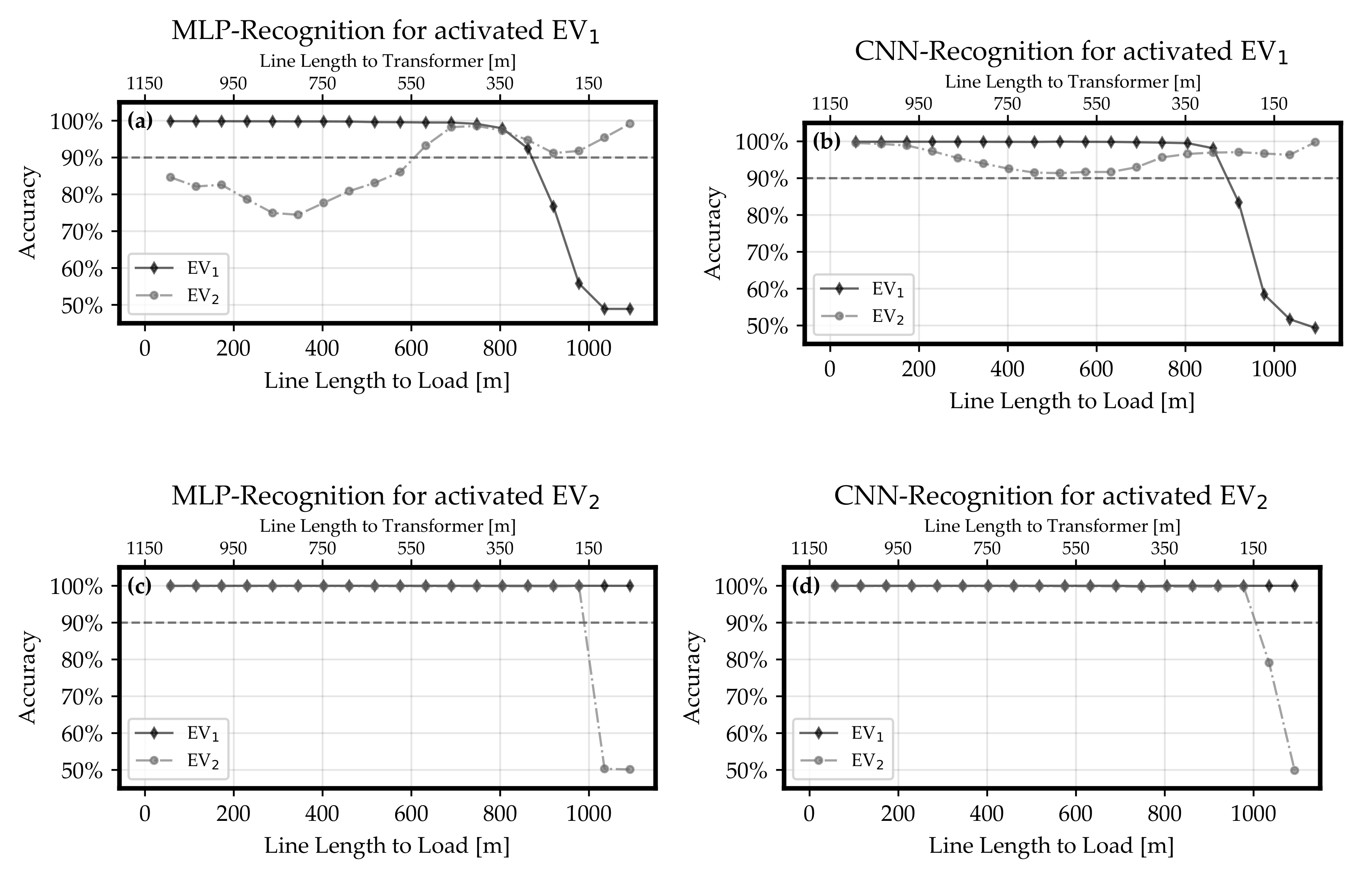
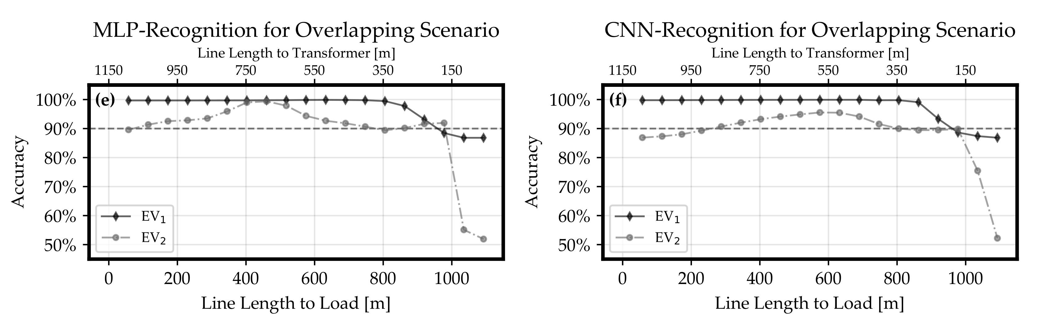
Section 3.2.2 answered the question what happens if load and inverter are not located at the same grid node. It could be shown that an increasing line length between inverter and load decreases the accuracy of recognition. Regarding this relation, the CNN was able to remain the accuracy for active loads above the 90%-threshold with higher line length between inverter and load than the MLP. Similarly to Section 3.2.1, the recognition results for the CNN classifier were more accurate regarding inactive classes. In this study, an increasing line length between inverter and load meant a larger area inside the power grid which was observed. Therefore, the CNN can be seen as the preferable classifier because more information from the grid can be gathered in a reliable manner.

From both parts of Section 3.2, it can be concluded that classifiers trained by the proposed concept are able to provide a reliable load recognition inside typical power grid structures if they are located around hundreds of meters away from the transformer and also the distance between measurement point and active load is in the range of hundreds of meters. Thereby, the more accurate performance of the classifier in scenarios with activated EV${}_2$ compared to cases when EV${}_1$ is active indicates that less fluctuating profiles can be recognized with higher accuracy. The highly accurate results in the test cases of this study are very promising. Especially the CNN’s potential did not have to be fully exploited in the test conditions as there were many configurations with high objective values.

In this framework, the recognition is based only on the voltage changes caused by active loads. On the one hand, this approach does not need an extensive amount of data. In further development of this concept, it is an interesting research question to integrate more different load types into this recognition task. Here, one line of investigation could be the approach of incremental learning [53,54,55]. New classes can be included in the training data without a huge simulation effort. If one characteristic profile for a new class is available, it can be trained and the corresponding recognition results can be analyzed afterwards.

On the other hand, this approach is limited because it depends on the magnitude of the voltage changes. If these changes at the point of voltage measurement are very small, it is not possible to recognize a particular profile. In this case, it is possible to train the neural network classifier inside the proposed simulation environment with differently scaled training data such that it is more sensitive to smaller changes. This adaption would not be appropriate in real world application because of the background noise in the power grid and other external effects to consider. Additionally, in the use case of voltage control it is intended to recognize not every single small or distant load but the loads with large impact to the grid voltage to determine an optimal control strategy for grid-stabilization. The particular voltage behavior at a single grid connection point is affected by the overall grid topology, the size of active loads and their position in the grid, and also the activity of other loads. This means, the limitation depends on many factors for the load recognition and is still under research.

Despite the limitations not yet explored, the quite simple demonstration example of two EVs presented in this paper is sufficient to conclude that the proof of the proposed concept was successful. The detailed potential in real world applications will be part of future work. For example, to enable the classification algorithm for load recognition under consideration of uncertain and fluctuating feed-in of renewable energies, the particular training dataset should be extended. This means, the neural network could be trained by voltage profiles which are modified by statistical noise in addition to scaled and overlapped profiles. Additionally, due to the increasing complexity it might be necessary to add more layers to the neural network.

5. Conclusions

In this study, a new concept to recognize active load classes in the local grid environment of an inverter’s grid connection point based on the locally measured voltage was presented. The proposed concept formulates the recognition task as a multi-label classification of time series windows and uses neural networks as a classifier. For demonstration and a proof of concept, the methodology was applied in an example of two electric vehicles in a simulated test environment. This approach was tested in Section 3 regarding the influence of the inverter’s distance to the transformer and the particular active loads. It turned out that a classifier trained by the proposed concept is able to recognize different load types in the voltage signal. A usage of CNNs for recognition instead of MLPs yields higher accuracies in general. Hereby, the recognition accuracy is increased by an increasing distance between transformer and measurement point, and decreased by an increasing distance between load and measurement point.

In summary, a concept for a load recognition in low voltage distribution grids based on deep learning was developed and validated in a simulation environment. Future work can investigate the concept with an increased number of active loads in the grid and more trainable classes. Additionally, the recognition approach will be transferred into a real hardware environment. By this, the measurement will include background noise and measurement errors, for example, such that the input data for the algorithm is partially disturbed. This will challenge the algorithm to be robust to those disturbances and to decide whether a slightly changed voltage pattern still belongs to a trained class, or not.

In future, this concept can be used to gain knowledge about the local grid environment of an inverter’s grid connection point. Therefore, it can be implemented in a voltage control algorithm to set active and reactive power adapted to the grid node specific conditions. Consequently, it can contribute to a future stabilization of the grid voltage in a significant manner.