Article

A Proportional Digital Controller to Monitor Load Variation in Wind Turbine Systems

by
José Gibergans-Báguena
1,†,
Pablo Buenestado
2,†,
Gisela Pujol-Vázquez
1,*,† and
Leonardo Acho
1,†
1
Department of Mathematics, ESEIAAT-Universitat Politècnica de Catalunya (UPC), 08222 Terrassa, Spain
2
Department of Mathematics, EEBE-Universitat Politècnica de Catalunya (UPC), 08019 Barcelona, Spain
*
Author to whom correspondence should be addressed.
These authors contributed equally to this work.
Energies 2022, 15(2), 568; https://doi.org/10.3390/en15020568
Submission received: 21 December 2021 / Revised: 10 January 2022 / Accepted: 11 January 2022 / Published: 13 January 2022
(This article belongs to the Special Issue Wind Turbine Structural Control and Health Monitoring)

Abstract

:
Monitoring the variation of the loading blades is fundamental due to its importance in the behavior of the wind turbine system. Blade performance can be affected by different loads that alter energy conversion efficiency and cause potential safety hazards. An example of this is icing on the blades. Therefore, the main objective of this work is to propose a proportional digital controller capable of detecting load variations in wind turbine blades together with a fault detection method. An experimental platform is then built to experimentally validate the main contribution of the article. This platform employs an automotive throttle device as a blade system emulator of a wind turbine pitch system. In addition, a statistical fault detection algorithm is established based on the point change methodology. Experimental data support our approach.

1. Introduction

Wind turbines are a rapidly growing renewable energy option in today’s world [1]. However, these machines require maintenance approaches, for instance, to prevent malfunctions during power production [1]. Therefore, monitoring the variation of the loading blades in wind turbines is an important issue. This is because the dynamic of the blade system is affected by different loads that alter the efficiency of energy conversion and also, the possibility of causing potential safety hazards [2,3]. The deterioration or damage of wind turbine blades not only causes problems in the efficiency of power generation, but also induces vibrations, increasing safety risks and maintenance costs. A full review on this topic can be found at [4]. An example of deterioration or damage to wind turbines is the formation of ice on their blades [5]. A blade system is an electromagnetic device located at the rotor of a wind turbine able to rotate longitudinally in both directions [1]. Figure 1 illustrates the main structure of a wind turbine. In the literature, there are many contributions to detect faults in the pitch actuators of wind turbines [6]. In [7], the authors provide a machine learning algorithm for the data imbalance problem in detecting icing faults in wind turbine blades, also presenting numerical simulations. Obviously, the machine learning method is a methodology in the state of the art of artificial intelligence. However, we seek to employ more standard techniques. Moreover, in [8], a pitch actuator monitoring system is proposed by using interval observers. In [9], a pitch actuator fault detection method is presented by using a digital disturbance observer. Image processing is also used to monitor the performance of a pitch actuator system [10], including the use of laser and acoustic technologies [11]. All of these reports focus solely on the pitch actuator system, but the case of directly monitoring load variation on the pitch system seems like a new approach.
In the past, in robotic applications, a closed-loop system with the conventional proportional controller in it was shown to exhibit a constant error that is dependent on external forces [12]. Therefore, this controller is also sensitive to load variation. This simple fact is used here to propose a methodology to detect load variation on wind turbine blades. This is the main objective of this work. On the other hand, micro-controllers or embedded systems have been used for many years in modern electronic devices. For instance, the PIC18F252 micro-controller provides good performance as a digital signal processor. This micro-controller is used here to program a digital proportional controller to the throttle device as an emulator of a pitch-blade system. An automotive throttle device can emulate a wind turbine blade system, capturing some severe non-linearities, such as backlash, friction, and load variations, among others [13]. About the precision of the emulation of the real object by the proposed emulation platform, and according to [14], the precise prediction of the load variation dynamics of wind turbines with experiments is complex due to many non-linear factors of the wind turbine pitch system mechanism. However, experimentation is used for the validation of dynamic models used for the analysis of real wind turbines [14]. See Figure 2 and Figure 3 for a diagram overview of the emulator. Both devices control a rotation system: the wind turbine pitch actuator keeps the rotor blades at the required angle, while the throttle system drives its angular position of the throttle plate to the desired reference position. Moreover, both are affected by complex non-linearities [13]. By similarity with the automotive throttle device, the returning springs may capture the load produced by the wind turbine on the blade (see Figure 2). In particular, modifying the throttle’s electronic system, a load variation in wind turbine can be modeled and seen as ice on the blade. It is well known that the accumulation of ice on the surface of the blades changes its shape and mass, causing an imbalance on the rotor that is rotated mainly by the lift force that comes from the wind [15]. The same effect is produced when an external resistance is added to the electronic circuit of the throttle valve. Hence, and from the experimental point of view, a digital controller is realized to manipulate a throttle device, where a load variation of the throttle plate is also experimentally implemented. Therefore, this experimental platform will emulate a pitch actuator system with load variation on the blade. According to the experimental data, the digital proportional control with our processing method can monitor the load variation in the cited system. To design a low cost experimental wind turbine emulator, the simplicity of the controller is a must.
Therefore, once the experimental data are obtained, a fault detection algorithm is designed, based on the change point detection (CPD) methodology. [16]. The problem of detecting points of change in the data has its origin in the quality control methodology, where the main objective is to monitor the performance of an industrial manufacturing process by detecting failures in it [17]. However, this problem is very general in nature, and change detection techniques have been further applied to various branches of research: climatology analysis [18,19], medical analysis [20], remote sensing [21], image analysis [22], business [23], and so on. In addition, many types of algorithms have been developed to solve this type of problem statement [24,25]. In our work, some of these techniques are used in order to detect when a failure of the aforementioned system has occurred.
The main contributions of this work can be summarized as follows:
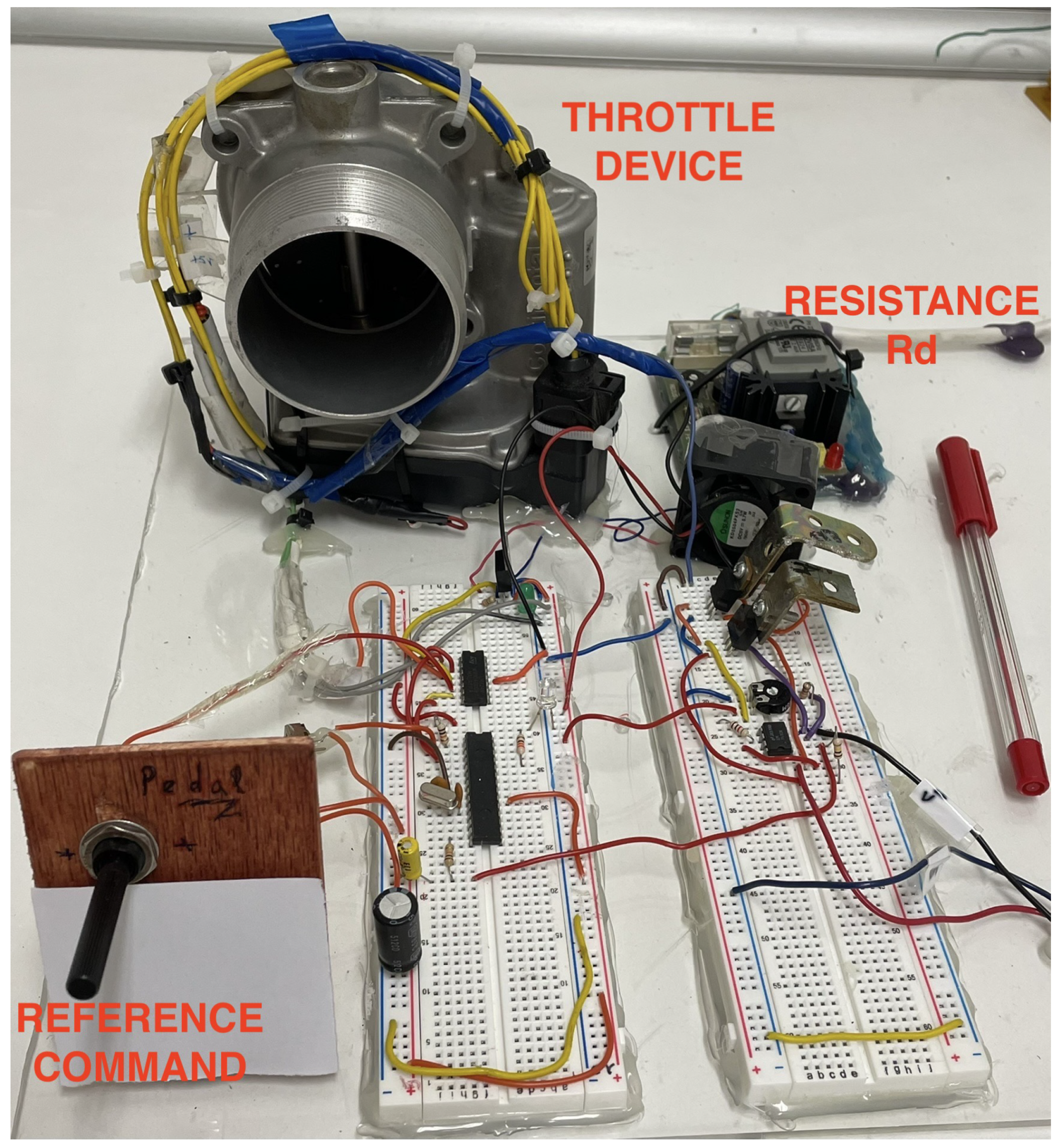
  • Design of an experimental platform capable of reproducing the load variation in a wind turbine blade system. The electronics accompanying the throttle valve are modified to emulate the use of a real wind turbine with varying load on the blades.
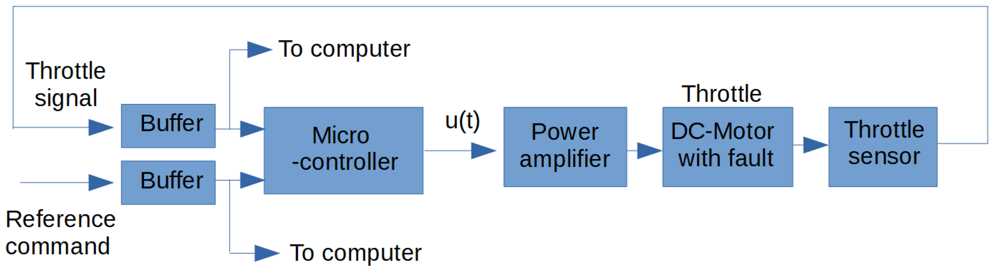
  • Implementation of a proportional digital micro-controller capable of detecting load variations.
  • Define an algorithm that allows the detection of failures by studying only a specific statistical parameter, such as the statistical point change detection method.
The novelty of this paper is then the direct monitoring of the load variation, designing a novel experimental platform and obtaining from it an statistical rule of decision to detect a failure system.
This paper is organized as follows. Section 1 describes the problem formulation. Section 2 presents the experimental part of this work, followed by its results on a faulty scenario. The study of the experimental data, as well as the definition of a detection algorithm is presented in Section 3. Some experimental tests of the fault detection method are discussed in Section 4. Finally, Section 5 states the conclusions.

2. Materials and Methods

This section presents the backgrounds of the experimental realization of a proportional controller to the selected throttle device. Figure 4 displays a photo of the developed experimental platform. This platform is composed of the throttle device, where the blade system is reproduced; a resistor that performs the load variations; a trimmer for manually inputting the reference signal; and the electronic circuit that connects all these devices with the microcontroller, where a digital proportional control is programmed.

2.1. Load Blade Emulator

This subsection shows how to emulate a load variation using a resistor on the throttle device electronics. That is, we present the mathematical model of load variation in the throttle device to emulate the load variation on the blade body of a wind turbine. As stated in the Introduction section, the automotive throttle device may emulate a pitch system of a wind turbine. Due to the throttle system having a (permanent) DC motor to manipulate the throttle plate, it can be used to simulate a load variation. Let us consider a representative model of a DC as shown in Figure 5 [26]. Here, u ( t ) is the control input (V); i a , R a , L a , and K b are the armature current (A), the motor internal resistance ( Ω ), the motor armature inductance (H), and the back electromotive force constant (Vs/rad), respectively. w ( t ) , J, and b are the motor speed (rad/s), the motor load (Kgm2), and the coefficient of viscous friction (Nms/rad), respectively. In this scheme, we add a motor load variation emulator via the resistance R d ( Ω ). To add, there are two assumptions implicit in our approach:
Assumption 1.
Because we are working on a closed loop system capable of generating data for fault diagnosis, the closed-loop system is required to be stable in the sense of the bounded-input bounded-output definition rather than in the asymptotically stability statement.
Assumption 2.
The operation of the wind turbine is within the operating range.
Therefore, the mathematical of the electromagnetically permanent DC motor is [26]
L a d i a ( t ) d t = u ( t ) ( R a + R d ) i a ( t ) k b w ( t ) ,
J d w ( t ) d t = k t i a ( t ) b w ( t ) ,
where k t is the torque constant (Nm/A).
Usually, the electric transition dynamic in (1) is faster than in (2). Because of it, we can obtain the equilibrium point in (1) and then replace it into (2), yielding
J ( R a + R d ) d w ( t ) d t = k t [ u ( t ) k b w ( t ) ] b w ( t ) [ R a + R d ] .
From the above equation, we can see that the resistance R d emulates a load variation on the motor load. In fact, this strategy to use a resistance in series to a DC motor to emulate a dummy motor load was previously invoked, for instance, in [27]. Hence, given the system operating at nominal load, J f = J R a , and the loaded case J I = J ( R a + R d ) , we have
J f J I = J ( R a + R d ) J R a = 1 + R d R a ,
Therefore, R d R a is the percentage of load added to the nominal scenario. Finally, consider the control law given as a proportional one:
u ( t ) = K p ( β ( t ) β r e f ) .
The simplicity of the controller in (5) allows to introduce a load variation in terms of an external resistance R d , as the closed loop demonstrates. That is, using w ( t ) = d β ( t ) d t , the closed-loop system (3)–(5) yields
d 2 β ( t ) d t 2 + k t k b + b ( R a + R d ) J ( R a + R b ) d β ( t ) d t + K p k t J ( R a + R d ) β ( t ) = K p k t J ( R a + R d ) β r e f
From the above equation, it is clear that the transient response and the steady-state solution of this closed-loop system will depend on the loading scenario. That is, resistance R d affects the closed-loop system (6) as a load variation modifies the wind turbine dynamics. Moreover, our fault monitoring algorithm will detect these variations for diagnosis, as presented in Section 4.

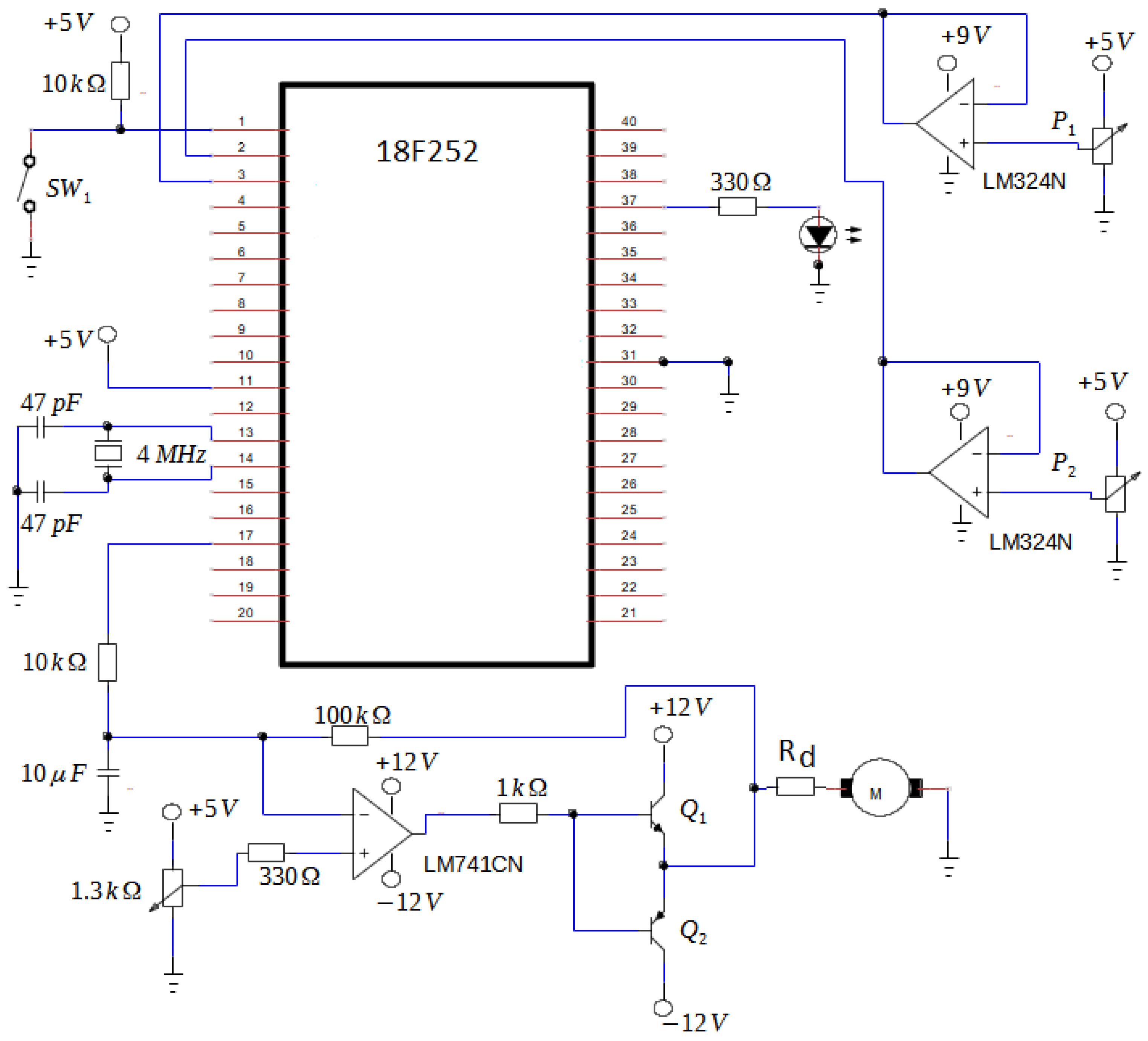
2.2. Electronic Circuit Design

See Figure 6 for a detailed scheme of the electronic circuit design in conjunction with the digital controller programmed into the PIC 18F252 micro-controller to manipulate our throttle device. Moreover, Figure 7 shows the design process of this electronic realization.

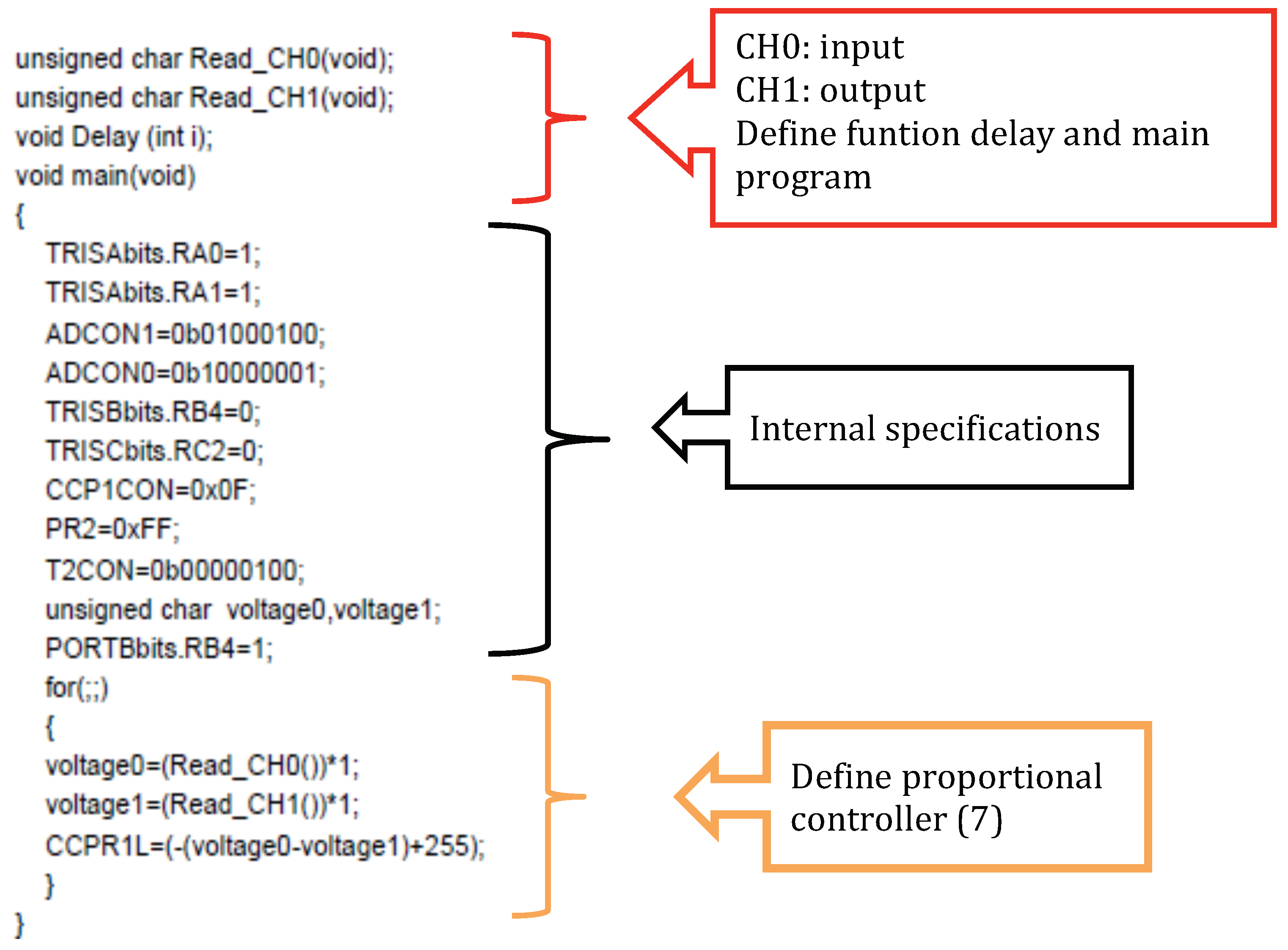
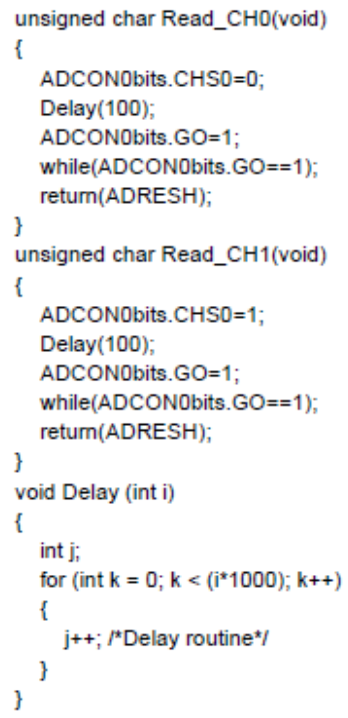
2.3. Micro-Controller Programming

The micro-controller in Figure 7 was programmed in C language. The micro-controller read two signals: (1) the signal supplied by the throttle-plate angular position sensor, and (2) the other from the reference command information (both in the interval from 0 to 5 volts). The throttle sensor is linear where a reading of about 0.79 volts corresponds to the closed-plate position of the throttle device, and a reading of about 4.6 volts when this throttle plate is fully open, as shown in Figure 8. Therefore, the reference command should be in the same interval of voltage. The throttle sensor is implemented by using a potentiometer (trimmer). This is done by the manufacturer. We also use a potentiometer to supply the reference command manually. The electronics interface of these potentiometers data to the micro-controller is via operational amplifiers. We use the buffer configuration (see Figure 6). Therefore, the micro-controller is programmed to read these data approximately every 5 ms of a time interval. On the other hand, it is well known that most modern micro-controller units have built-in pulse width modulation blocks as a low-cost approach to convert digital data to an analog signal by using an external RC circuit (see pin number 17 of the micro-controller unit in Figure 6). Therefore, our micro-controller unit was also set to produce a pulse width modulation signal related to the proportional controller command:
C C P R 1 L = ( ( v o l t a g e 0 v o l t a g e 1 ) + 255 ) ,
where C C P R 1 L is the produced control signal u ( t ) in the pulse width modulation format, and v o l t a g e 0 and v o l t a g e 1 are the signals from the throttle sensor and the reference command, respectively. The 255 added value in (7) is because the reading inside the micro-controller unit goes from 0 to 255 when an analog input signal goes from 0 volts to 5 volts, respectively. This offset value is then subtracted by the potentiometer (trimmer) of 1.3 kilo-ohms shown in Figure 6. Finally, this control law is amplified by an factor of about 10 units by the operational amplifier L M 741 C N given in Figure 6. Hence, the analog version of the controller signal seen by the motor corresponds to (5) with proportional parameter K p set at 10:
u ( t ) = 10 ( β ( t ) β r e f ) .
Finally, the C-program stated in Appendix A details the configuration settings of the micro-controller unit along with the proportional controller law. This program is self-explanatory due to the C programming language and knowledge of micro-controller architecture.
We use a proportional controller not only for its simplicity, but more importantly because it allows us to see how the external resistance in the acceleration system emulates a load variation in the wind turbine system, as indicated in Section 2.1.

3. Results

In this section, the experiments are carried out, and then the fault detection algorithm based on the change of point detection methodology is established, taking into account Assumptions 1 and 2 established above in the Introduction section.

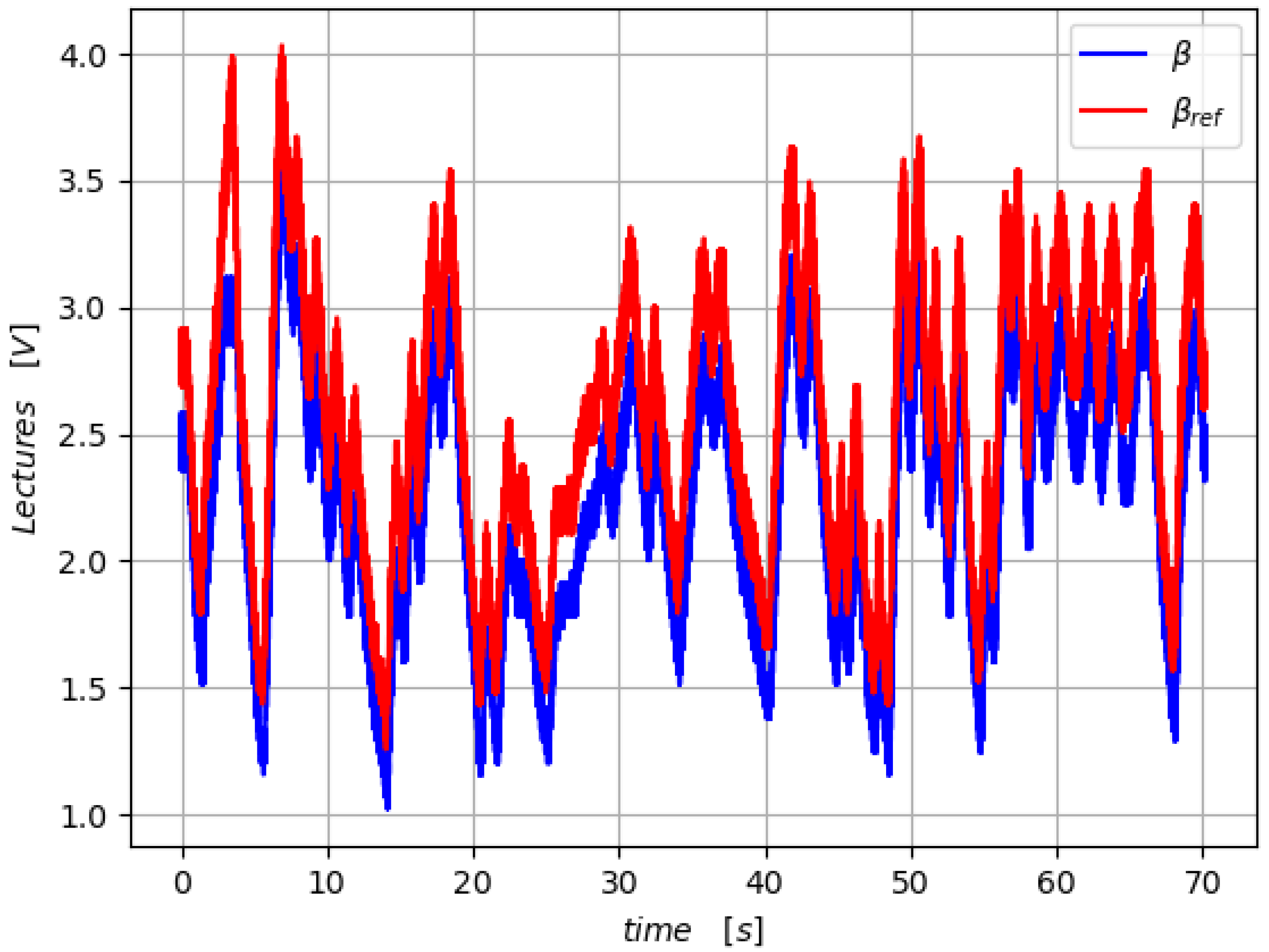
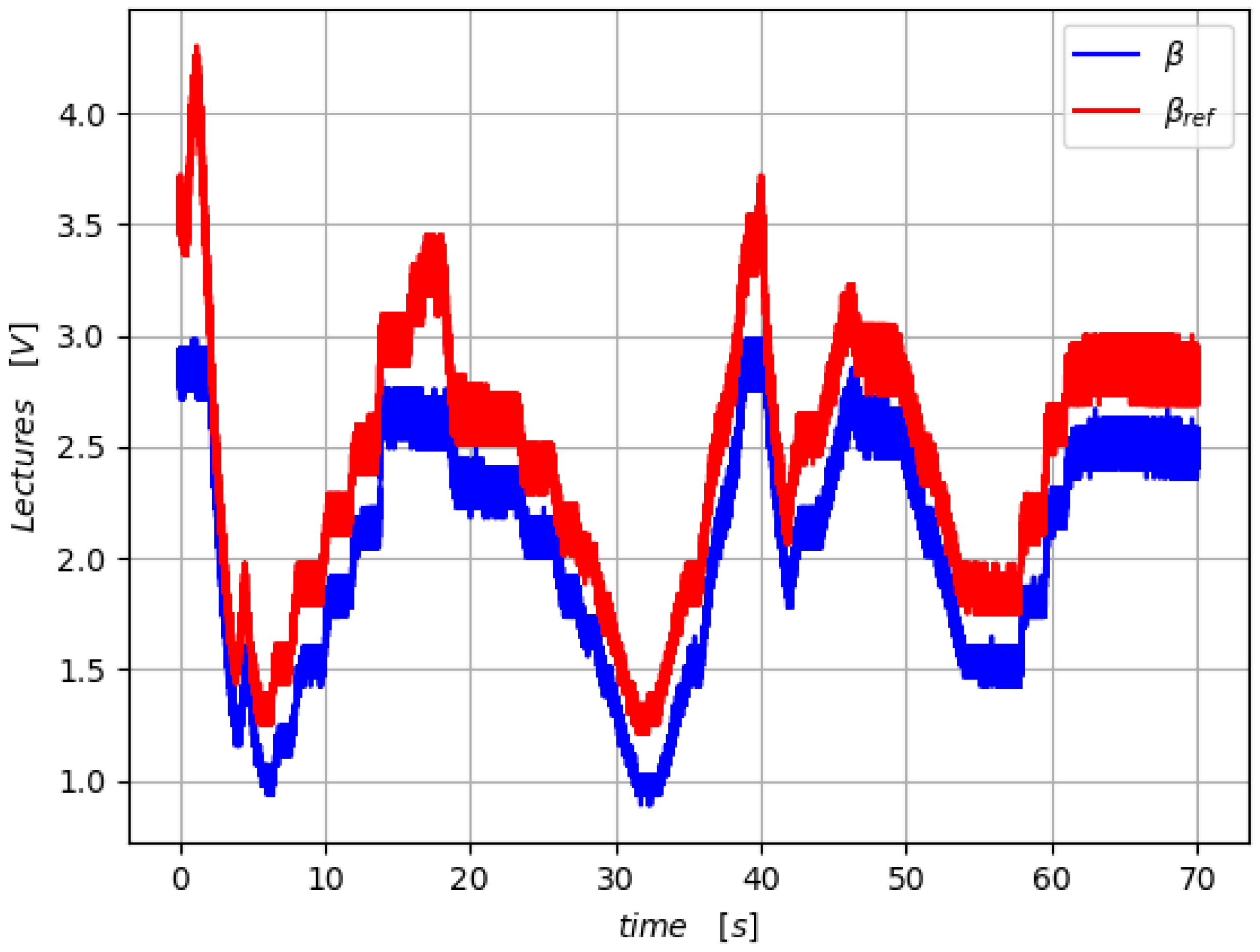
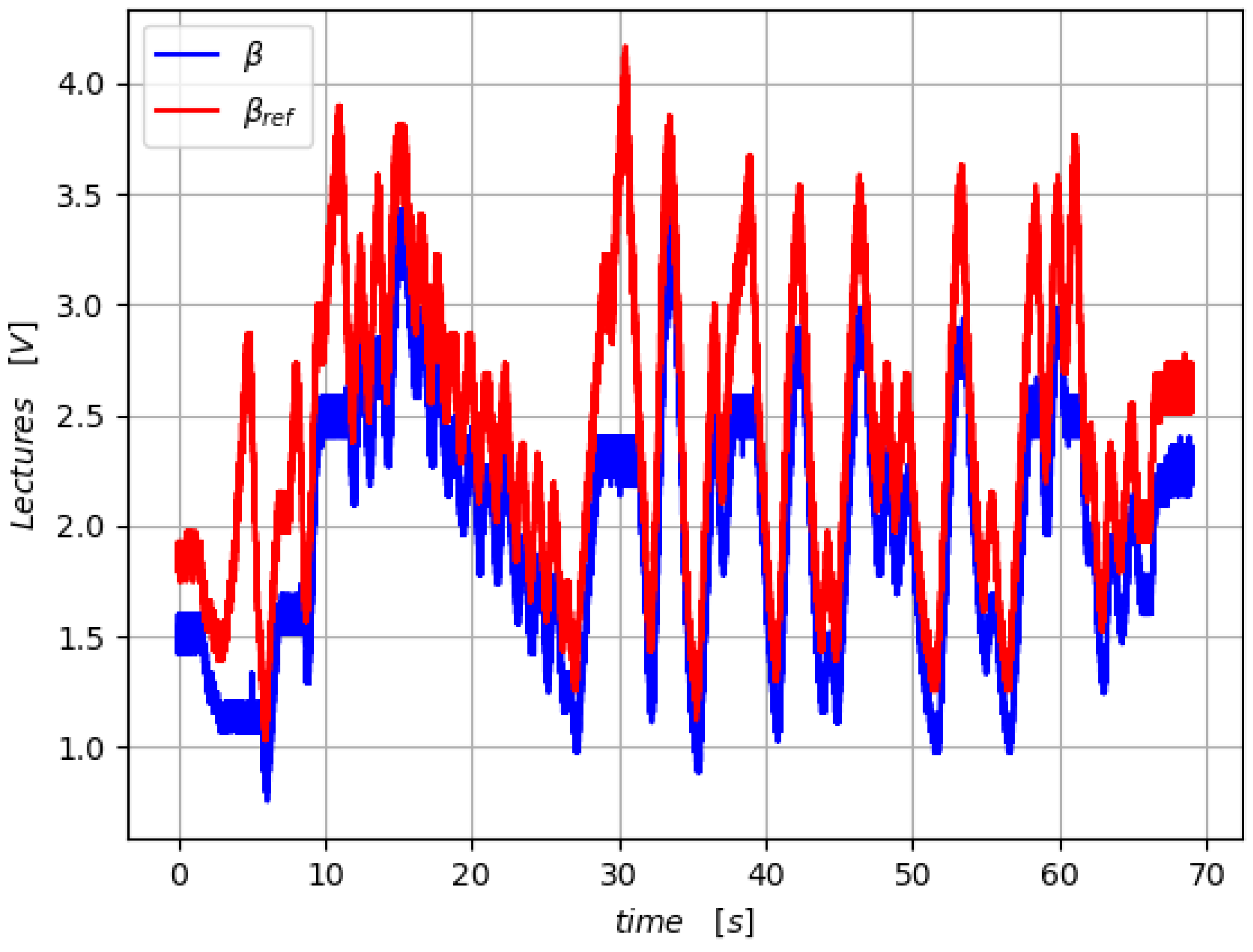
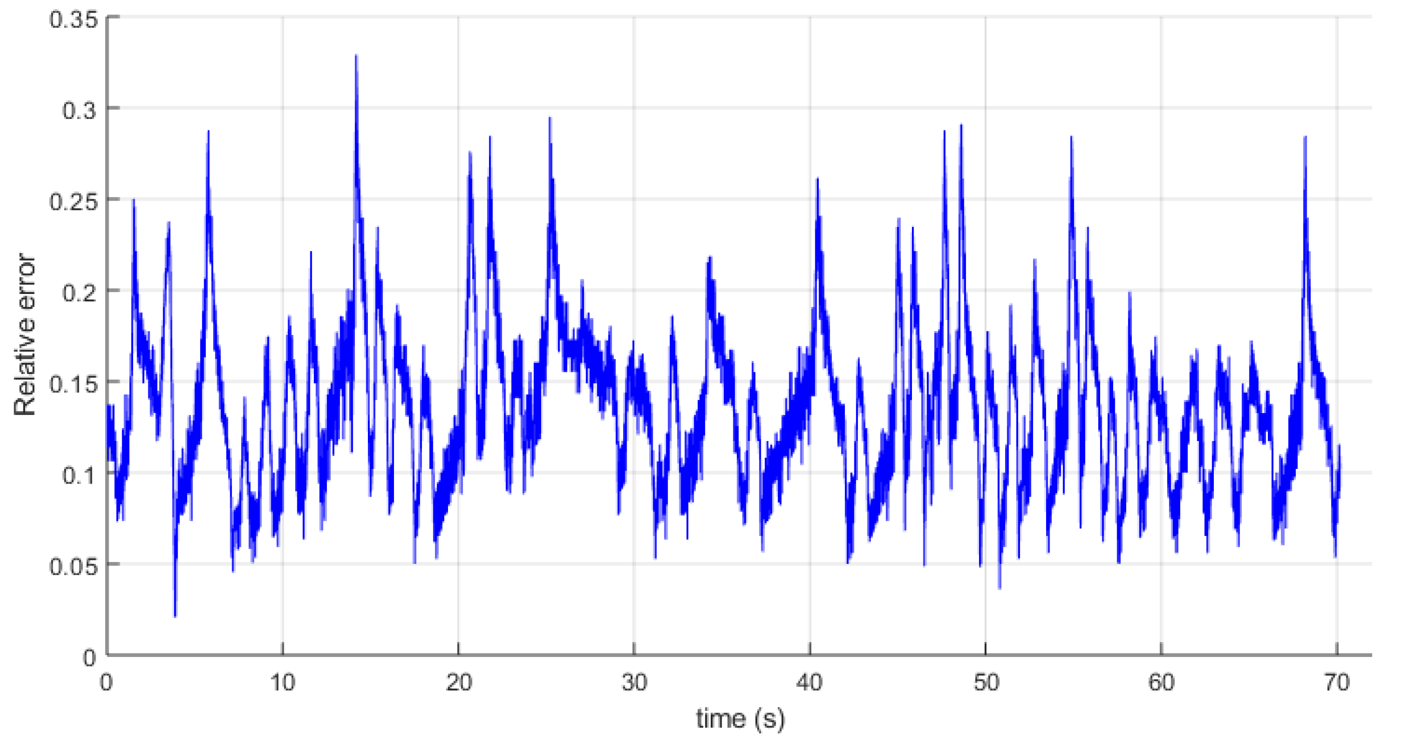
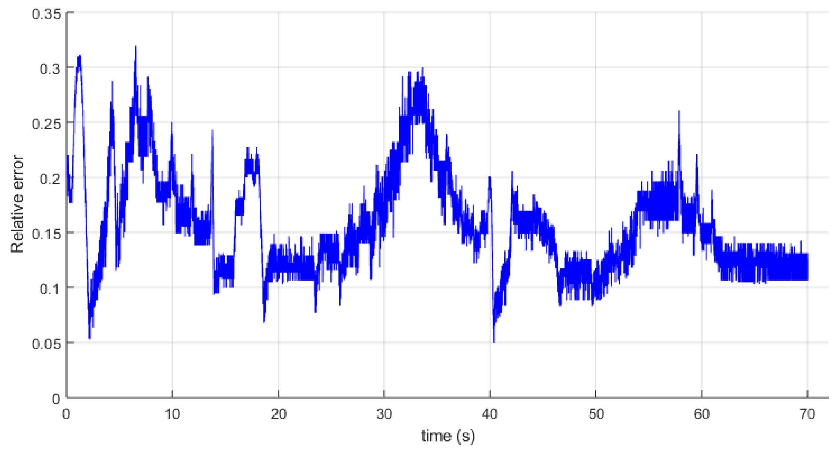
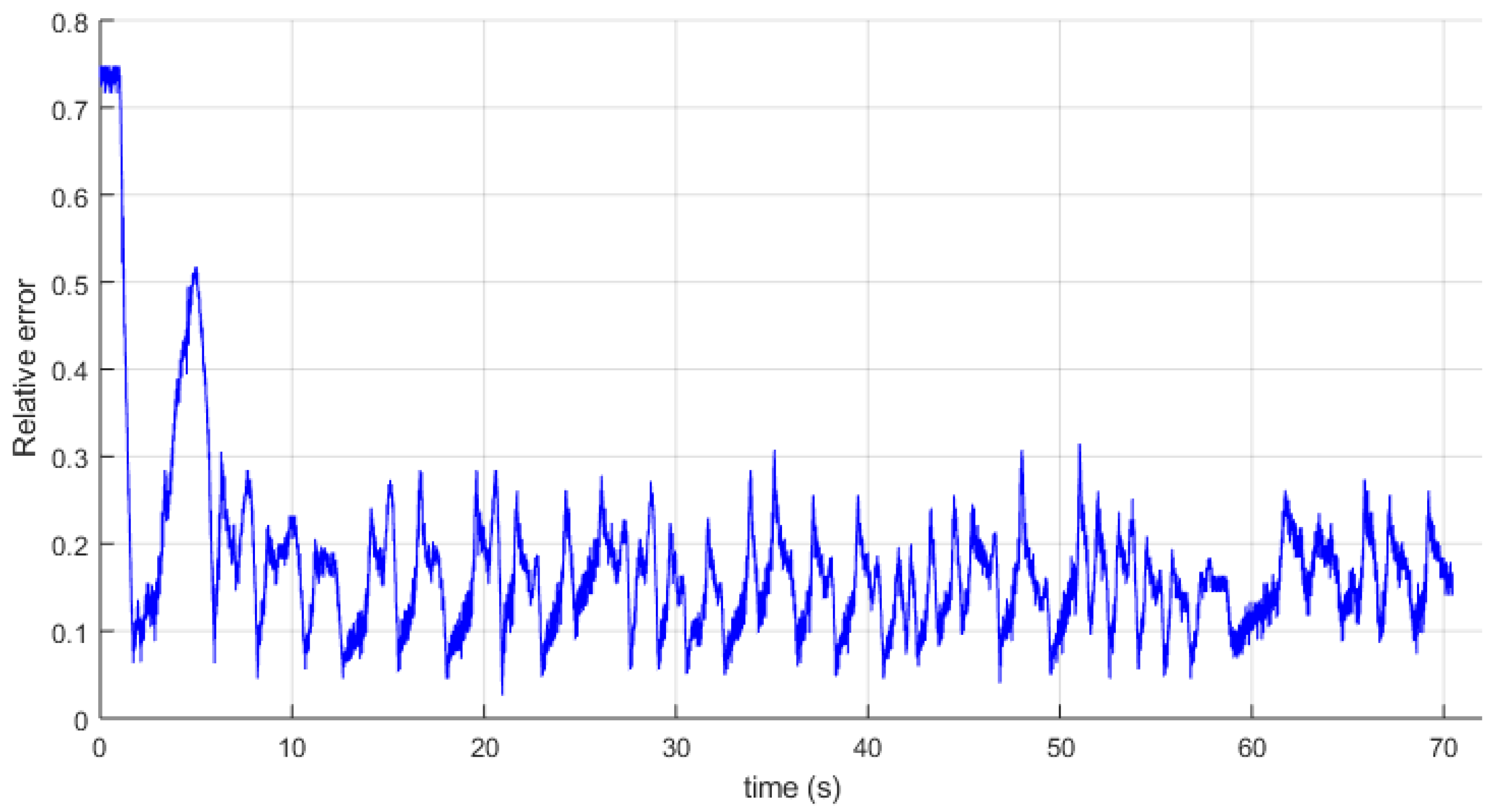
3.1. Experimental Data

The micro-controller reads the data from the throttle sensor and the reference command. These readings are accomplished by the micro-controller’s data acquisition system. Figure 9 and Figure 10 show two experimental results with R d = 0 ohms. These simulate a normal pitch system operation (the no loading case). For future reference, we label them as N 1 and N 2 , respectively. On the other hand, Figure 11, Figure 12 and Figure 13 show three experiment outcomes but now with R d = 0.5 ohms. These three ones represent the failure situations (the loading case). We name them F 1 , F 2 and F 3 for faulty cases. Therefore, we have five experiments realized randomly.
It is important to note that fault detection in our system becomes difficult if we directly analyze these experimental data. Therefore, a more detailed study should be carried out.

3.2. Experimental Correlation with a Real Wind Turbine

The main objective of this section is to experimentally validate our experimental platform in comparison to a real wind turbine related to its pitch system. It is well known that a wind turbine pitch system can be modeled by a linear and time-invariant second-order system [8,9,10]. Therefore, the response time of a hydraulic pitch system for a wind turbine is set as τ s = ζ w n 6.666 s [8,9,10]. Thus, the settling time can be inferred as five times this value, which is approximately 33.33 s. Let us estimate our settling time in our emulator system by using the experimental data previously described and displayed in Figure 9. Let us begin by using a first-order linear system of a pith system [28]:
β ˙ ( t ) + a β ( t ) = a β r e f ,
where a is the system parameter related to its time constant value. Based on, and motivated by, the previous equation, we propose the following parameter observer:
a ^ ( t ) = β ^ ˙ ( t ) p r o j ( β r e f β ( t ) ) ,
where
p r o j ( · ) = · if · > θ * s i g n ( · ) θ * if · θ * ,
and β ^ ˙ ( t ) is an estimation to β ˙ ( t ) obtained by using
G ( s ) = s τ s + 1 = y o ( s ) β ( s ) .
Then, y 0 ( t ) = β ^ ˙ ( t ) . Finally, the next dynamic is used for the settling-time observer to our system:
z ˙ ( t ) = α [ a ^ ( t ) z ( t ) ] if a ^ ( t ) z ( t ) > 0 γ z ( t ) if a ^ ( t ) z ( t ) 0
The above dynamic is considered a peak detector system [29] but by adding a forgetting factor. By using the data in Figure 9, Figure 14 shows the obtained result of the proposed observer giving z ( t ) . Here, we can observe that the settling time observer is changing in response to several non-linear effects of the emulated pitch-blade system as expected from the real blade dynamic on the pith actuator on load variation, for instance, due to the wind on the blade. Additionally, the average of the value is commensurable to the previous one of 33.33 s.

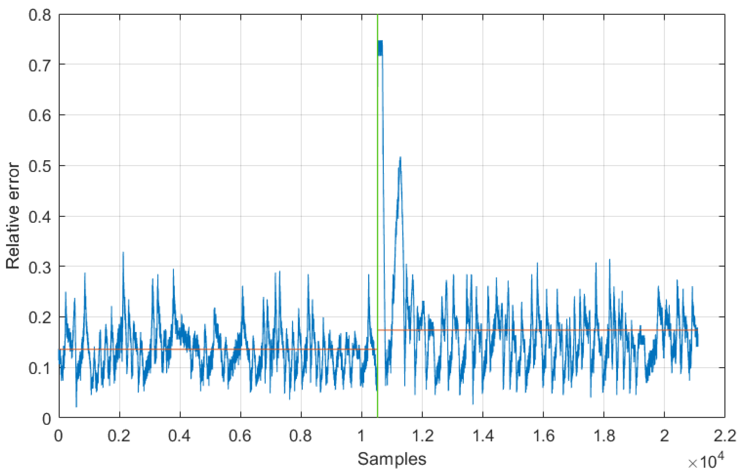
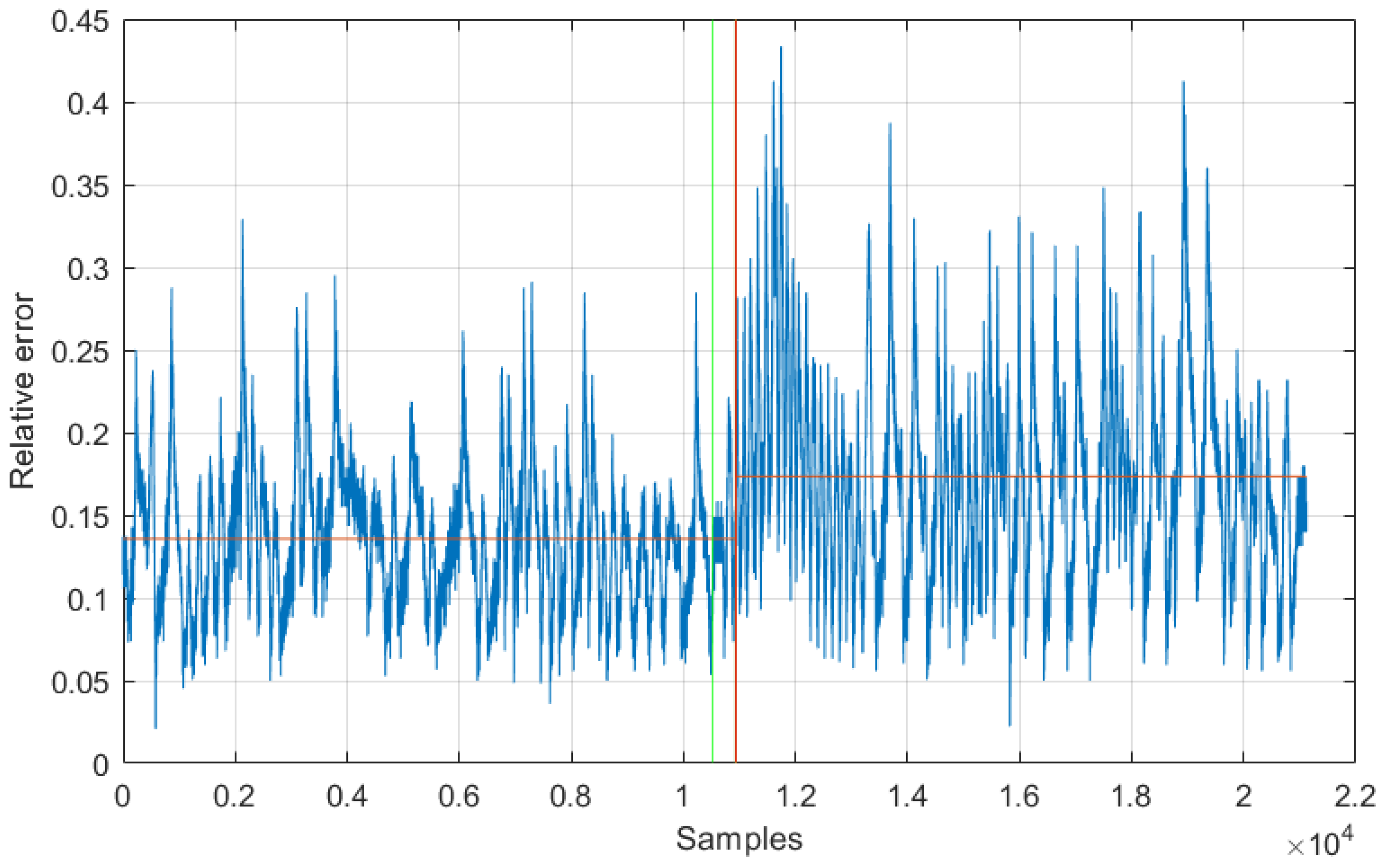
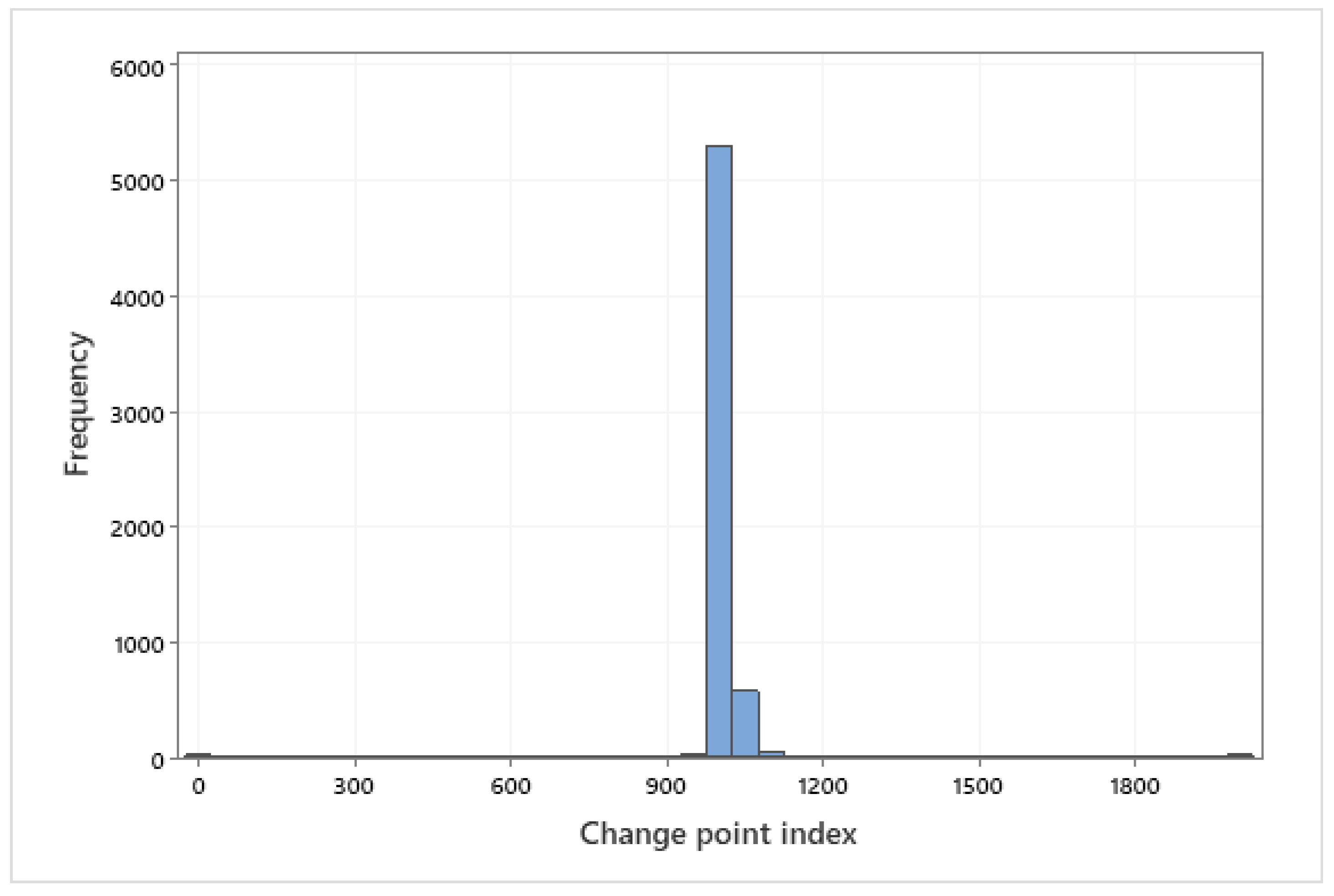
3.3. Statistical Diagnosis of Fault Detection

The obtained experimental data are analyzed to establish a discrimination criterion between the normal and the faulty scenarios. As mentioned in the introduction, our approach uses the change point detection (CPD) methodology [16], where the main objective is to monitor the performance of the blade system by detecting failures (load blade variation) in it [17]. That is, to discuss the performance of the digital proportional controller (7) to produce useful data to monitor load variation. We first present the statistical approach used in this document. Once the detection algorithm is described, a detailed discussion is presented.
To have data series independent of the reference measures, first, the relative error is calculated for each series, that is,
ε = β β r e f β r e f .
Therefore, for each case under study, we obtain the relative error ε c (14), where c is named for each experiment. Thus, we have the following data series: ε N 1 , ε N 2 , ε F 1 , ε F 2 and ε F 3 , whose graphic representations are shown in Figure 15, Figure 16, Figure 17, Figure 18 and Figure 19. Then, when comparing them, it is difficult to appreciate a load variation in the emulator experiment.
So, a first statistical analysis of the previous series is carried out and presented in Table 1 and Figure 20 and Figure 21, where dot plots and boxplots of tracking relative errors are pictured. Table 1 presents, for each experiment, its dimension N, arithmetic mean (mean), standard deviation (std), minimum value (min), maximum value (max), and the three quartiles ( Q 1 , Q 2 , and Q 3 ) [30]. Therefore, the experimental data series are classified into five groups of equal size.
From Figure 20, it is observed that all the experimental data present positive asymmetry, but higher for the faulty cases. From Table 1 and Figure 21, it can also be seen that the arithmetic means, standard deviations, and Q 2 and Q 3 quartiles are always higher in failure cases. Therefore, there is a large statistical difference between the nominal and failed operating cases. Consequently, it should be possible to discriminate when the system goes into failure using the change point detection (CPD) methodology, as expected [16]. In this work, we avoid using indices on the quality of fault detection, such as accuracy, sensitivity, precision, area under the ROC curve (AUC), etc., by using the change point detection (CPD) method. However, a detailed study of the accuracy of our method is presented in Appendix A. This method uses the minimization of the residual information of the error, which is equivalent to maximizing the logarithmic likelihood. So, this method has a sensitivity value greater than 0.75 [31], which is good performance for our intention.
Let us consider the case where a change occurs during data capture. That is, there is a change in the same data series when the system goes from a normal case to a faulty one, for example. To begin with, given a series x 1 , x 2 , , x N , the CPD technique divides the series into two regions, x 1 , x 2 , , x k 1 and x k , x k + 1 , , x N so that the sum of the residual error (square) of each region is minimized from its local statistical parameter (arithmetic mean, standard deviation, etc.) [16]. Hence, we must find the value of k that minimizes the CPD index [16]:
J ( k ) = i = 1 k 1 Δ ( x i ; χ ( [ x 1 , , x k 1 ] ) ) + i = k N Δ ( x i ; χ ( [ x k , , x N ] ) ) ,
where you are given the empirical estimate of the section of the local statistical parameter χ and the measure of the deviation Δ with respect to the chosen statistical parameter [16].
Previously, it was observed that, in our experiments, the arithmetic mean and the standard deviation are good statistical values capable of differentiating between normal and faulty stages. In these cases, we have the following:
  • If the mean is used to detect changes in the series, then the CPD index (15) is defined as (where v a r denotes the variance):
    i = m n Δ ( x i ; χ ( [ x m , , x n ] ) ) = i = m n ( x i m e a n ( [ x m x n ] ) ) 2
    = ( n m + 1 ) v a r ( [ x m x n ] ) ,
  • If the standard deviation σ is employed to detect changes in the series, then the CPD index (15) is now defined in terms of σ , where v a r denotes the variance ( v a r = σ 2 ):
    i = m n Δ ( x i ; χ ( [ x m , , x n ] ) ) = ( n m + 1 ) log i = m n σ 2 ( [ x m x n ] )
    = ( n m + 1 ) log 1 n m + 1 i = m n ( x i m e a n ( [ x m , , x n ] ) 2
    = ( n + m 1 ) log v a r ( [ x m , , x n ] ) .

3.4. A Fault Detection Algorithm

From the previous statements, the following algorithm is proposed for fault detection, described in three steps:
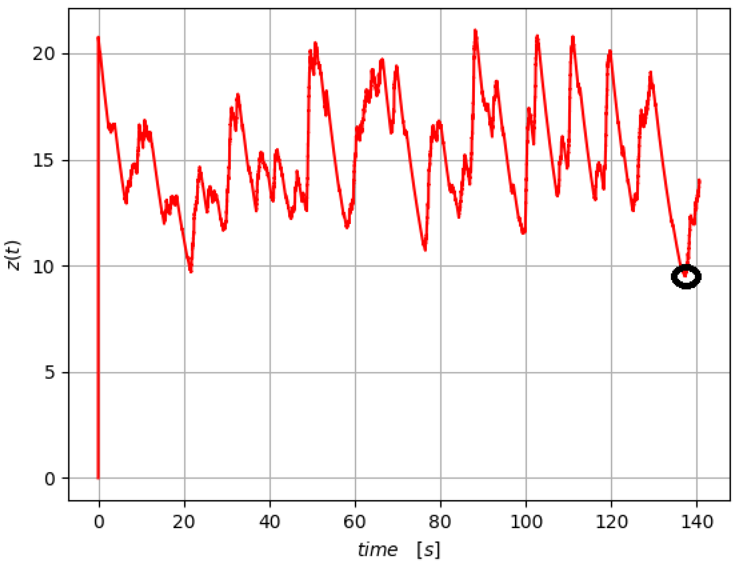
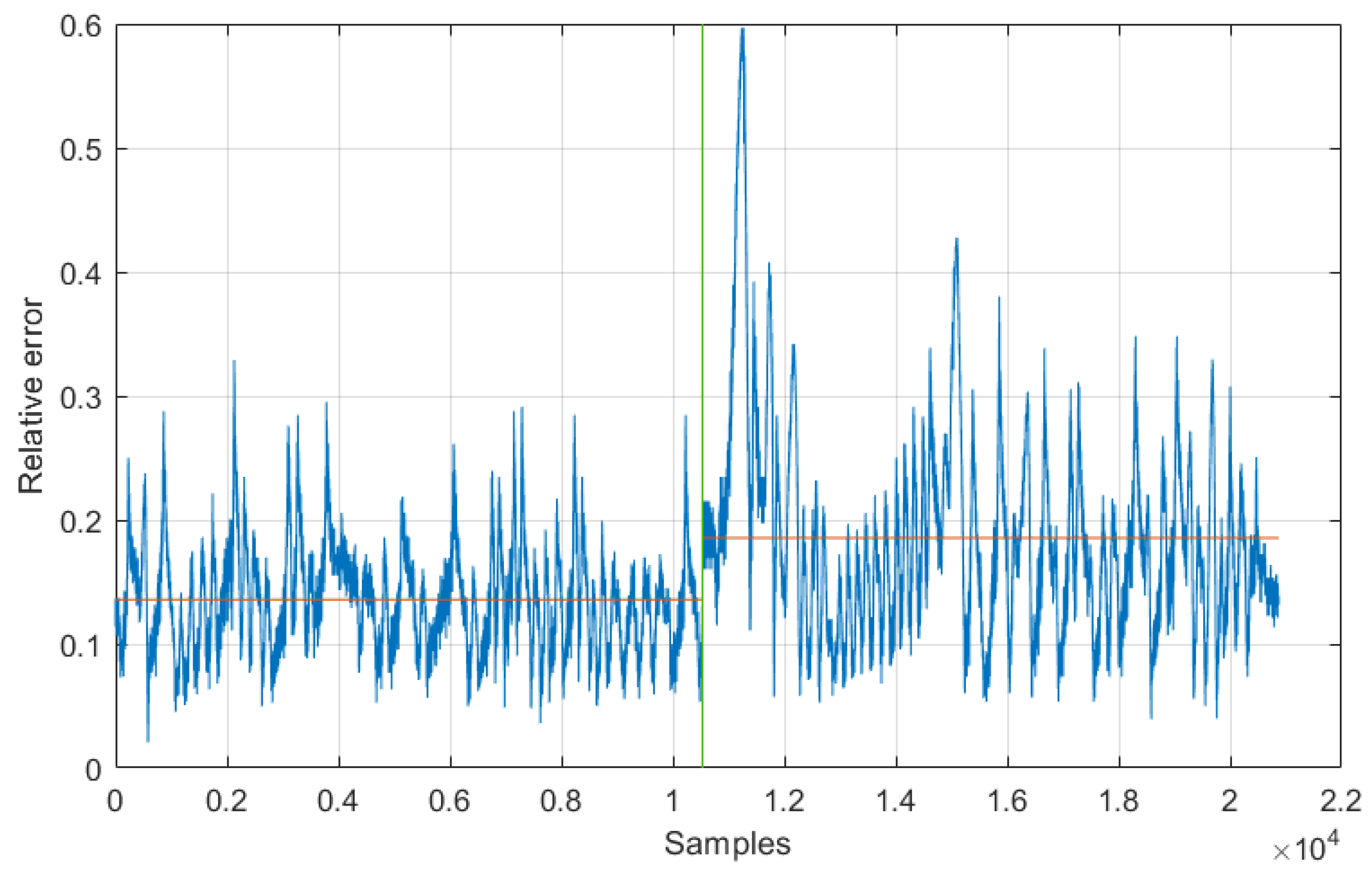
  • Obtain the experimental data series (within the series, the system can change status, as previously described).
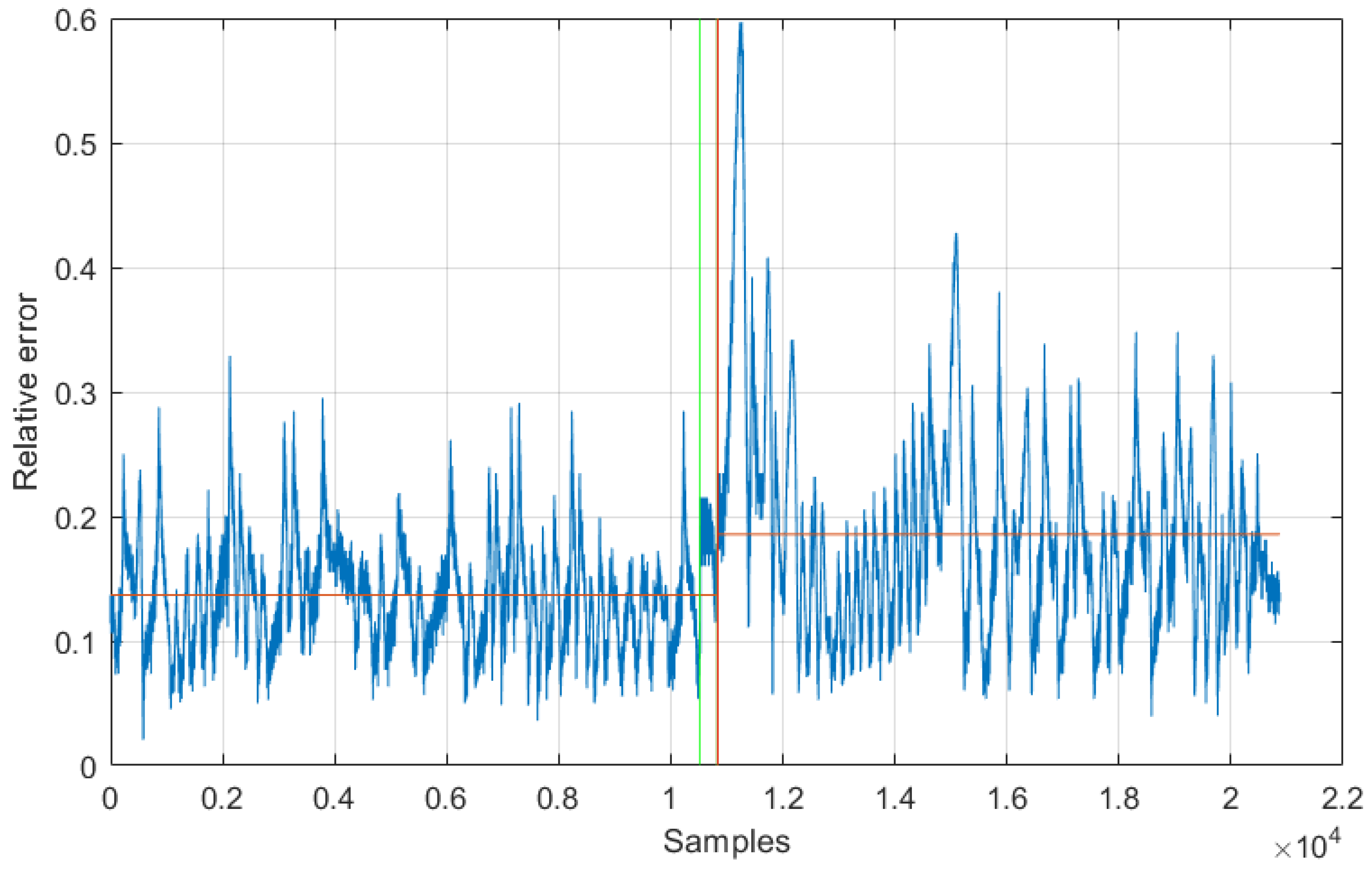
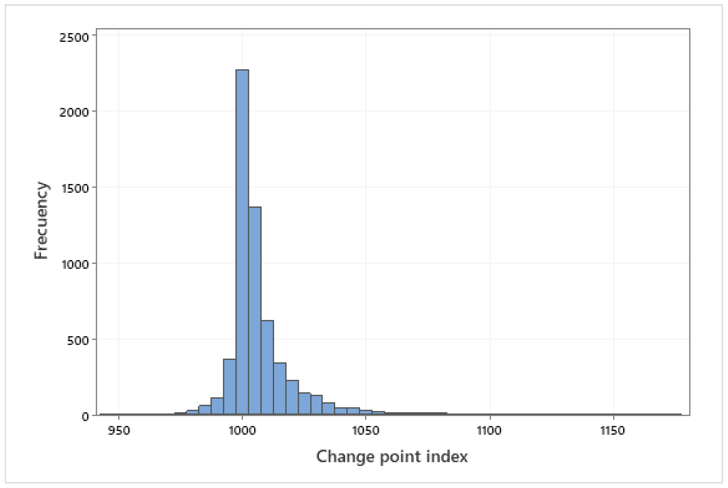
  • Minimize the index J ( k ) (15), using the arithmetic mean and the standard deviation, to detect the point of change:
    (a)
    Choose a point and divide the signal into two sections.
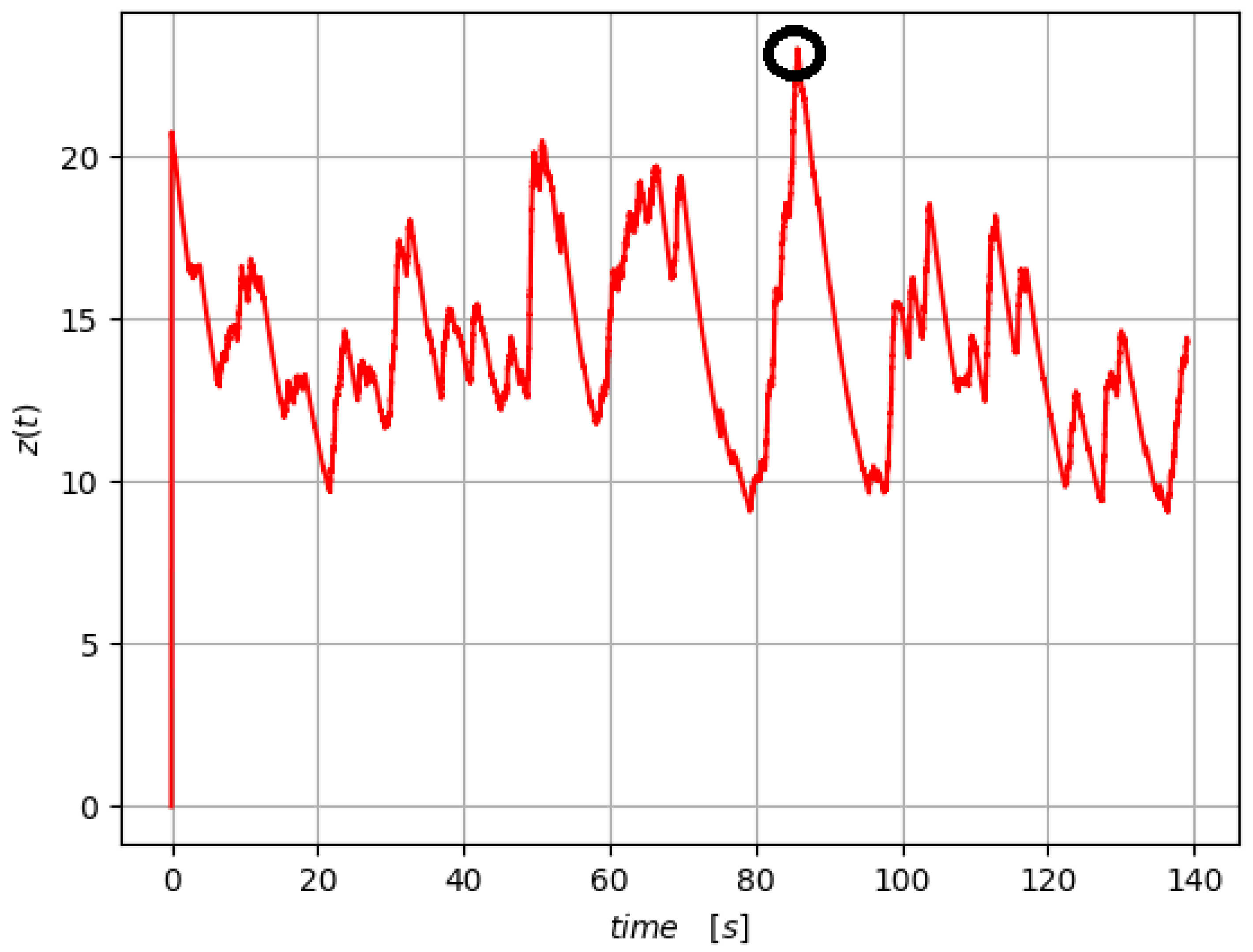
    (b)
    Compute an empirical estimate of the desired statistical property ( χ ) for each section.
    (c)
    At each point within a section, measure how much the property deviates from the empirical estimate. Add the deviations for all points.
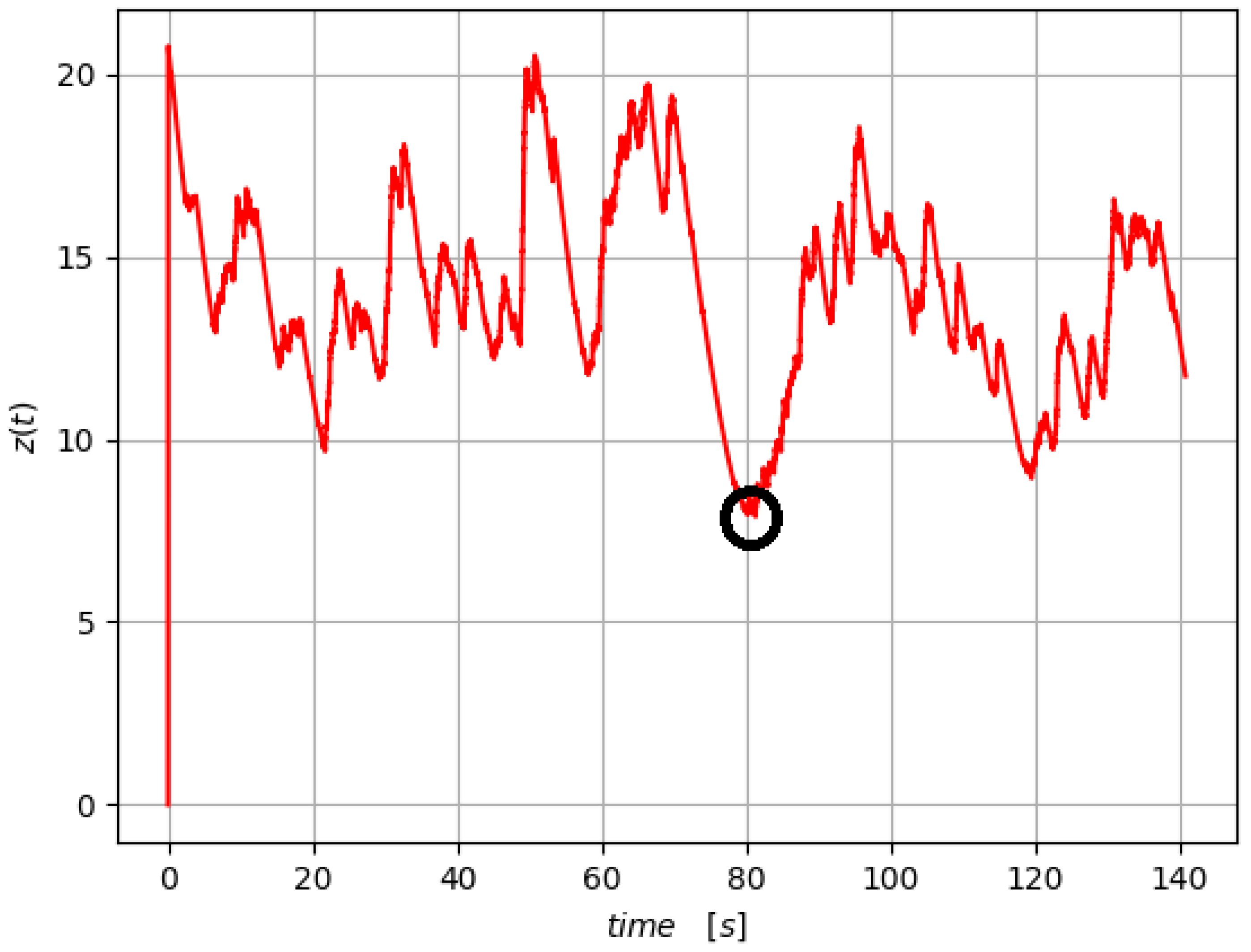
    (d)
    Add the deviations section to section to find the total residual error.
    (e)
    Vary the location of the division point until the total residual error attains a minimum.
  • The presence of a point of change detects a system fault and when it has happened.
In our case, to solve the second step, we use the MATLAB function “findchangepts” to find a point of change in an experimental data series [30,31].
Additionally, when only the trajectory error is studied, it is observed that the presence of faults can be detected (see Table 1). However a more precise technique must be used, and these errors infer that discrimination can be made. So, the main property of our load variation detection method lies in this discrimination: it allows to identify a point of change in a sample data, minimizing the index error.

4. Discussion

In this section we present first the good behavior of our method. Then, the accuracy of the fault detection algorithm is discussed, and finally compared to a deterministic one [29].

4.1. Validation: Experimental Study

In order to verify the detection of the system change point from normal to failure invoking our previous algorithm, we construct (concatenation of previous experimental data) the following three data series:
ε N 1 + ε F 1 , ε N 1 + ε F 2 , ε N 1 + ε F 3 .
In addition, the arithmetic mean and standard deviation statistics are used (local statistical parameter χ in (15)). To test our detection algorithm, based on CPD theory, the point of change must be detected and coincide with the change from normal to faulty case according to the data concatenation above. The results obtained are shown in Figure 22, Figure 23, Figure 24 and Figure 25.
For instance, Figure 22 shows 22,000 experimental data, where we know when a fault has occurred (register 10 527), and we want to test the performance of the algorithm presented in Section 3.3. Hence, by using the MATLAB function “findchangepts” [30], we solve step 2 of the algorithm, and find out the change of point at sample 10,527. So, we can detect the exact moment that a fault has occurred.
Figure 23 and Figure 24 also show the presence of load variation for ε N 1 + ε F 2 case. To see how the arithmetic mean and standard deviation works as CPD statistic parameter (15), the detection case ε N 1 + ε F 2 is studied in both cases. Figure 23 shows that the fault detection is achieved exactly. However, when standard deviation is considered (see Figure 24), a delay on the detection appears. This is due to the accuracy of the used method.
Case ε N 1 + ε F 3 is displayed in Figure 25, where again the arithmetic mean is considered, to be compared with the other two cases. In this case, again, a delay detection appears (the same result is obtained for the standard deviation).
In all cases, the test supports our approach: the real change of the experimental data series and the detection point of change are almost the same. So, the fault is detected and our algorithm shows good behavior.
The main advantage of our method, among the existing ones [6,7], is its simplicity and efficiency. After the designer obtains N samples, the data are processed, for example, by an easy-to-use MATLAB function, and a failure is observed, with minimized detection error. In addition, this method can be used to perform a test run of the wind turbine, for example, when we suspect ice accumulation on the blades. One drawback to be aware of is that real-time online fault detection cannot be performed in our approach. Additionally, due to the accuracy of the CPD method, in some cases, a delay data detection is appreciated (see Figure 25), but detection is almost always assured.

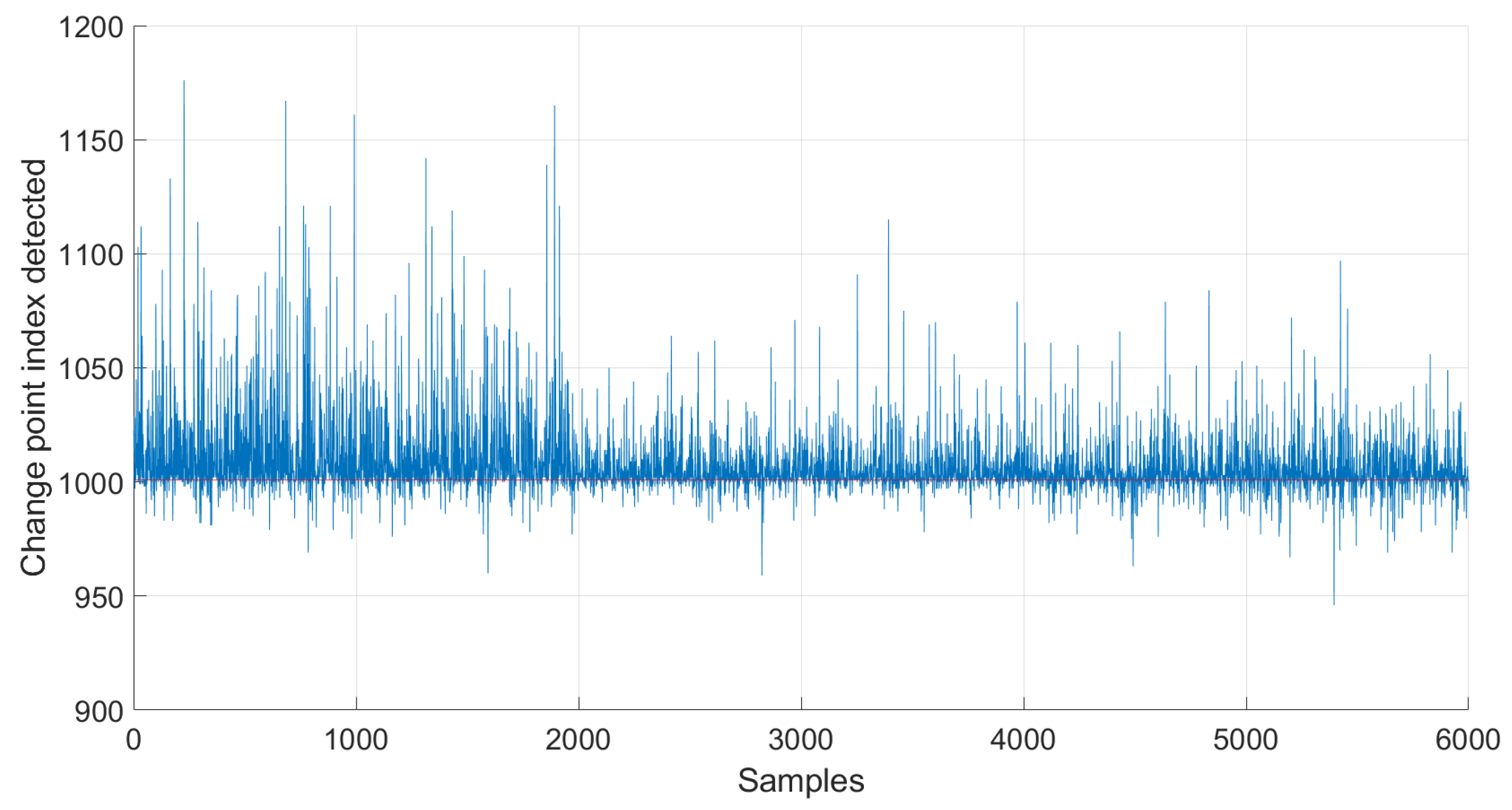
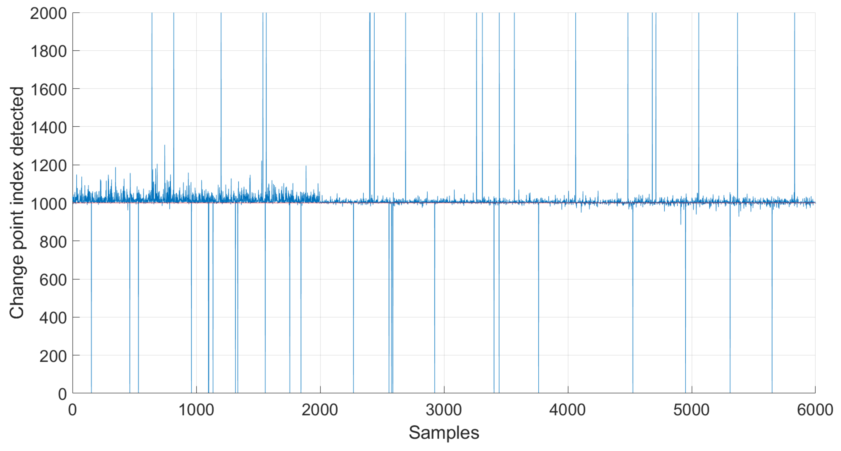
4.2. Accuracy Study of Fault Detection Algorithm

The objective of this section is to study the accuracy of the change point detection (CPD) method used in this work. From the experimental data obtained in Section 3.1, 6000 new series are randomly simulated: 2000 series corresponding to ε N 1 + ε F 1 , 2000 series corresponding to ε N 1 + ε F 2 and 2000 series corresponding to ε N 1 + ε F 3 . In all these series, the real point of change corresponds to the index 1001. The detection method of the point of change is applied to all of them, and the results are discussed below.
Figure 26 shows the point of change detected for each series, considering the arithmetic mean as the local statistical parameter in (15). To facilitate its interpretation, a histogram is shown (see Figure 27). It can be observed that the detected change point is found for the most part in the indices slightly higher than the real index of value 1001. Confidence intervals are calculated for the mean value of this index, obtaining an interval of (1006.81; 1007.58) for a 95 % confidence and (1006.69; 1007.70) for a 99 % confidence. That is, the failure is detected almost everywhere, with about 7 samples of delay. Considering the total among the experiments, we consider that our method presents good accuracy for detection.
We consider now the standard deviation as the local statistical parameter used in (15). Figure 28 shows the point of change detected for each series, in this case. Again, to facilitate its interpretation, a histogram is shown (Figure 29) in which it can also be observed that the point of change detected is mostly in the indices slightly higher than the real index equal to 1001. The confidence intervals are calculated for the value mean of this real index obtaining an interval of (1006.35; 1010.78) for a confidence of 95 % and (1005.65; 1011.47) for a confidence of 99 % . These values obtained slightly higher than 1001 show the goodness of the shift point detection method used in this work.
The first step in evaluating the performance of the change point method is to generate a confusion matrix that summarizes the actual and detected classes. There are four possibilities:
  • True positive (TP): there is a change point, and the algorithm detects it.
  • True negative (TN): there is no change point, and the algorithm does not detect anything.
  • False negative (FN): there is a change point, and the algorithm does not detect it.
  • False positive (FP): there is no change point, but the algorithm detects change.
To construct the confusion matrix, the 6000 simulated series with a real change point is considered, to which another 2000 series is added in which there is no change point. The results obtained are shown in the Table 2 and Table 3.
From the results shown in the Table 2 and Table 3, the following can be calculated:
  • Accuracy, calculated as the ratio of correctly classified data points to total data points. This measure provides a high-level idea about the algorithm’s performance:
    A c c u r a c y = T P + T N T P + F P + F N + T N .
  • Sensitivity, also referred to as recall or the true positive rate (TP Rate). This refers to the portion of a class of interest (change points) that was recognized correctly:
    S e n s i t i v i t y = T P T P + F N .
  • Precision. This is calculated as the ratio of true positive data points (change points) to total points classified as change points:
    P r e c i s i o n = T P T P + F P .
Table 4 shows the results obtained for this statistical parameters considering the arithmetic mean and the standard deviation as local parameters. It can be seen that the results show good performance, and the method can be used to discern a load variation on wind turbine. All measures are greater than 0.77 .
It should be noted that the proposed detection method has the worst precision among other existing methods. For example, Ref. [7] used a machine learning strategy to detect faulty behaviors, with a precision 10% which is better than our algorithm. However, the main advantage of our detection algorithm is its simplicity of implementation. This fact is an important objective when facing real experimentation, because the implementation becomes cheaper and able to produce an experimental platform for control and technology development.

4.3. Deterministic Diagnosis of Fault Detection

The main intention of this section is to offer a comparative method of a fault detection method to our approach. Because there are many methods today, we choose to use a common one from an engineering point of view in the deterministic systems set, especially the one described in Section 3.2. That is, we want to determine whether this system is capable of detecting load variations on the blade that will be reflected in the estimation of the time constant of the pitch system response. Therefore, and using the data described in Figure 22, Figure 23 and Figure 25, and using the same parametric estimation method described in Section 3.2, Figure 30, Figure 31 and Figure 32 show the result of the related experiment. They show the peak detector variable z ( t ) (13). Then, by using the healthy reference picture stated in Figure 14, and if we use the threshold method, the peak values are detected (marked in black circles in the cited Figures) indicating a fault [29]. It can be observed that due to the behavior of the experiment, the failures cannot be well observed. Therefore, the adaptive method can hardly detect a fault, but our approach does.

5. Conclusions and Future Work

This article proposes an efficient digital proportional controller and a faulty detection scheme to monitor load variations on an experimental platform. This platform emulates load variations on the blades of a wind turbine. In addition, a new experimental setup was created to simulate load variation on the blade of a wind turbine by using a throttle device and its electrical model. Note that the wind turbine under consideration was a large three-bladed horizontal axis wind turbine with its blades positioned upwind from the tower. Then, baed on a series of experimental data, there is a growing need to be able to detect changes in the distribution properties of those data over time and look for these changes efficiently. Obviously, these changes occur, for example, due to a possible failure of the system that produces them. In many current shift point detection problems, researchers focus their efforts on the conjecture that the number of shift points is expected to increase as the series increases in number of data. In our approach, only the first change point is needed to detect the instant of system failure. Consequently, the appropriate statistical methodology of the change point detection (CPD) method was applied to the series of experimental data provided by the experimental platform. The experimental results support our approach to detecting load variation in the blades of a wind turbine. Moreover, a static point of change in the experimental data was used to detect this load variation, where a large statistical difference was detected. Its novelty is based on the direct study of data, obtaining an efficient fault detection algorithm. Consequently, a discrimination rule is established, using the shift point methodology.
Finally, as future work, a more complex wind turbine (WT) can be considered, for example, the floating offshore one, with different load dynamics from that considered in the present work [32]. In this case, the controller must be improved to cope with these new dynamics. However, we consider that the proposed fault detection algorithm can also be useful in this case too.

Author Contributions

Conceptualization, L.A.; methodology, G.P.-V., J.G.-B. and P.B.; software, J.G.-B., L.A. and P.B.; validation, L.A., G.P.-V., J.G.-B. and P.B.; formal analysis, J.G.-B.; investigation, L.A., G.P.-V., J.G.-B. and P.B.; resources, L.A. and J.G.-B.; data curation, J.G.-B. and P.B.; writing—original draft preparation, L.A.; writing—review and editing, L.A., G.P.-V., J.G.-B. and P.B.; visualization, L.A., G.P.-V., J.G.-B. and P.B.; supervision, L.A., G.P.-V. and J.G.-B.; project administration, G.P.-V.; funding acquisition, L.A. All authors have read and agreed to the published version of the manuscript.

Funding

This research received no external funding.

Institutional Review Board Statement

Not applicable.

Informed Consent Statement

Not applicable.

Data Availability Statement

Data sharing not applicable.

Conflicts of Interest

The authors declare no conflict of interest. The funder had no role in the design of the study; in the collection, analyses, or interpretation of data; in the writing of the manuscript; or in the decision to publish the results.

Abbreviations

The following abbreviations are used in this manuscript:
CPDChange Point Detection
PICProgrammable Integrated Circuit
TPTrue Positive
TNTrue Negative
FPFalse Positive
FNFalse Negative
WTWind Turbine

Appendix A. C-Program and Micro-Controller Settings

In order to facilitate the reproduction of the experiment, we present in Figure A1 and Figure A2 the program used to perform the experiments. First, the internal specifications are defined. Then the two voltage reading channels CH0 and CH1 are assigned, allowing the micro-controller (7) to be defined. Note that its analog version corresponds to (8). Finally, a time delay is considered to avoid data read overlapping.
Figure A1. Main part of the C-program, where the proportional controller (8) is defined (to be continued on the next figure).
Energies 15 00568 g0a1
Figure A2. Here, the input and output variables are defined, along with the time-delay mandatory to avoid overlapping readings by the micro-controller unit (symbol /*text*/ is used to add a comment).
Energies 15 00568 g0a2

References

  1. Njiri, J.G.; Beganovic, N.; Do, M.H.; Söffker, D. Consideration of lifetime and fatigue load in wind turbine control. Renew. Energy 2019, 131, 818–828. [Google Scholar] [CrossRef]
  2. Habibi, H.; Howard, I.; Simani, S. Reliability improvement of wind turbine power generation using model-based fault detection and fault tolerant control: A review. Renew. Energy 2019, 135, 877–896. [Google Scholar] [CrossRef]
  3. Du, Y.; Zhou, S.; Jing, X.; Peng, Y.; Wu, H.; Kwok, N. Damage detection techniques for wind turbine blades: A review. Mech. Syst. Signal Process. 2020, 141, 1–23. [Google Scholar] [CrossRef]
  4. Yang, B.; Sun, D. Testing, inspecting and monitoring technologies for wind turbine blades: A survey. Renew. Sustain. Energy Rev. 2013, 22, 515–526. [Google Scholar] [CrossRef]
  5. Dong, X.; Gao, D.; Li, J.; Jincao, Z.; Zheng, K. Blades icing identification model of wind turbines based on SCADA data. Renew. Energy 2020, 162, 575–586. [Google Scholar] [CrossRef]
  6. Liu, Z.; Zhang, L. A review of failure modes, condition monitoring and fault diagnosis methods for large-scale wind turbine bearings. Measurement 2020, 149, 107002. [Google Scholar] [CrossRef]
  7. Tong, R.; Lia, P.; Lang, X.; Liang, J.; Cao, M. A novel adaptive weighted kernel extreme learning machine algorithm and its application in wind turbine blade icing fault detection. Measurements 2021, 185, 110009. [Google Scholar] [CrossRef]
  8. Pujol-Vazquez, G.; Acho, L.; Gibergans-Báguena, J. Fault Detection Algorithm for Wind Turbines Pitch Actuator Systems. Energies 2020, 13, 2861. [Google Scholar] [CrossRef]
  9. Vidal, Y.; Tutivén, C.; Rodellar, J.; Acho, L. Fault diagnosis and fault-tolerant control of wind turbines via a discrete time controller with a disturbance compensator. Energies 2015, 8, 4300–4316. [Google Scholar] [CrossRef] [Green Version]
  10. Ruiz, M.; Mujica, L.E.; Alferez, S.; Acho, L.; Tutiven, C.; Vidal, Y.; Pozo, F. Wind turbine fault detection and classification by means of image texture analysis. Mech. Syst. Signal Process. 2018, 107, 149–167. [Google Scholar] [CrossRef] [Green Version]
  11. Xu, Q.; Fan, Z.; Jia, W.; Jiang, C. Fault detection of wind turbines via multivariate process monitoring based on vine copulas. Renew. Energy 2020, 161, 939–955. [Google Scholar] [CrossRef]
  12. Ohishi, K.; Nakao, M.; Ohnishi, K.; Miyachi, K. Microprocessor-controlled DC motor for load-insensitive position servo system. IEEE Trans. Ind. Electron. 1987, 1, 44–49. [Google Scholar] [CrossRef]
  13. Acho, L. A proportional plus a hysteretic term control design: A throttle experimental emulation to wind turbines pitch control. Energies 2019, 12, 1961. [Google Scholar] [CrossRef] [Green Version]
  14. Shajiee, S.; Pao, L.Y.; McLeod, R.R. Monitoring ice accumulation and active de-icing control of wind turbine blades. In Wind Turbine Control and Monitoring; Springer: Cham, Switzerland, 2014; pp. 193–230. [Google Scholar]
  15. Yun, H.; Zhang, C.; Hou, C.; Liu, Z. An Adaptive Approach for Ice Detection in Wind Turbine With Inductive Transfer Learning. IEEE Access 2019, 7, 122205–122213. [Google Scholar] [CrossRef]
  16. Aminikhanghahi, S.; Cook, D.J. A Survey of Methods for Time Series Change Point Detection. Knowl. Inf. Syst. 2017, 51, 339–367. [Google Scholar] [CrossRef] [Green Version]
  17. Page, E.S. Continuous Inspection Schemes. Biometrika 1954, 41, 100–115. [Google Scholar] [CrossRef]
  18. Gallagher, C.; Lund, R.; Robbins, M. Changepoint Detection in Climate Time Series with Long-Term Trends. J. Clim. 2013, 26, 4994–5006. [Google Scholar] [CrossRef]
  19. Mudelsee, M. Trend analysis of climate time series: A review of methods. Earth-Sci. Rev. 2019, 190, 310–322. [Google Scholar] [CrossRef]
  20. You, S.H.; Jang, E.J.; Kim, M.S.; Lee, M.T.; Kang, Y.J.; Lee, J.E.; Eom, J.H.; Jung, S.Y. Change Point Analysis for Detecting Vaccine Safety Signals. Vaccines 2021, 9, 206. [Google Scholar] [CrossRef] [PubMed]
  21. Militino, A.F.; Moradi, M.; Ugarte, M.D. On the Performances of Trend and Change-Point Detection Methods for Remote Sensing Data. Remote Sens. 2020, 12, 1008. [Google Scholar] [CrossRef] [Green Version]
  22. Borsoi, R.; Richard, C.; Ferrari, A.; Chen, J.; Bermudez, J.M. Online graph-based change point detection in multiband image sequences. In Proceedings of the 28th European Signal Processing Conference (EUSIPCO), Amsterdam, The Netherlands, 18–21 January 2021; pp. 850–854. [Google Scholar]
  23. Taylor, S.J.; Letham, B. Forecasting at Scale. Am. Stat. 2018, 72, 37–45. [Google Scholar] [CrossRef]
  24. Killick, R.; Fearnhead, P.; Eckley, I.A. Optimal Detection of Changepoints with a Linear Computational Cost. J. Am. Stat. Assoc. 2012, 197, 1590–1598. [Google Scholar] [CrossRef]
  25. Truong, C.; Oudre, L.; Vayatis, N. Selective review of offline change point detection methods. Signal Process. 2019, 197, 107299. [Google Scholar] [CrossRef] [Green Version]
  26. Usman, H.M.; Mukhopadhyay, S.; Rehman, H. Permanent magnet DC motor parameters estimation via universal adaptive stabilization. Control Eng. Pract. 2019, 90, 50–62. [Google Scholar] [CrossRef]
  27. Bates, M. PIC Microcontrollers: An Introduction to Microelectronics, 2nd ed.; Newnes: Burlington, WA, USA, 2004; p. 215. [Google Scholar]
  28. Inthamoussou, F.A.; Bianchi, F.D.; De Battista, H.; Mantz, R.J. Gain Scheduled H- Control of Wind Turbines for the Entire Operating Range. In Wind Turbine Control and Monitoring; Springer: Cham, Switzerland, 2014; pp. 71–95. [Google Scholar] [CrossRef]
  29. Acho, L.; Pujol, G. A boundary control technique to the string-tip-mass system based on a non-symmetric peak-detector model. In Proceedings of the 2017 21st International Conference on System Theory, Control and Computing (ICSTCC), Sinaia, Romania, 19–21 October 2017; pp. 759–762. [Google Scholar] [CrossRef]
  30. Caulcutt, R. Statistics in Research and Development; Chapman and Hall/CRC: Boca Raton, FL, USA, 2019; ISBN 9780367450472. [Google Scholar]
  31. Matlab, Signal Processing Toolbox Reference, 1988–2021 The MathWorks, Inc. Available online: https://www.mathworks.com/ (accessed on 20 December 2021).
  32. Cai, C.; Maeda, T.; Kamada, Y.; Wang, X.; Zhou, S.; Zhang, F. Wind tunnel and numerical study of a floating offshore wind turbine based on the cyclic pitch control. Renew. Energy 2021, 172, 453–464. [Google Scholar] [CrossRef]
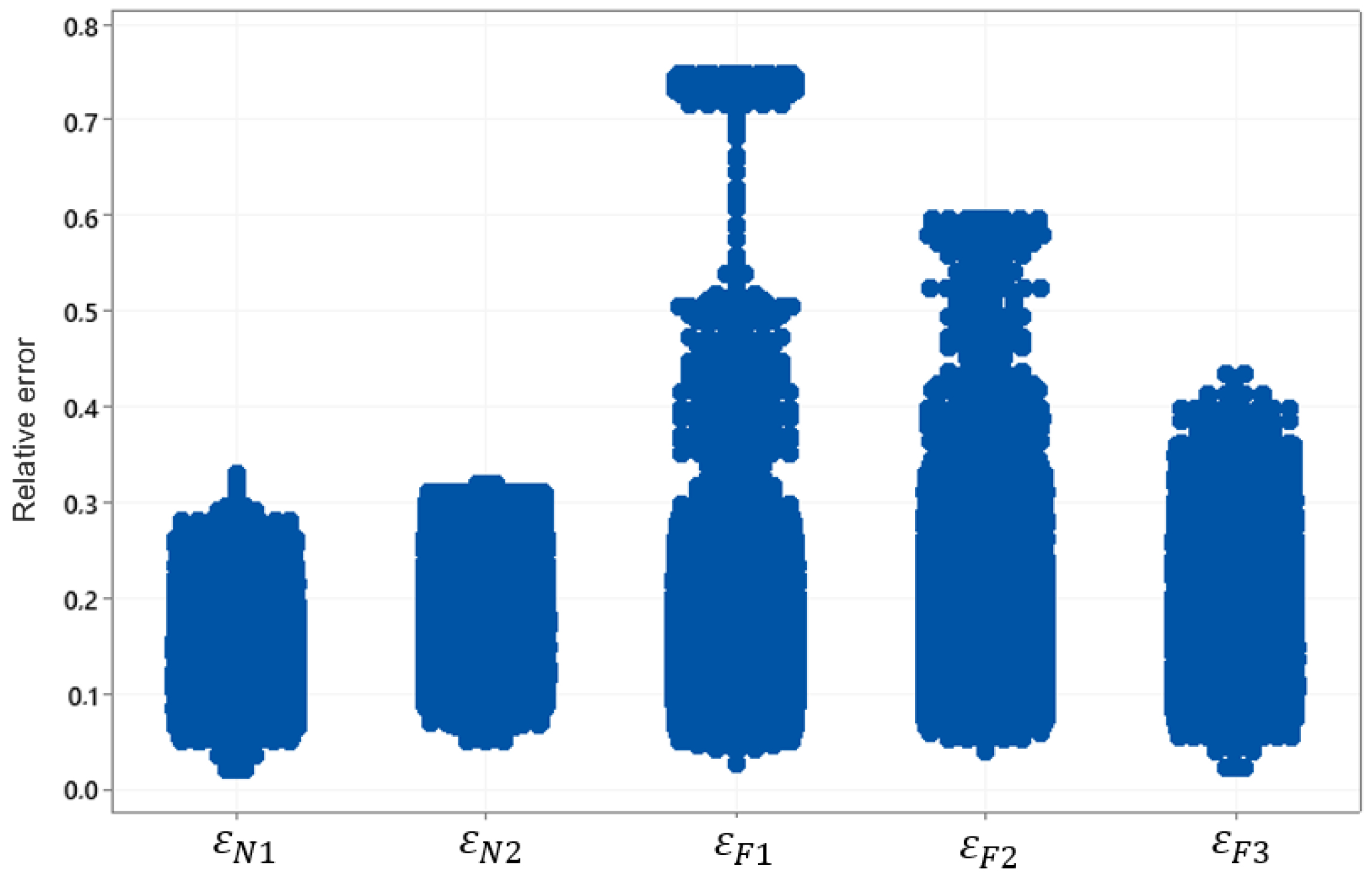
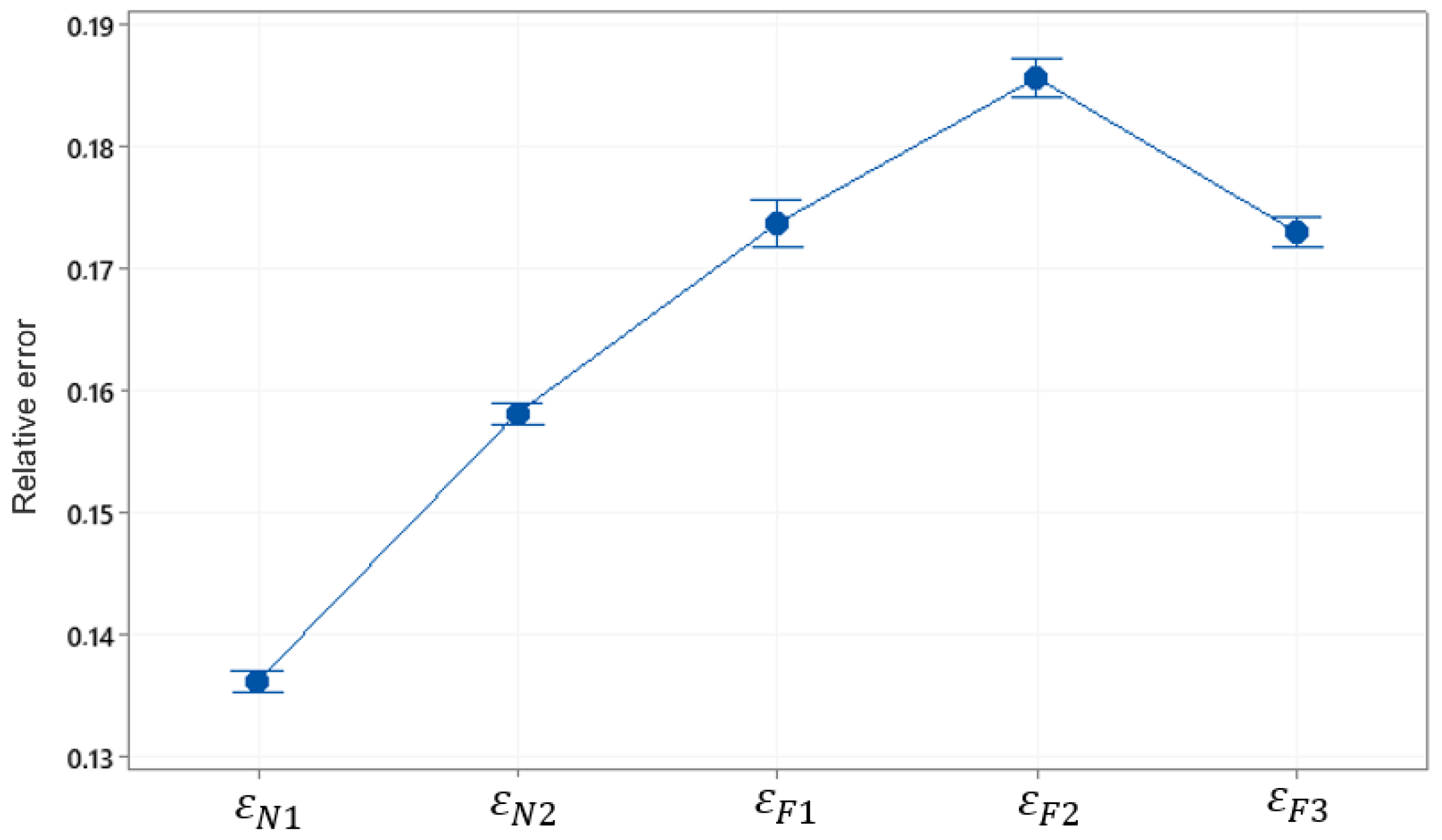
Figure 1. An overview of the main parts of a wind turbine, including its pitch system (the above figures are with the Creative Commons Attribution 4.0 International License).
Energies 15 00568 g001
Figure 2. A schematic of an automotive throttle valve [13]. Compared to Figure 1, it can be seen that both have a similar gearbox system. Here, the throttle return spring corresponds to the presence of load on the blades of a wind turbine.
Energies 15 00568 g002
Figure 3. An overview of the closed-loop pitch system with a controller. β and β r e f are the pitch angle and the pitch reference command, respectively.
Energies 15 00568 g003
Figure 4. A photo of the realized experimental platform, composed by a throttle device, the reference signal manually commanded, and the electronic circuit along with the micro-controller. The resistance R d allows to emulate load variations. See a video on experimentation at https://youtu.be/Bi6zsrT9yyY (accessed date: 20 May 2021).
Energies 15 00568 g004
Figure 5. Electromagnetic representation of a (permanent) DC-motor system. The proportional controller, u ( t ) , defined by the micro-controller, is the motor input variable. The internal variables of the throttle device (current i a , motor resistance R a , inductance L a , force constant K b w ( t ) , motor load J, viscous friction b) define the mathematical model (1) and (2). Additionally, this scheme includes the external resistance R d , the emulator of the load variation on a wind turbine.
Energies 15 00568 g005
Figure 6. Electronic circuit. The power transistors are MJE3055T and MJE2955T for Q 1 and Q 2 , respectively. The potentiometer (trimmer) P 1 supplies the reference command which is manually manipulated, and P 2 comes from the throttle plate sensor. The permanent DC motor of the throttle mechanism is shown too. The switch S W 1 activates the master clear enable of the micro-controller (the external reset to the digital device).
Energies 15 00568 g006
Figure 7. Blocks diagram of the electronic design. The Picoscope 2000 series is used to read data from the computer. This device is widely used in data acquisition with high precision.
Energies 15 00568 g007
Figure 8. Throttle sensor response.
Energies 15 00568 g008
Figure 9. Case N 1 : Experimental results with R d = 0 ohms, showing the throttle angle β and reference signal β r e f .
Energies 15 00568 g009
Figure 10. Case N 2 : Other experimental results with R d = 0 ohms, showing the throttle angle β and reference signal β r e f .
Energies 15 00568 g010
Figure 11. Case F 1 : Experimental results with R d = 0.5 ohms, displaying the throttle angle β and reference signal β r e f .
Energies 15 00568 g011
Figure 12. Case F 2 : Other experimental results with R d = 0.5 ohms, drawing the throttle angle β and reference signal β r e f .
Energies 15 00568 g012
Figure 13. Case F 3 : Another experimental results with R d = 0.5 ohms, marking the throttle angle β and reference signal β r e f .
Energies 15 00568 g013
Figure 14. Observer response z ( t ) . Here, τ = 0.01 , α = 10 , γ = 0.1 , and θ * = 1 .
Energies 15 00568 g014
Figure 15. Case N 1 : Relative error ε N 1 (14), for the nominal experiment with R d = 0 ohms.
Energies 15 00568 g015
Figure 16. Case N 2 : Relative error ε N 2 (14), for the nominal experiment with R d = 0 ohms.
Energies 15 00568 g016
Figure 17. Case F 1 : Relative error ε F 1 (14), for the faulty experiment with R d = 0.5 ohms.
Energies 15 00568 g017
Figure 18. Case F 2 : Relative error ε F 2 (14), for the faulty experiment with R d = 0.5 ohms.
Energies 15 00568 g018
Figure 19. Case F 3 : Relative error ε F 3 (14), for the faulty experiment with R d = 0.5 ohms.
Energies 15 00568 g019
Figure 20. Dot plots of the five series of relative errors, where the discrimination between nominal and faulty cases can be appreciated. Therefore, this suggests that the change point detection method [16] can be used to discriminate faults.
Energies 15 00568 g020
Figure 21. Boxplots of the five relative error series.
Energies 15 00568 g021
Figure 22. Detection of point of change in series ε N 1 + ε F 1 considering the arithmetic mean as a local statistical parameter. The real change is in register 10,527 and the CPD is in register 10,527 (green vertical line), obtaining an exact detection. The same result is obtained considering the standard deviation as a local statistical parameter.
Energies 15 00568 g022
Figure 23. Detection of point of change in series ε N 1 + ε F 2 considering the arithmetic mean as a local statistical parameter. The real change is in register 10,527 and the CPD is in register 10,527 (green vertical line).
Energies 15 00568 g023
Figure 24. Detection of point of change in series ε N 1 + ε F 2 considering the standard deviation as a local statistical parameter. The real change is in register 10,527 (green vertical line) and the CPD is in register 10,829 (red vertical line).
Energies 15 00568 g024
Figure 25. Detection of point of change in series ε N 1 + ε F 3 considering the mean as a local statistical parameter. The real change is in register 10,527 (green vertical line) and the CPD is in register 10,933 (red vertical line). The same result is obtained considering the standard deviation as a local statistical parameter.
Energies 15 00568 g025
Figure 26. Plot of the points of change detected considering the arithmetic mean as the local statistical parameter used, corresponding to the 6000 simulated series. For most of them, the change point occurs close to 1001, as expected.
Energies 15 00568 g026
Figure 27. Histogram of the change point detected for the 6000 simulated series, considering the arithmetic mean as the local statistical parameter used. The real change occurs at sample 1001, where the data are accumulated.
Energies 15 00568 g027
Figure 28. Plot of the points of change detected considering the standard deviation as the local statistical parameter used, corresponding to the 6000 simulated series.
Energies 15 00568 g028
Figure 29. Histogram of the change point detected for the 6000 simulated series considering the standard deviation as the local statistical parameter used, showing a good accuracy of the CPD method.
Energies 15 00568 g029
Figure 30. Parametric estimation case 1: ε N 1 + ε F 1 serie.
Energies 15 00568 g030
Figure 31. Parametric estimation case 2: ε N 1 + ε F 2 serie.
Energies 15 00568 g031
Figure 32. Parametric estimation case 3: ε N 1 + ε F 3 serie.
Energies 15 00568 g032
Table 1. Statistical summary of the series under study.
VariableNMeanStdMin Q 1 Q 2 Q 3 Max
ε N 1 10,5260.136220.042620.020760.104560.133080.160680.32907
ε N 2 10,5050.158130.046360.049980.121790.148960.181320.31979
ε F 1 10,5680.173630.099970.026310.117800.159730.196750.74766
ε F 2 10,3440.185530.083850.039560.131280.172520.219890.59667
ε F 3 10,5960.172940.061970.022450.128300.168260.206160.43353
Table 2. Confusion matrix obtained for the 6000 simulated series considering the arithmetic mean as the local statistical parameter used in the CPD algorithm.
Change Point DetectedNon-Change Point Detected
True change point V P = 4848 T P = 556
True non-change point T N = 1280 V N = 1316
Table 3. Confusion matrix obtained from the 6000 simulated series and by considering the standard deviation as the local statistical parameter used in our the CPD algorithm.
Change Point DetectedNon-Change Point Detected
True change point V P = 4994 T P = 466
True non-change point T N = 1070 V N = 1470
Table 4. Performance metrics employed to evaluate CPD algorithm, considering the arithmetic mean and the standard deviation as local parameters.
Arithmetic MeanStandard Deviation
Accuracy 0.7705 0.8080
Sensitivity 0.7911 0.8235
Precision 0.8971 0.9146
Publisher’s Note: MDPI stays neutral with regard to jurisdictional claims in published maps and institutional affiliations.

