Abstract
Gas–liquid flow in a pipeline is a very common. Slug two-phase flow is dominated in the case of slightly upward flow (+0.25°) and considered to be the comprehensive flow configuration, and can be in close contact with all the other flow patterns. The models of different flow patterns can be unified. Precise prediction of the slug flow is crucial for proper design and operation. In this paper, we develop hydrodynamics unified modeling for gas–liquid two-phase slug flow, and the bubble and droplet entrainment is optimized. For the important parameters (wall and interfacial friction factors, slug translational velocity and average slug length), the correlations of these parameters are optimized. Furthermore, the related parameters for liquid droplet and gas bubble entrainment are given. Accounting for the gas–liquid interface shape, hydrodynamics models, i.e., the flat interface model (FIM) and the double interface model (DIM), of liquid film in the slug body are applied and compared with the experimental data. The calculated results show that the predictions for the liquid holdup and pressure gradient of the DIM agree with experimental data better than those of the FIM. A comparison between the available experimental results and Zhang’s model calculations shows that the DIM model correctly describes the slug dynamics in gas–liquid pipe flow.
1. Introduction
Gas–liquid flow in a pipeline is very common. Due to its remarkable economic benefit, it has been applied widely in geothermal fields, oil and gas industries, chemical reactors, nuclear reactors, aerosols, and various other heat and mass transfer processes during the past 40 years [1,2,3,4]. Slug two-phase flow is dominated in the case of slightly upward flow (+0.25°) and considered to be the comprehensive flow configuration [5,6]. It can be in close contact with all other flow patterns; for example, the liquid film zone of the slug unit is similar to that of stratified flow, and the liquid slug body resembles that of bubbly or dispersed bubble flow [7,8]. Thus, the study of the slug flow can also capture the behaviors of the other flow patterns [9,10].
To optimize oil and gas production and transportation, flow behaviors such as flow pattern, liquid holdup, and pressure gradient need to be predicted accurately. Early models to predict gas–liquid hydrodynamic characteristics were based on empirical correlations [11,12,13]. The application of empirical correlations simplifies the complex physics and limits the opportunity to improve the models. The empirical correlations of liquid holdup and pressure drop scaled up to oilfield applications are inaccurate, because these correlations are obtained from small-scale laboratory data.
Recently, mechanistic models were proposed to overcome this problem. Spedding et al. [14] developed a slug flow specification model to describe the slug initiation, growth, and decay, and tested 60 models on the basis of the 12 possible flow regimes. Bendiksen et al. [15] incorporated a unit-cell type of slug flow description into the transient two-fluid model for the simulation of two-phase oil and gas flow in pipelines, and predictions of liquid holdup and pressure gradient were found to agree with experimental data. De Henau and Raithby [16,17] developed a one-dimensional transient two-fluid model with slug flow, which provides the necessary interphase constitutive relations for the drag coefficient and the parameters for the closure relations incorporated in the momentum conservation equations. Issa and Kempf [18] proposed a mechanistic one-dimensional model to predict hydrodynamic slug formation, growth, and decay, and the subsequent development of the slug shape into continuous slug flow, based on the numerical solution of the one-dimensional transient two-fluid model equations. The results of computations for the slug characteristics were considered to be in agreement with results of the experiments. Losi et al. [19] experimentally and theoretically investigated high viscosity oil–air slug flow, and built probability density functions for slug lengths based on superficial gas velocity. Arabi et al. [20] experimentally investigated the slug frequency of intermittent air–water flow in a horizontal pipe, investigated the influence of the sub-regime on slug frequency, and developed a new slug frequency correlation for intermittent flow.
Gas–liquid two-phase slug flow has been investigated continuously in previous studies, partially because of its complexity. Every other flow pattern can be represented in slug flow, e.g., the film zone of slug flow resembles that of stratified or annular flow, and the slug body resembles that of bubbly or dispersed bubble flow [7]. Zhang et al. [7,21] developed a unified model for gas–liquid pipe flow via slug dynamics. The relationship of each flow pattern can be obtained, through the transformation of the slug flow relationship, so as to achieve the unification of the calculation model for each flow pattern. However, although the model describes the phenomenon of gas–liquid entrainment, its processing method is too simple, and only considers the entrainment fraction of the two parameters of droplet and gas holdup. In fact, entrainment of droplets and bubbles occurs only under certain conditions. Furthermore, there is still a limited amount of information about the influence of the gas–liquid interface shape in slug flow hydrodynamics. A good description of interface shape is important when examining the liquid film zone of the slug unit in slug flow. Three typical interface configurations of stratified flow are presented in the literature: the flat interface model, the apparent rough surface model, and the concave down configuration. In the current study, a new mechanistic model was formulated and tested against experimental data, based on the comparison of these three interface configurations.
2. Hydrodynamic Model
The hydrodynamics model was derived for fully developed hydraulic gas–liquid slug flow, where there is no heat and mass transfer between gas and liquid phases. The continuity, momentum, and equations of slug flow were established by taking the liquid film region as the control volume. The momentum equation of slug flow can be transformed into the equation of stratified flow after the momentum exchange term is eliminated. The annular flow momentum equation can be obtained when the friction term of the gas wall is eliminated. The basic equations of each flow pattern are unified.
Some assumptions are required because of the gas–liquid slug flow complexity: a fully developed slug flow, and negligible momentum exchange between the liquid slug and the liquid film.
2.1. Slug Flow
2.1.1. Continuity Equation
The slug unit is defined as the control volume for the fully developed slug flow, as shown in Figure 1, including the entire liquid film zone and the gas pocket (liquid slug) zone.
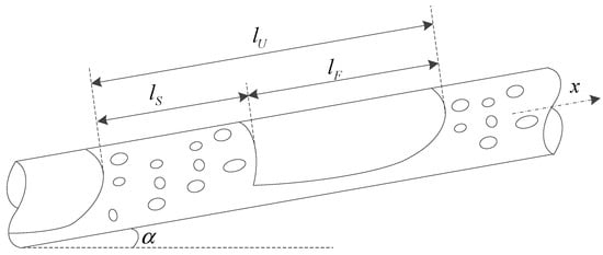
Figure 1.
Control volume for the slug unit.
The liquid slug zone included in the liquid occupies the entire pipe cross-section containing the bubble. The liquid film including the liquid film and gas pocket (i.e., a Taylor bubble) is in close proximity to the liquid slug zone. , , and are lengths of the slug unit, liquid slug zone, and liquid film zone, respectively.
The length of slug unit is defined as:
Considering the passage of a slug unit at an observation point, the following relationships hold for the liquid and gas phases, respectively:
Considering the entrainment of liquid droplets in the gas core, the gas continuity equation can be obtained by taking two cross-sections of the liquid film and liquid slug regions:
where , , , and are velocities of the slug unit, liquid film, gas pocket, and gas–liquid mixture in the liquid slug, respectively. , and are liquid holdups in the slug body, film, and liquid slug, respectively:
For a fully developed slug flow, the slug translational velocity refers to the velocity of the slug front (or the head of the long bubble). One of the key issues for hydrodynamic slug flow is the slug front velocity (or slug bubble velocity); this is one of the governing parameters for the modeling of hydrodynamic slug flow:
where is the drift velocity. It is calculated according to:
where is the empirical coefficient of speed distribution; for a fully developed pipeline cross-section speed distribution, is approximately equal to the ratio of maximum speed to average speed. When the gas–liquid mixture in the liquid plug is sufficiently turbulent, . When the gas–liquid mixture in the liquid plug is laminar flow, .
The liquid holdup in liquid slug, , is given as:
Following the same derivation as the gas phase, the continuity equation of the liquid phase can be written as:
Adding Equation (4) to Equation (13):
where .
where and are superficial velocities of liquid and gas: , .
The volume difference generated by the difference velocity between the gas pocket and liquid slug in liquid film zone is defined as , and the volume difference generated by the difference velocity between liquid film and liquid slug is defined as . Volume differences and are equal, due to being inside the slug body, so:
According the Equations (2), (3), (4), (13), and (16), , , , , and can be written as:
2.1.2. Momentum Equation
The liquid film and gas pocket in the film zone are separately used as the control volumes for the derivation of momentum equations. For fully developed slug flow, the momentum exchanges per unit time between the slug body and liquid film in the direction of the frictional and gravitational forces acting on the film are in balance. The liquid and gas phase momentum equations are written as:
Equating the pressure drop of the gas and liquid phase and subtracting Equation (23) from Equation (22) gives:
Eliminating in both Equation (22) and Equation (23) gives:
The liquid slug momentum equation is written as:
i.e.,
where , .
Equation (27) can be given as:
The momentum transfer term between the liquid plug region and the liquid film region does not appear in the Equation (28). However, the momentum transfer between the two regions affects the slug flow characteristics.
2.2. Stratified and Annular Flows
The momentum equation for stratified flow is obtained by removing the momentum exchange terms from Equation (28), given as:
In annular flow, there is no contact between the gas core and the pipe wall. Equation (28) then becomes:
2.3. Bubble Flow
Bubble flow includes dispersed bubble flow and bubble flow. The liquid holdup and pressure gradient of dispersed bubble flow are calculated when it is assumed that the gas–liquid mixture is uniform. For bubbly flows, the rate of bubble rise relative to the liquid must be considered; , is estimated by the Harmathy correlation:
3. Closure Relationships
The implementation of the model is dependent on both the basic equations and closure relationships. The wall friction factor, interfacial friction factor, slug length, and slug liquid holdup are the key parameters of the model.
3.1. Wall Friction Factor
The above continuity and momentum equations govern the characteristics of the liquid film. The components of shear stress in the combined momentum equations are calculated from:
The friction factors and of the liquid and gas phase, at the wall for the laminar flow, are calculated from:
The relationship between the above gas phase fanning friction factor, , and the Reynold number for the case of fully developed turbulent flow in a rough pipe, can be obtained from the Eck equation of Equation (22), as shown again here:
The liquid phase fanning friction factor, , can be obtained from modified Grolman model [22]:
3.2. Wetted Wall Fraction
The wetted wall fraction is the fraction of the pipe perimeter wetted by the liquid phase. For a given pipe, if either the wetted wall fraction or the wetted wall perimeter are known, the other can be easily calculated. The behavior of the liquid film is similar to stratified flow. A good description of the interface shape is important when performing calculations of stratified gas–liquid two-phase flow. Figure 2 gives the schematic diagrams of three typical interface configurations of stratified flow in the literature. The flat interface model, which assumes that the interface configuration is flat and smooth, is widely used to predict gas–liquid stratified flow in a pipe, as shown in Figure 2a. The apparent rough surface model assumes a constant thickness liquid film around the pipe wall, i.e., the interface has a constant curvature circumferentially and the interface is a portion of an arc, as seen in Figure 2b. This model is not realistic, because liquid will accumulate more at the bottom of the pipe than away from the bottom due to the gravitational force. The gas–liquid interface exhibited a concave down configuration in experiments. In order to better simulate a concave down gas–liquid interface, Chen et al. [23] proposed a double-circle model, as shown in Figure 2c.
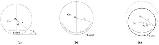
Figure 2.
The existing models for stratified gas–liquid flow: (a): flat interface model; (b): apparent rough surface model; (c): double circle model.
3.2.1. Flat Interface Model
In Figure 2a, the dashed line is the gas–liquid interface. When the gas–liquid interface is flat, the relationship between the central angle, , and the liquid holdup, , can be written as:
3.2.2. Double Circle Model
In Figure 2c, the liquid layer was bounded between the eccentric circle (the center O2) and the pipe wall circle (the center O1). The radiuses of the two circles are R2 and R1, respectively. The point O2 is at a distance above the point O1. There are two extreme cases of the double circle model. When the radius of the eccentric circle R2 is very large, the interface approaches a flat surface, which is similar to the flat interface model. When the radius of the eccentric circle R2 is less than the pipe radius R1, it is a constant thickness liquid film.
As mentioned above, the gas–liquid interface configuration (arc-shaped ADB) is a portion of circle O2, as shown in Figure 3. In order to describe quantitatively the arc-shaped ADB, the location and size of circle O2 must be determined, i.e., the distance, , above the center of the pipe wall and the radius, R2, of the circle O2, or the central angle, and the radius, R2. In the double circle model, the relationship between the liquid holdup, , and the central angles, , and is given as:
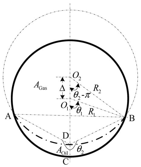
Figure 3.
Geometrical relationship of concave interface.
The relationship between , , R2, and R1 is given by:
According to the definition of the wetted wall fraction, , for a given pipe, if the wetted wall fraction, , is known, the other can be easily calculated. The closure equation is needed for the wetted wall fraction.
The physical mechanism for a liquid film climbing up the pipe wall during stratified flow is still not well understood. This phenomenon is affected by many factors, such as the superficial gas velocity, gas density, and liquid phase surface tension. Under this circumstance, the wetted wall fraction can be calculated by the Fan correlation:
where , are the superficial gas velocity and the critical superficial gas velocity, , respectively. , are the water and liquid surface tension, , respectively. is calculated by the Viles correlation [24]. is the liquid phase Froude number, defined as:
where is the average velocity of the liquid phase.
3.3. Interfacial Friction Factor
The gas–liquid interfacial friction factor is another indispensable closure relationship which is necessary for solving the momentum equations. It is known that the interfacial shear stress greatly affects momentum transfer processes in stratified flow.
3.3.1. Flat Interface Model
In the geometric dimensioning of oil and gas in a circular pipe, the gas–liquid interface shape is assumed to be flat. For laminar flow, the friction factor can be given by the Hagen–Poiseille correlation [25]. For turbulent flow, can be obtained by the Hall correlation [25] and the Chen explicit equation [23]. The friction factor can be calculated in the same way as for , or by the Ouyang–Aziz correlation [26] and Spedding–Hand correlation [27].
The Andritsos–Hanratty correlation [28] is used to obtain the interfacial friction factor :
where .
3.3.2. Double Circle Model
For the double circle model, the friction factor can be obtained by the Ottens correlation [29]. For stratified smooth flow, i.e., , , and for stratified wavy flow, i.e., :
where:
The liquid film velocity at the liquid–gas interface, , is given as:
where the average height of liquid film is given as:
3.4. Slug Liquid Holdup
The liquid holdup of the slug, , can be calculated by the unified mechanistic model [7,21] for any inclination angle. It is derived from the balance between the surface free energy of dispersed bubbles in a slug body and the liquid phase:
where:
The slug liquid holdup should be estimated before solving the combined momentum equitation. It can be given by the Gregory et al. correlation [30]:
The slug length can be estimated as:
4. Results and Discussion
To evaluate the hydrodynamic flat interface model (FIM) and the double interface model (DIM), they were applied to the calculation of liquid holdup and pressure gradient, and compared with the experimental data [21]. Then, the hydrodynamic model was verified with experimental measurements, including of the pressure gradient and liquid holdup. For further verification, the model was compared with that developed by Zhang et al [7].
Table 1 summarizes the experimental conditions. Air, kerosene, and white oil were used in the experiment for the two-phase fluids. The pipes’ inside diameters were 51, 76.3, and 40 mm. The pipe inclination angles varied from 0 to 90 deg. The flow pattern of the experiment was always that of slug flow.

Table 1.
Summary of experimental conditions.
4.1. Comparison of FIM and DIM
Figure 4 shows the comparison for the liquid holdup (an average value of the slug unit), between the two model (i.e., FIM and DIM) predictions and the measured data of the No. 1 experiment. The liquid holdup of slug flow was calculated using the liquid film on the lengths of the slug body and the liquid holdup of the slug body. The predictions of both models and the experimental measurements show good agreement, when the liquid holdup is greater than 0.5, as seen in Figure 4. However, the FIM resulted in greater deviation compared with the experimental data when the liquid holdup decreases to 0.5. In addition, the deviation appears to increase with a decrease in the liquid holdup. The calculations of the DIM are consistently in good accordance with the experiment data.
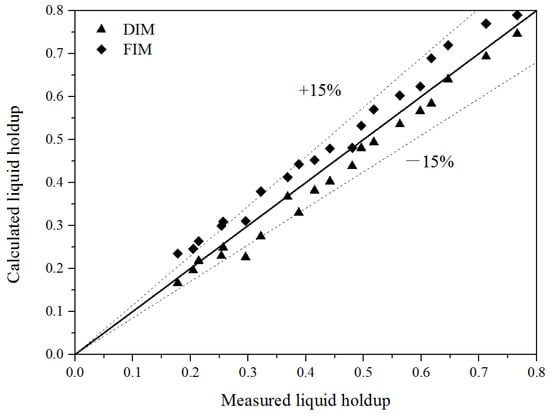
Figure 4.
Comparison of predictions and experiment of liquid holdup for the No. 1 experiment.
In Figure 5, the predictions of pressure gradients for slug flow are compared against the measured data. The pressure gradients calculated in the two models include the shear stress at the pipe wall and the momentum exchange between the liquid film and the slug. As can be noticed, the predictions of the DIM agree with the experimental data better than those of the FIM, and a large number of the predictions of the DIM fall into the ±25% range.
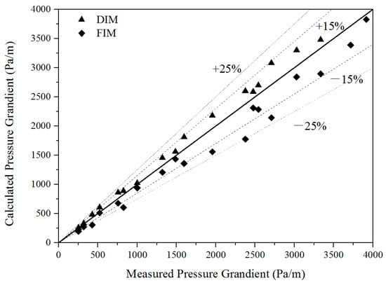
Figure 5.
Comparison between prediction and experiment data of the pressure gradient for the No. 1 experiment.
The liquid holdup prediction of the FIM is greater than that of measurement data. The liquid phase velocity decreases due to the dragging effect, so the liquid holdup must increase. The flat interface of the FIM generates a smaller dragging effect on the liquid phase compared with the curved interface of the DIM.
The pressure gradient of the FIM is underestimated, probably because of the under-prediction of the wetted wall fraction, due to the creep of the liquid film up the pipe wall, which tends to drag more liquid into the slug body. The level of under-prediction is more intensified when the gas superficial velocity is higher, with a constant liquid flow rate. Due to the flat interface along with lower flow resistance, in order to maintain the same flow rates, a smaller pressure gradient is necessary. With decreasing the gas flow rate, the flow resistance decreases, so a smaller pressure gradient is produced. As a result, the differences in the calculated prediction pressure gradient between the two interface assumptions are more uniform.
4.2. Compared with Experiment
The proposed DIM was validated with the measurements of the No. 2 experiment. An experimental study of gas–liquid slug flows with pipe inclinations varying from horizontal to upward vertical was carried out. Figure 6 shows the comparison between predictions of the DIM and the experimental results for liquid holdup. The predictions of liquid holdup are in good agreement with the experimental data, and all the predictions fall into the ±15% range. The calculation gives under-predictions of liquid holdup and the maximum absolute error is 14.8%, which does not exceed 15%.
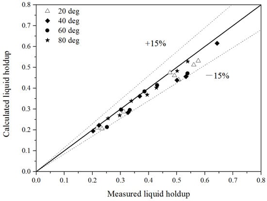
Figure 6.
Comparison of the prediction and experiment for liquid holdup for the No. 2 experiment.
Figure 7 gives the DIM predictions of the pressure gradient compared to the experimental data. The predicted results of the pressure gradient assuming a gas–liquid concave interface exceed the measured data, and fall into the 0–25% range.
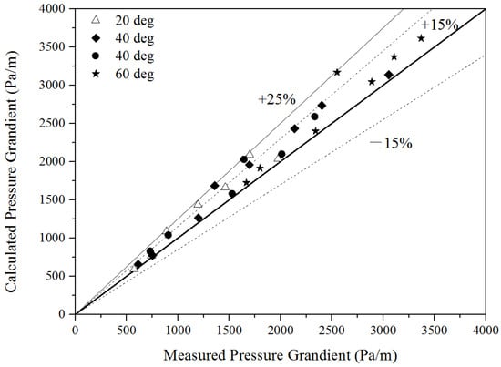
Figure 7.
Comparison of the prediction and experiment for pressure gradient for the No. 2 experiment.
4.3. Comparison with Zhang’s Model
The accuracy of the model was verified by comparing the result of experiment No. 3 [31] with Zhang’s model [7] and the model in this study. The comparison results are shown in Figure 8 and Figure 9, respectively. Table 2 shows the error statistics of the calculation results of the two models. Two kinds of liquid water and white oil were used in the experiment, and air was used as the gas phase medium. The gas apparent velocity is 0.06–20 m/s and the liquid apparent velocity is 0.08–2 m/s.
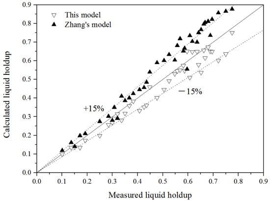
Figure 8.
Comparison of liquid holdup between the two models for the No. 3 experiment.
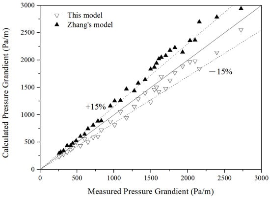
Figure 9.
Comparison of the pressure gradient between the two models for the No. 3 experiment.
Table 2.
Error statistics of the calculation.
The errors in the calculated result using Zhang’s model are relatively large, with an average error of about 15%. In addition, the proportions of errors less than of liquid holdup and the pressure gradient calculated by Zhang’s model are fewer compared to the developed model. The errors in the calculated result of the developed model are evenly distributed, and most of the errors are within the range of 15%. The proportions of errors less than of liquid holdup and the pressure gradient are 72.5% and 82.4% respectively. The average errors of liquid holdup and the pressure gradient are 8.58% and 9.95% respectively. Therefore, the calculation accuracy of the model is high, due to considering the gas–liquid entrainment condition.
5. Conclusions
A hydrodynamic model was developed for gas–liquid two-phase slug flow. The model used the entire liquid film region as the control body, and momentum exchange between the liquid film region and the slug region was introduced into the model. The governing equation can be applied to other flow patterns after deformation, by realizing the unification of various flow patterns.
The gas–liquid entrainment is described in more detail in the model, and entrainment conditions were added into the model. For the important parameters (wall and interfacial friction factors, slug translational velocity, and average slug length), the correlations of these parameters were optimized. Furthermore, the related parameters for the entrainment of liquid droplets and gas bubbles are given in this paper.
Accounting for the gas–liquid interface configuration of the liquid film in the slug body is important; thus, two models (DIM assumed a concave interface, FIM assumed a flat interface) were used for the hydrodynamic predictions. The calculations of pressure gradient and liquid holdup for the DIM were in good accordance with experiment data. For further verification, the calculations of the model were compared with the experimental data and those predicted by Zhang’s model. The errors in the calculated results using the developed model were evenly distributed, and most of the errors were within the range of 15%.
Author Contributions
Methodology, H.L. and J.D.; Formal analysis, H.L. and K.G.; Investigation, J.L. and J.W.; Writing—review & editing, H.Y. and C.L. All authors have read and agreed to the published version of the manuscript.
Funding
This research was funded by the Natural Science Foundation of China (51604282), Natural Science Foundation of Chongqing (cstc2019jcyj-msxmX0268, cstc2019jcyj-msxmX0286 and cstc2019jcyj-msxmX0628).
Informed Consent Statement
Not applicable.
Conflicts of Interest
The authors declare no conflict of interest.
Nomenclature
| Variables | |
| length (m) | |
| R | liquid holdup |
| U | velocity (m/s) |
| A | cross-sectional area inside the pipe (m2) |
| drift velocity (m/s) | |
| empirical coefficient of speed distribution | |
| D | diameter of pipe (m) |
| flow rate (m3/s) | |
| superficial velocity of liquid (m/s) | |
| superficial velocity of gas (m/s) | |
| p | pressure (Pa) |
| g | gravitation (m/s2) |
| S | wetted perimeter (m) |
| f | friction factor |
| Re | Reynolds number |
| Greek letters | |
| inclination angle of pipe | |
| air pocket fraction | |
| shear stress (Pa) | |
| density (kg/m3) | |
| surface tension (N/m) | |
| Subscripts | |
| U | properties at the slug unit |
| S | properties at the liquid slug zone |
| F | properties at the liquid film zone |
| C | properties at the gas pocket |
| i | gas-liquid interface |
References
- Duan, J.-M.; Wang, W.; Zhang, Y.; Liu, H.-S.; Lin, B.-Q.; Gong, J. Calculation on inner wall temperature in oil-gas pipe flow. J. Cent. South Univ. 2012, 19, 1932–1937. [Google Scholar] [CrossRef]
- Guo, W.; Wang, L.; Liu, C. Thermal diffusion response to gas–liquid slug flow and its application in measurement. Int. J. Heat Mass Transf. 2020, 159, 120065. [Google Scholar] [CrossRef]
- Rahimi-Gorji, M.; Van de Sande, L.; Debbaut, C.; Ghorbaniasl, G.; Braet, H.; Cosyns, S.; Remaut, K.; Willaert, W.; Ceelen, W. Intraperitoneal aerosolized drug delivery: Technology, recent developments, and future outlook. Adv. Drug Deliv. Rev. 2020, 160, 105–114. [Google Scholar] [CrossRef]
- Van de Sande, L.; Rahimi-Gorji, M.; Giordano, S.; Davoli, E.; Matteo, C.; Detlefsen, S.; D’Herde, K.; Braet, H.; Shariati, M.; Remaut, K.; et al. Electrostatic Intraperitoneal Aerosol Delivery of Nanoparticles: Proof of Concept and Preclinical Validation. Adv. Healthc. Mater. 2020, 9, 2000655. [Google Scholar] [CrossRef]
- Sarica, C.; Panacharoensawad, E. Review of Paraffin Deposition Research under Multiphase Flow Conditions. Energy Fuels 2012, 26, 3968–3978. [Google Scholar] [CrossRef]
- Zhai, L.; Xia, H.; Xie, H.; Yang, J. Structure Detection of Horizontal Gas–Liquid Slug Flow Using Ultrasonic Transducer and Conductance Sensor. IEEE Trans. Instrum. Meas. 2021, 70, 1–10. [Google Scholar] [CrossRef]
- Zhang, H.-Q.; Wang, Q.; Sarica, C.; Brill, J.P. Unified Model for Gas-Liquid Pipe Flow via Slug Dynamics—Part 1: Model Development. J. Energy Resour. Technol. 2003, 125, 266–273. [Google Scholar] [CrossRef]
- Zhai, L.; Wu, Y.; Yang, J.; Xie, H. Reconstruction of Taylor Bubbles in Slug Flow Using a Direct-Image Multielectrode Conductance Sensor. IEEE Sens. J. 2020, 20, 10643–10652. [Google Scholar] [CrossRef]
- Mei, M.; Felis, F.; Hébrard, G.; Dietrich, N.; Loubière, K. Hydrodynamics of Gas–Liquid Slug Flows in a Long In-Plane Spiral Shaped Milli-Reactor. Theor. Found. Chem. Eng. 2020, 54, 25–47. [Google Scholar] [CrossRef]
- Liu, G.; Hao, Z.; Wang, Y.; Ren, W. Research on the Dynamic Responses of Simply Supported Horizontal Pipes Conveying Gas-Liquid Two-Phase Slug Flow. Processes 2021, 9, 83. [Google Scholar] [CrossRef]
- Taitel, Y.; Dukler, A.E. A model for predicting flow regime transitions in horizontal and near horizontal gas-liquid flow. AIChE J. 1976, 22, 47–55. [Google Scholar] [CrossRef]
- Barnea, D. A unified model for predicting flow-pattern transitions for the whole range of pipe inclinations. Int. J. Multiph. Flow 1987, 13, 1–12. [Google Scholar] [CrossRef]
- Kokal, S.L.; Stanislav, J.F. An experimental study of two-phase flow in slightly inclined pipes—I. Flow patterns. Chem. Eng. Sci. 1989, 44, 665–679. [Google Scholar] [CrossRef]
- Spedding, P.L.; Spence, D.R.; Hands, N.P. Prediction of holdup in two-phase gas-liquid inclined flow. Chem. Eng. J. 1990, 45, 55–74. [Google Scholar] [CrossRef]
- Bendiksen, K.H.; Maines, D.; Moe, R.; Nuland, S. The Dynamic Two-Fluid Model OLGA: Theory and Application. SPE Prod. Eng. 1991, 6, 171–180. [Google Scholar] [CrossRef]
- Henau, V.D.; Raithby, G.D. A transient two-fluid model for the simulation of slug flow in pipelines—I. Theory. Int. J. Multiph. Flow 1995, 21, 335–349. [Google Scholar] [CrossRef]
- De Henau, V.; Raithby, G.D. A transient two-fluid model for the simulation of slug flow in pipelines—II. Validation. Int. J. Multiph. Flow 1995, 21, 335–349. [Google Scholar] [CrossRef]
- Issa, R.I.; Kempf, M.H.W. Simulation of slug flow in horizontal and nearly horizontal pipes with the two-fluid model. Int. J. Multiph. Flow 2003, 29, 69–95. [Google Scholar] [CrossRef]
- Losi, G.; Arnone, D.; Correra, S.; Poesio, P. Modelling and statistical analysis of high viscosity oil/air slug flow characteristics in a small diameter horizontal pipe. Chem. Eng. Sci. 2016, 148, 190–202. [Google Scholar] [CrossRef]
- Arabi, A.; Salhi, Y.; Zenati, Y.; Si-Ahmed, E.; Legrand, J. On gas-liquid intermittent flow in a horizontal pipe: Influence of sub-regime on slug frequency. Chem. Eng. Sci. 2020, 211, 115251. [Google Scholar] [CrossRef]
- Zhang, H.-Q.; Wang, Q.; Sarica, C.; Brill, J.P. Unified Model for Gas-Liquid Pipe Flow via Slug Dynamics—Part 2: Model Validation. J. Energy Resour. Technol. 2003, 125, 274–283. [Google Scholar] [CrossRef]
- Grolman, E.; Fortuin, J.M.H. Gas-liquid flow in slightly inclined pipes. Chem. Eng. Sci. 1997, 52, 4461–4471. [Google Scholar] [CrossRef]
- Chen, N.H. An Explicit Equation for Friction Factor in Pipe. Ind. Eng. Chem. Fundam. 1979, 18, 296–297. [Google Scholar] [CrossRef]
- Viles, J.C. Predicting Liquid Re-Entrainment in Horizontal Separators. J. Pet. Technol. 2013, 45, 405–409. [Google Scholar] [CrossRef]
- Taitel, Y.; Shoham, O.; Brill, J. Simplified transient solution and simulation of two-phase flow in pipelines. Chem. Eng. Sci. 1989, 44, 1353–1359. [Google Scholar] [CrossRef]
- Ouyang, L.B.; Aziz, K. Development of New Wall Friction Factor and Interfacial Friction Factor Correlations for Gas-Liquid Stratified Flow in Wells and Pipelines. In Proceedings of the SPE Western Regional Meeting, Anchorage, AK, USA, 22–24 May 1996. [Google Scholar]
- Spedding, P.L.; Hand, N.P. Prediction in stratified gas-liquid co-current flow in horizontal pipelines. Int. J. Heat Mass Transf. 1997, 40, 1923–1935. [Google Scholar] [CrossRef]
- Andritsos, N.; Hanratty, T.J. Influence of interfacial waves in stratified gas—Liquid flows. AIChE J. 1987, 33, 444–454. [Google Scholar] [CrossRef]
- Ottens, M.; Hoefsloot, H.C.J.; Hamersma, P.J. Correlations Predicting Liquid Hold-up and Pressure Gradient in Steady-State (Nearly) Horizontal Co-Current Gas-Liquid Pipe Flow. Chem. Eng. Res. Des. 2001, 79, 581–592. [Google Scholar] [CrossRef]
- Gregory, G.A.; Nicholson, M.K.; Aziz, K. Correlation of the liquid volume fraction in the slug for horizontal gas-liquid slug flow. Int. J. Multiph. Flow 1978, 4, 33–39. [Google Scholar] [CrossRef]
- Wang, H.; Li, Y.; Cai, X.; Song, C.; Meng, L. Development and verification of unified model based on slug flow for gas-liquid two-phase flow. CIESC J. 2013, 64, 3549–3557. [Google Scholar]
Publisher’s Note: MDPI stays neutral with regard to jurisdictional claims in published maps and institutional affiliations. |
© 2022 by the authors. Licensee MDPI, Basel, Switzerland. This article is an open access article distributed under the terms and conditions of the Creative Commons Attribution (CC BY) license (https://creativecommons.org/licenses/by/4.0/).