Synthesizing Nuclear Magnetic Resonance (NMR) Outputs for Clastic Rocks Using Machine Learning Methods, Examples from North West Shelf and Perth Basin, Western Australia

Abstract

A nuclear magnetic resonance (NMR) logging tool can provide important rock and fluid properties that are necessary for a reliable reservoir evaluation. Pore size distribution based on T₂ relaxation time and resulting permeability are among those parameters that cannot be provided by conventional logging tools. For wells drilled before the 1990s and for many recent wells there is no NMR data available due to the tool availability and the logging cost, respectively. This study used a large database of combinable magnetic resonance (CMR) to assess the performance of several well-known machine learning (ML) methods to generate some of the NMR tool’s outputs for clastic rocks using typical well-logs as inputs. NMR tool’s outputs, such as clay bound water (CBW), irreducible pore fluid (known as bulk volume irreducible, BVI), producible fluid (known as the free fluid index, FFI), logarithmic mean of T₂ relaxation time (T_2LM), irreducible water saturation (S_wirr), and permeability from Coates and SDR models were generated in this study. The well logs were collected from 14 wells of Western Australia (WA) within 3 offshore basins. About 80% of the data points were used for training and validation purposes and 20% of the whole data was kept as a blind set with no involvement in the training process to check the validity of the ML methods. The comparison of results shows that the Adaptive Boosting, known as AdaBoost model, has given the most impressive performance to predict CBW, FFI, permeability, T_2LM, and S_Wirr for the blind set with R2 more than 0.9. The accuracy of the ML model for the blind dataset suggests that the approach can be used to generate NMR tool outputs with high accuracy.

1. Introduction

Well logging tools provide continuous series of subsurface information that can characterize the rock and fluid properties. The nuclear magnetic resonance (NMR) logging tool can provide some additional important information that makes it a very useful tool in many disciplines, such as oil and gas, groundwater, carbon capture and storage (CCS), and natural gas and hydrogen storage that deal with subsurface rock characterization. NMR is a phenomenon that describes the response of hydrogen to a magnetic field [1]. The relaxation of hydrogen protons and their quantification is the central basis of the NMR technique. The petrophysical evaluation of rocks from the NMR log is a well-established practice in the petroleum industry. The NMR data can provide several rock properties such as porosity, pore size distribution, permeability [2,3,4,5,6,7,8,9,10]. In saturated porous media, the NMR T₂ relaxation rate is a function of individual intrinsic (or bulk), surface, and diffusion relaxation processes governed by the following equation [11]:

$$\frac{1}{T_2}=\frac{1}{T_{2bulk}}+\frac{1}{T_{2surface}}+\frac{1}{T_{2diffusion}}$$

(1)

Protons associated with clay-bound water (CBW) and fluid in small pores display short T₂, whereas fluid in larger pores shows longer T₂ relaxation times. Generally, a T₂ cutoff can be designated to distinguish between CBW, irreducible pore fluids or pores containing bound water (known as bulk volume irreducible, BVI), and producible fluids (known as the free fluid index, FFI) [1,5,12]. The T₂ cutoff can be determined experimentally from the comparison of NMR curves obtained for core samples at different saturation levels or assumed based on lithology [12,13,14]. Generally, the T₂ distribution is represented by a set of 8 bins porosities (BP1 to BP8) determined for a set of T₂ cutoffs. For clastic rocks, the cutoffs shown in Figure 1 are generally used to determine the bin porosities and therefore different types of pore systems as below:

$$CBW= {\displaystyle \sum }_{i =1}^{2}BPi$$

(2)

$$BVI= {\displaystyle \sum }_{i=3}^{4}BPi$$

(3)

$$FFI= {\displaystyle \sum }_{i=5}^{8}BPi$$

(4)

$${\varnothing }_e= {\displaystyle \sum }_{i=3}^{8}BPi= BVI+FFI$$

(5)

$${\varnothing }_t= {\displaystyle \sum }_{i=1}^{8}BPi= CBW+BVI+FFI$$

(6)

$$S_{wirr}= \frac{BVI}{BVI+FFI}= \frac{BVI}{{\varnothing }_e}$$

(7)

where BP = bin porosity; CBW = clay bound water; BVI = bulk volume irreducible; FFI = free fluid index; ∅e = effective porosity; ∅t = total porosity; and S_wirr = irreducible water saturation.

There are several models to estimate permeability based on NMR T₂ relaxation data, from which the Coates and the SDR (Schlumberger-Doll-Research) models are the most widely used [8,13,14,15]. In the Coates model, permeability estimation depends on the T₂ cutoff value that separates FFI from BVI:

$$k={\left[(\frac{{\varnothing }_e}{\mathrm{C}}{)}^2(\frac{\mathrm{FFI}}{\mathrm{BVI}})\right]}^2$$

(8)

where k is the matrix permeability (mD), ${\varnothing }_e$ is the NMR effective porosity (%), and C is a constant specific to the formation that reflects the correlation between the rock’s pore throat and pore size, and in fact, it is a function of pore geometry and is generally considered 10 as a default value for clastic rocks. FFI = the free fluid index, and BVI = the bound volume of irreducible water.

In the SDR model, permeability is determined using the logarithmic mean of the T₂ distribution:

$$k=a{T}_{2LM}^2{\varnothing }_e{}^4$$

(9)

where T_2LM is the logarithmic mean of the T₂ distribution, milliseconds; and “a” is a coefficient that depends on formation type and has to be determined through calibration with core porosity. “a” is generally close to 4 for sandstone.

2. Data Acquisition and Preparation

In this study, a large dataset from WA offshore basins was used to evaluate the performance of several ML methods to synthesize NMR logging tool outputs. A total of available 16,025 data points from 16 formations (Figure 2) with the age range of Permian to Tertiary were used. The data were collected from 14 wells with a complete set of CMR and conventional logs, such as Scarborough and Pluto wells. Wells are located within 3 main offshore basins of WA (Browse, Northern Carnarvon, and Perth Basins) with a depth range of from 1188 to 4138 meters (

Table 1. The list of the basins, formations, and their details used for this study.

Basin	Formation	Age	Depth (m)	Fluid Type	Main Lithology
Browse	Bassett	Tertiary	1390–1408	Gas-Cond.	Sandstone
Browse	Grebe	Tertiary	1312–1385	Gas-Cond.	Sandstone
Browse	Nome	Triassic	3823–3848	Gas	Sandstone
Browse	Plover	Jurassic	3776–3823	Gas	Sandstone
Browse	Vulcan	Juras. to Cre.	3942–4138	Oil	Sandstone
N. Carnarvon	Angel	Jurassic	3400–3700	Oil	Sandstone
N. Carnarvon	Barrow Group	Cretacous	1890–1936	Oil	Sandstone
N. Carnarvon	Brigadier	Triassic	3037–3162	Oil	Sandstone
N. Carnarvon	Forestier	Cretacous	2983–3147	Brine	Claystone
N. Carnarvon	Muderong	Cretacous	2960–2982	Brine	Shale
N. Carnarvon	Mungaroo	Triassic	3045–3710	Oil and Gas	Sandstone
Perth	Cattamarra	Jurassic	2940–3052	Oil	Sandstone
Perth	Dongara	Triassic	1276–1281	Oil	Sandstone
Perth	High Cliff	Permian	1310–1476	Oil	Sandstone
Perth	IRCM	Permian	1278–1475	Oil	Sandstone
Perth	Kockatea	Triassic	1188–1427	Brine	Shale

). All data were combined in one file and after randomizing, 80% of data (12,820 data points) were used for training purposes and 20% (3205 data points) as blind samples to check the ML performance.

Although some typical well logs have a weak correlation with NMR log outputs they were not excluded since it was realized that even removing those with the smallest prediction contribution reduces the ML performance. The well logs used in this study as ML’s inputs are density (RHOB), neutron (NPHI), photoelectric (PEF), resistivity (deep, shallow, and very shallow), and sonic (DT). Additional inputs such as volume of shale (Vsh) from GR and effective porosity calculated from density tool (PHIDeffe) were included to improve model accuracy to synthesize NMR log outputs. Coates permeability (kCoates), SDR permeability (kSDR), FFI, BVI, S_wirr, and T_2LM are ML’s outputs.

Assuming a linear relationship, the volume of shale was calculated for all formations with the following equation:

$$Vsh=\frac{G{R}_{\log }-G{R}_{\min }}{G{R}_{\max }-G{R}_{\min }}$$

(10)

This is also known as the GR index equation (I_GR). The GR_min and GR_max values are the values of the sand and shale lines respectively taken from the GR reading for each well.

The effective porosity in shaly formations may be calculated by including a correction for the contribution of shale to the log measurements. Density log was used to calculate effective porosity for shaly formations using the following equation:

$${\varphi }_{Dshc}\approx {\varphi }_e=\frac{{\rho }_{ma}-{\rho }_b}{{\rho }_{ma}-{\rho }_f}-V_{sh}\frac{{\rho }_{ma}-{\rho }_{sh}}{{\rho }_{ma}-{\rho }_f}$$

(11)

where ρ_b = bulk density (g/cc); ρ_f = fluid density (g/cc); ρ_ma = matrix density (g/cc); V_sh = volumetric fraction of shale; ρ_sh = shale bulk density (g/cc) that was identified for each well separately; ϕ_Dshc = shale corrected density porosity and ϕ_e = effective porosity.

Synthesizing NMR log outputs heavily relies upon the quality and consistency of the input dataset available to build the ML model. Log data require proper quality control and editing task to make them reliable as input parameters. The most common errors observed in well logs are depth mismatching (depth differences between different logs); bad hole data that can be detected on caliper and DHRO logs; cycle skipping where occasionally tools, such as the sonic log miss out a reading due to a weak signal, leading to sudden blips on the well log; and spikes that are the unusual response of logs due to tool failure. All well logs were quality controlled and checked for the above-mentioned errors. A careful depth match was conducted between NMR and other logs using GR that was available for both datasets.

3. Machine Learning (ML) Models

Machine learning (ML) is a computer program that can be trained to perform assigned tasks or make decisions [16,17]. ML methods enable computer systems to learn patterns from data observations [18,19,20]. Training is the process of learning from data during which the model is exposed to a proportion (usually 70–85%) of the data known as the training set. Training is accomplished by optimizing the model’s hyperparameters to best match the training set. To improve the generalizability of the trained model, a specified fraction (usually 15–30%) of the data are used to test and validate the performance of the trained model. To evaluate the overall performance of the model, it is good practice to also blind-test it on a held-out portion of the data [21]. Some related examples of the application of ML are synthetic well log generation [22,23,24,25]; porosity, permeability, and other petrophysical parameters prediction [23,26,27,28,29,30,31,32,33,34]; permeability predictions [35,36,37,38,39,40,41,42,43]; and geomechanical property estimation [44,45].

Different ML methods have been used to synthesize the NMR logs [24,25,46], but it is critical to find the best approach that provides the most accurate prediction. Ensemble learning improves machine learning outputs by combining several models. Ensemble learning provides better predictive performance compared to a single model. The two most widely used ensemble methods are bagging and boosting models. Bagging uses a training set of individual models in which random subsets drawn by bootstrap sampling with replacement from the training data are used to build multiple decision trees in a parallel way. Each model is trained by a random subset of the data and the overall performance is obtained as the majority vote of the performances of the individual models [47,48]. Random forest is a good example of this type of ensemble learning [49]. Boosting, on the other hand, is a sequential type of ensemble learning that utilises weighted random subsets of the training data to build separate decision trees which are then combined through a weighted majority vote [47,48]. The weighting assigned to each subset of data learns from mistakes made by the previous model and adjusts over time by its contribution to the overall performance [48]. Adaptive Boosting (AdaBoost) is an example of boosting ensemble learning.

The most common models, which can easily be applied in most statistical packages, have been used for this study using Python. A total of five machine learning methods including artificial neural network (ANN), k-nearest neighbor (kNN), support vector machine (SVM), Adaptive Boosting (AdaBoost), and random forest (RF) were utilized to assess the performance of each for prediction of NMR log outputs. A very brief explanation of the methods used in the paper is given below:

Application of artificial neural networks (ANN) in the industry has proved to be a valuable tool for rock and fluid property prediction (e.g., [23,30,50,51]). A neural network is a mathematical model that can be trained to solve a problem. ANN can distinguish complex patterns within a dataset that making it possible to get the existing nonlinear relationships that are normally not well understood between input and output parameters. The basic structure of an ANN is neurons and their connection strengths (weight). Neural networks are classified by the way they are trained, using either supervised or unsupervised learning. In supervised learning, the ANN will be trained using a dataset for which both the input and output values are available to the program. In unsupervised learning, the ANN is presented with a series of inputs and lets the neural network look for patterns itself. In a classic neural data processing system, the database is divided into training and test sets. The training set is used to develop the desired network that is used to help the network adjust the weights between its neurons (supervised training). In this study, a three-layered back propagation supervised neural network was trained using the rectified linear unit function as the activation function for the hidden layer and L-BFGS-B (an optimization algorithm in the family of quasi-Newton methods) for the solver for weight optimization with 200 neurons in hidden layers.

K-nearest neighbor (kNN) is a simple supervised machine learning method used in classification and regression cases. This algorithm calculates the distances between an unclassified case and the nearest k training cases. The kNN algorithm uses the k nearest points of the input to predict the response [52]. Indeed, the method searches for k closest training examples in feature space and uses their average as a prediction. A variety of distance metrics can be used, however, the most commonly used is the Euclidean distance [53]. In this study, Euclidean metric with uniform weight and five neighbors were used.

Support vector machine (SVM) is a supervised machine learning technique that supports both classification and regression problems. SVM separates the attribute space with a hyperplane, thus maximizing the margin between the instances of different classes or class values. SVM performs linear regression in a high dimensional feature space and its performance depends on a good setting of cost (penalty term for loss and applies for classification and regression tasks, C), regression loss epsilon (defines the distance from true values within which no penalty is associated with predicted values, ε) and kernel parameters. The Kernel is a function that transforms attribute space to a new feature space to fit the maximum-margin hyperplane, thus allowing the algorithm to create the model with linear, polynomial, radial basis function (RBF) and Sigmoid kernels. In this study, radial basis function (RBF) was used as the kernel function, the C was set to 1.0, and regression loss epsilon was set to 0.1.

The AdaBoost algorithm, presented by Freund and Schapire [54] is a boosting ensemble model and works especially well with the decision tree. AdaBoost is fast, simple, and easy to program with no critical parameters to tune (except for the number of estimators) [55]. AdaBoost trains the base classifiers using random bootstraps data samples selected from original data and then integrate their decisions through a weighted majority vote. Firstly, it allocates equal weights to all the training data and then adjustments of weights are made based on the misclassifications obtained through the initial base classifier. For the next modified training dataset, the weights of misclassified data are increased to increase the chances of occurrence of misclassified samples in the next training dataset [56]. The AdaBoost algorithm has an accuracy-oriented tactic and concentrates on the incorrectly classified samples while increasing the weight until it approaches the target.

Random forest (RF) is an ensemble learning technique that can be used for classification and regression tasks. Random forest is an ensemble model using bagging as the ensemble method and decision tree as the individual model that builds a large number of decision trees from bootstrap samples of the training data [49]. When developing individual trees, a random subset of attributes is drawn from which the best attribute for the split is selected. The final model is based on the majority vote from individually developed trees in the forest. RF does not require extensive tuning for its parameters that are the number of trees and growth control. In this study, 10 decision trees were included in the forest.

4. Results

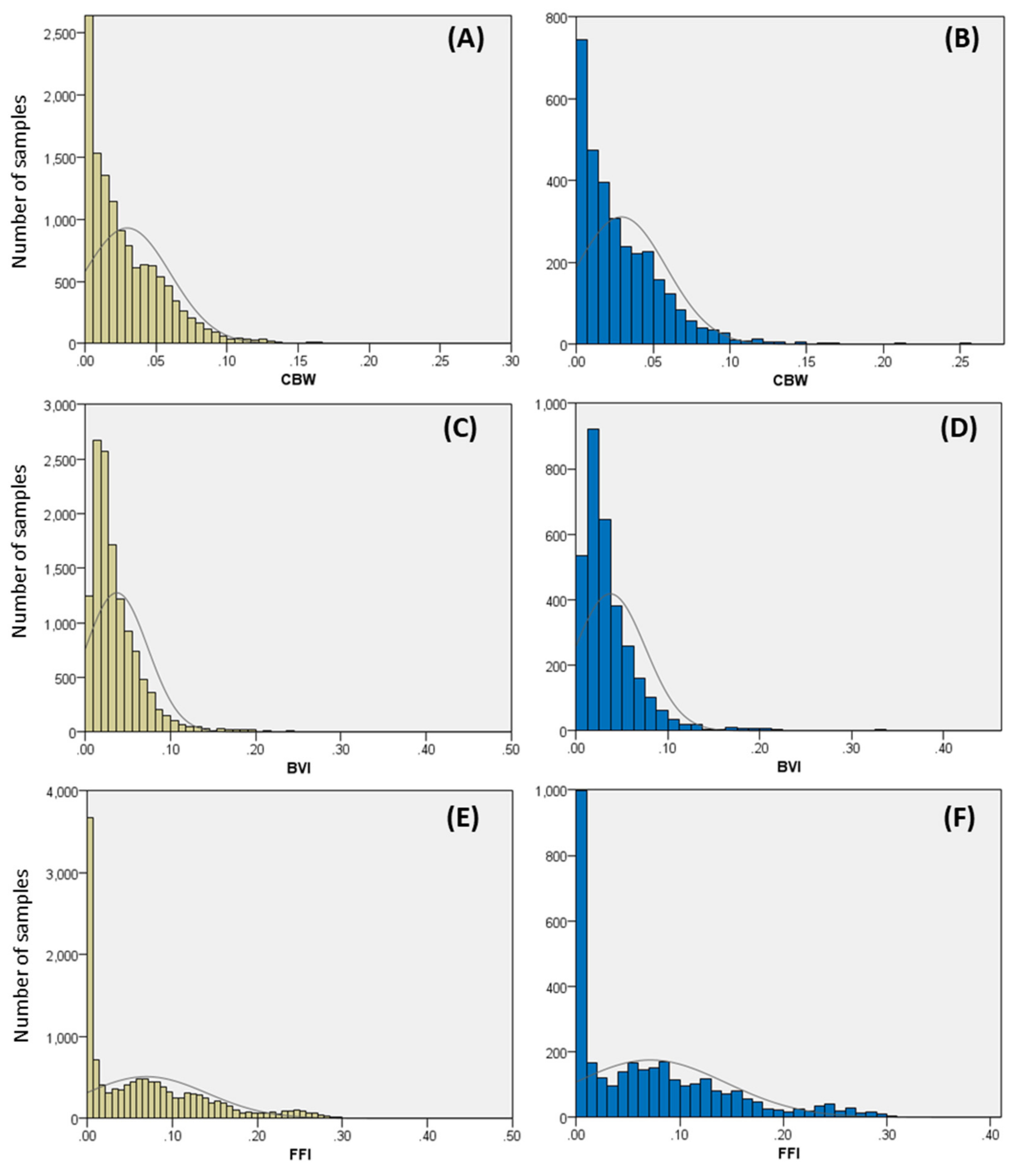
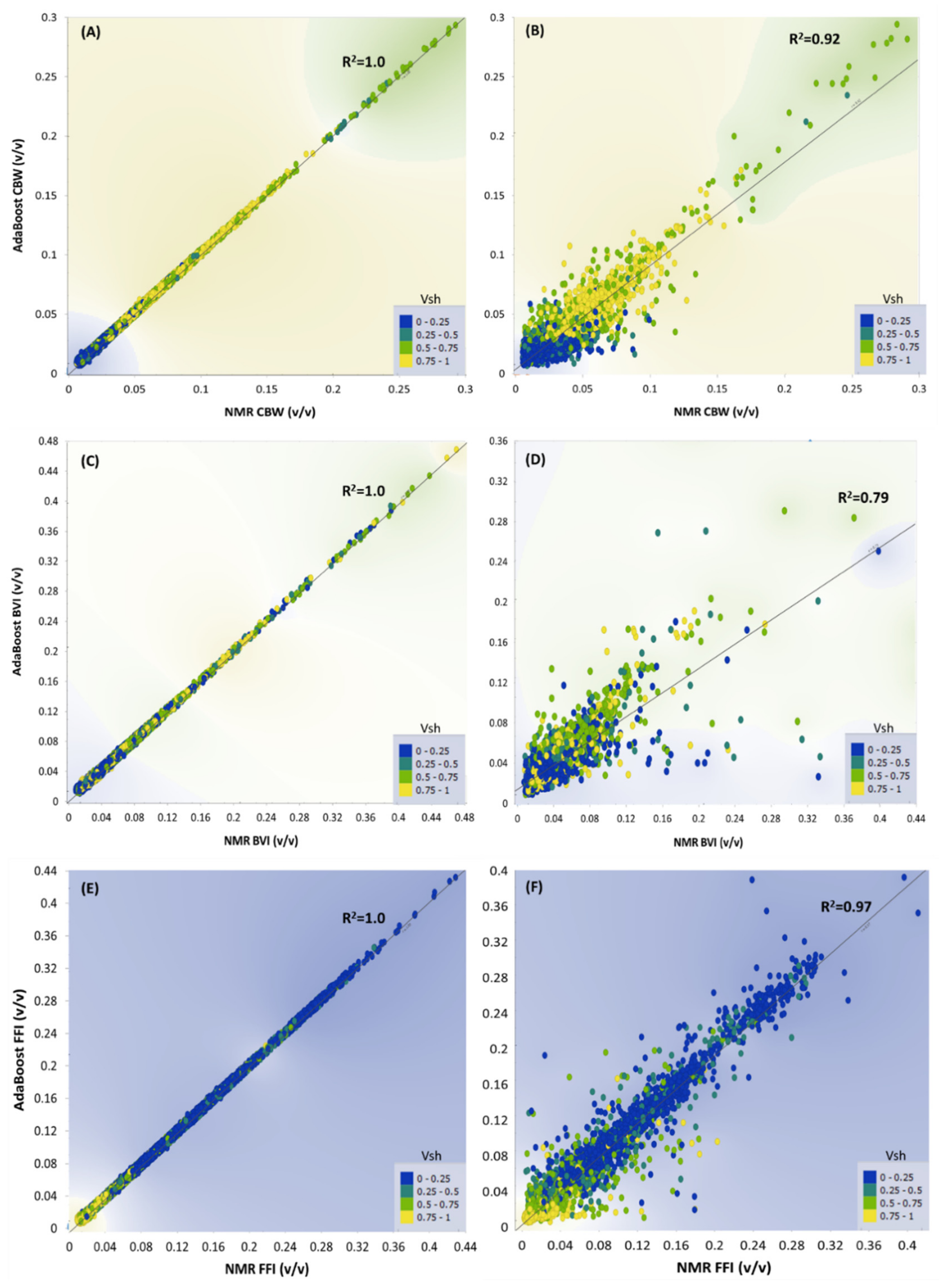
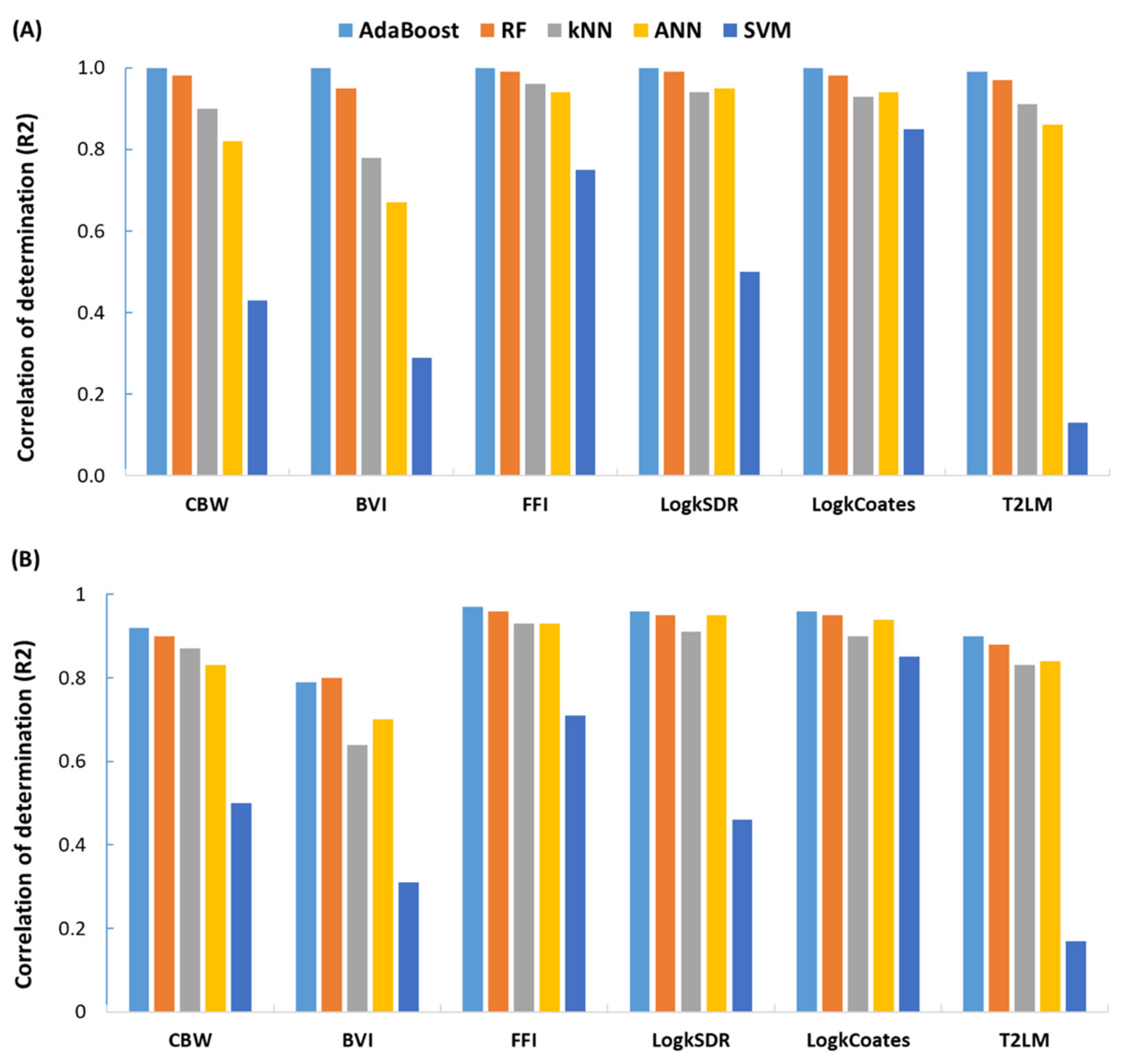
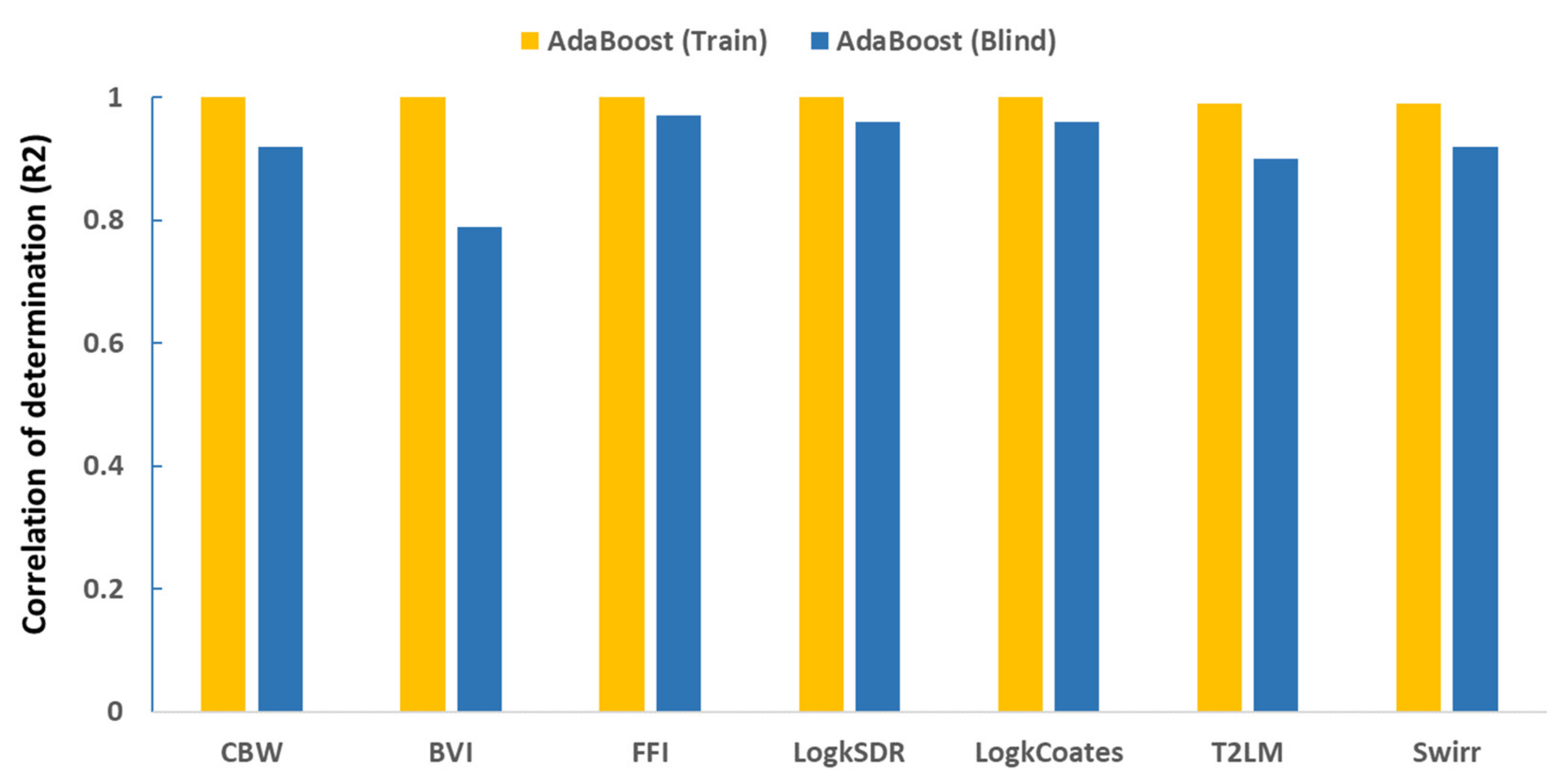
4.1. Porosity Prediction

NMR log provides rock’s pore volumes based on the hydrogen content. Ignoring structural hydrogen, hydrogen within the chemical structure of minerals such as clays and gypsum, it generally exists in pore-filling fluids, such as water and hydrocarbons. Based on the NMR T₂ cutoffs, three types of pore spaces can be detected by the NMR tool including CBW, BVI, and FFI. Clay bond water (CBW) is a layer(s) of water molecules that cover the surface of clay minerals, therefore, occupy part of the pore spaces. Clay particles generally have a negative charge at the surface. The accumulation of negative charges attracts cations and water molecules on the surface of clay particles known as CBW. CBW is strongly attached to the surface of clays and shows a low T₂. In clastic rocks, pore spaces that occur between T₂ values of 0.3 to 3.0 ms are considered CBW. Other studies by [57,58] indicates different cutoff values for shale reservoirs. The volume of CBW depends mostly on the type of clay, and pore water salinity. In well log interpretation, effective porosity is defined as total porosity minus CBW and there are different approaches to quantify CBW volume using Vsh. Figure 3A,B show CBW variations in the training and blind datasets. Adaboost both in training and blind datasets shows the best performance to predict CBW (Figure 4A,B) followed by RF, kNN, and ANN. Based on Pearson correlation the most influencing inputs to predict CBW in the order of importance are NPHI, Vsh, and DT. A confidence interval of 95% was used for the presentation of all results in this study.

BVI or bulk volume irreducible represents pore fluids or pores containing bound water or immobile water. Pore spaces associated with BVI are small pores with high capillary pressure where hydrocarbon buoyance pressure is unable to displace the pore filling water. In clastic rocks, pore spaces that occur between T₂ values of 3.0 to 33.0 ms are considered BVI. Figure 3C,D show BVI variations in the training and blind datasets. Based on Pearson correlation the most influencing inputs to predict BVI in the order of importance are DT, PEF, and RHOB. Adaboost both in training and blind datasets shows the best performance to predict BVI (Figure 4C,D) followed by RF, kNN, and ANN.

FFI or free fluid index indicates the relatively larger pore spaces where mobile or producible fluids reside. In clastic rocks pore spaces with T₂ values larger than 33.0 ms are considered FFI. Figure 3E,F show FFI variations in the training and blind datasets. The same as CBW and BWI, Adaboost predicts FFI with high performance both in training and blind datasets (Figure 4E,F) followed by RF, ANN, and kNN. The most influencing inputs to predict FFI in the order of importance are PHIDEFFE, RHOB, and Vsh.

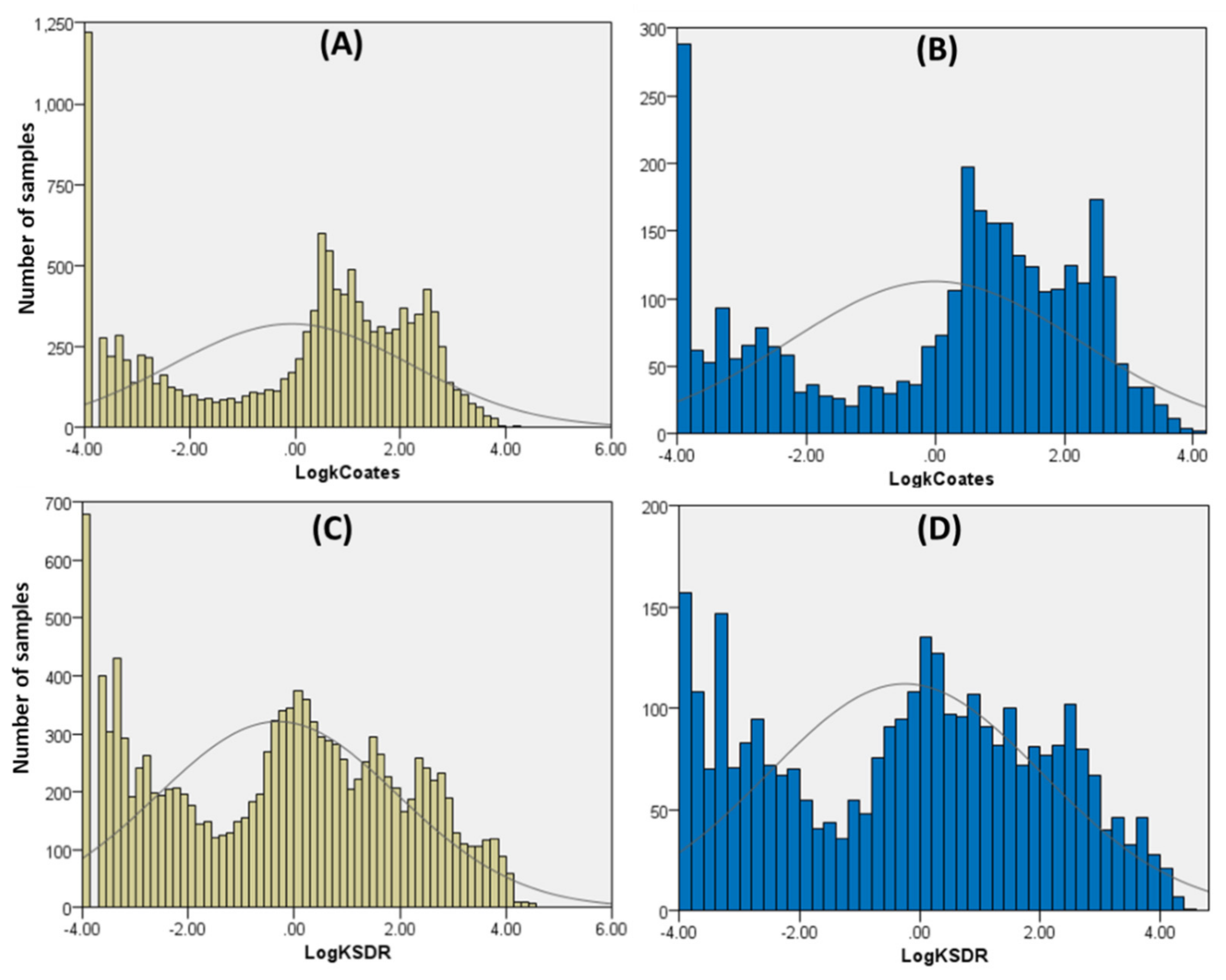
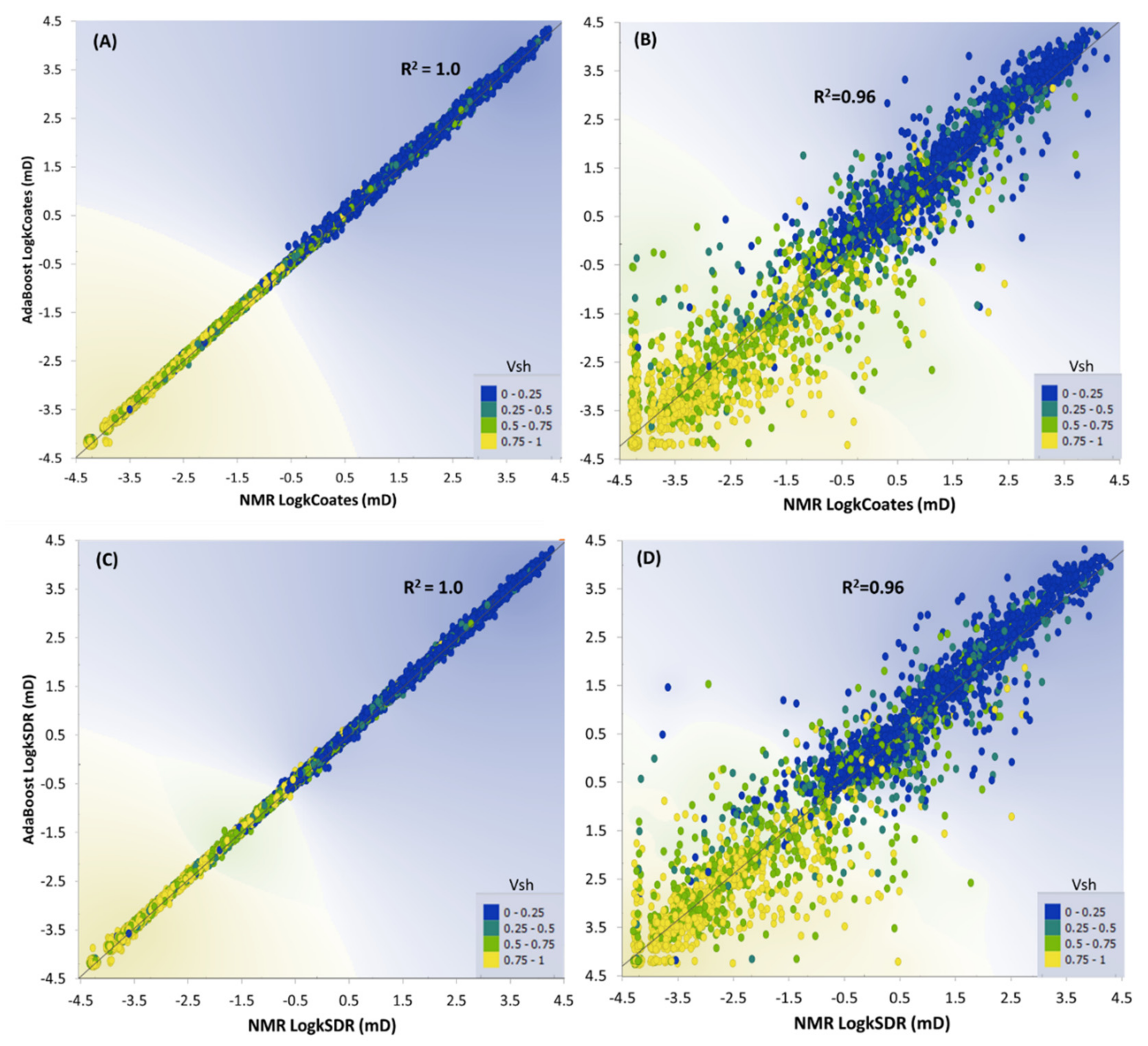
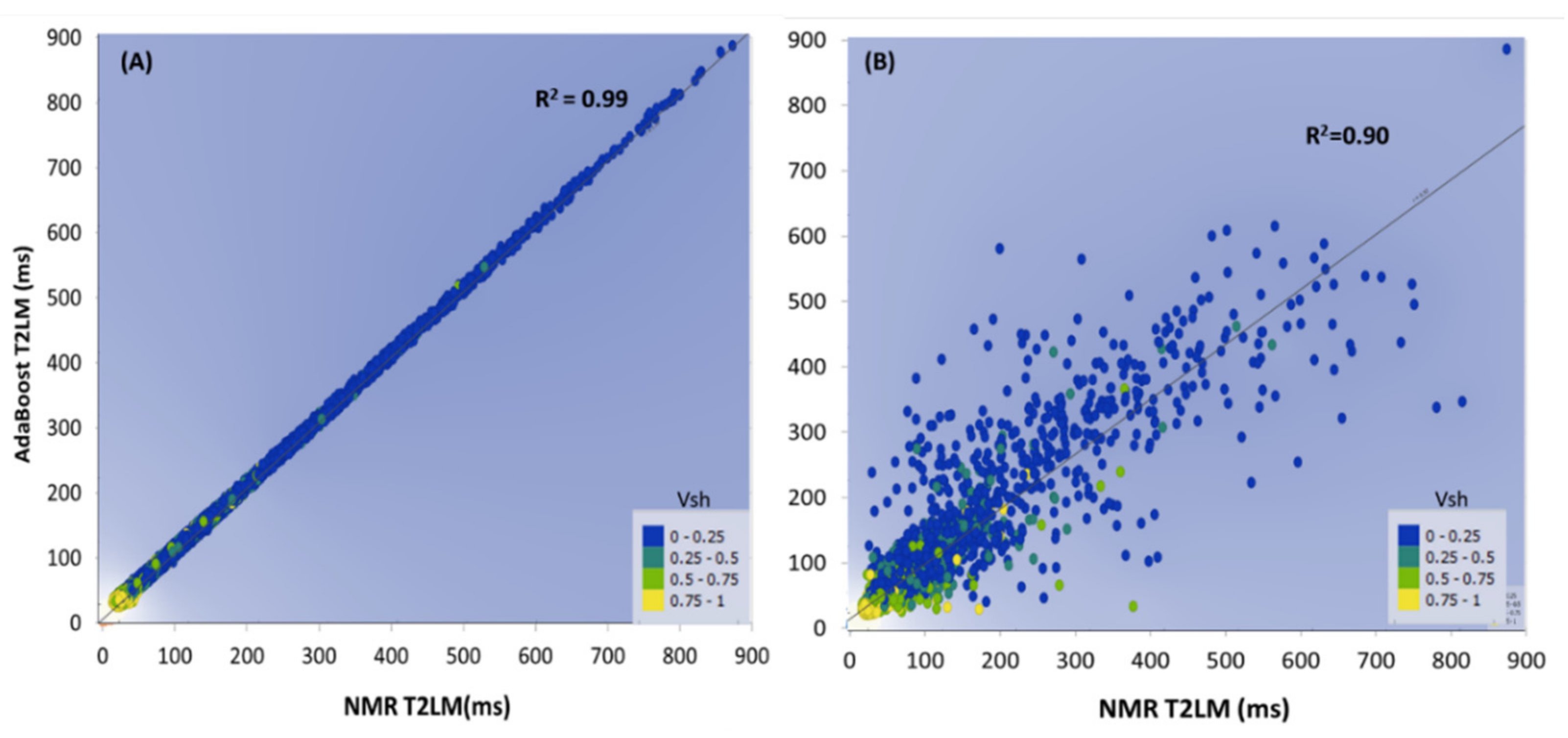
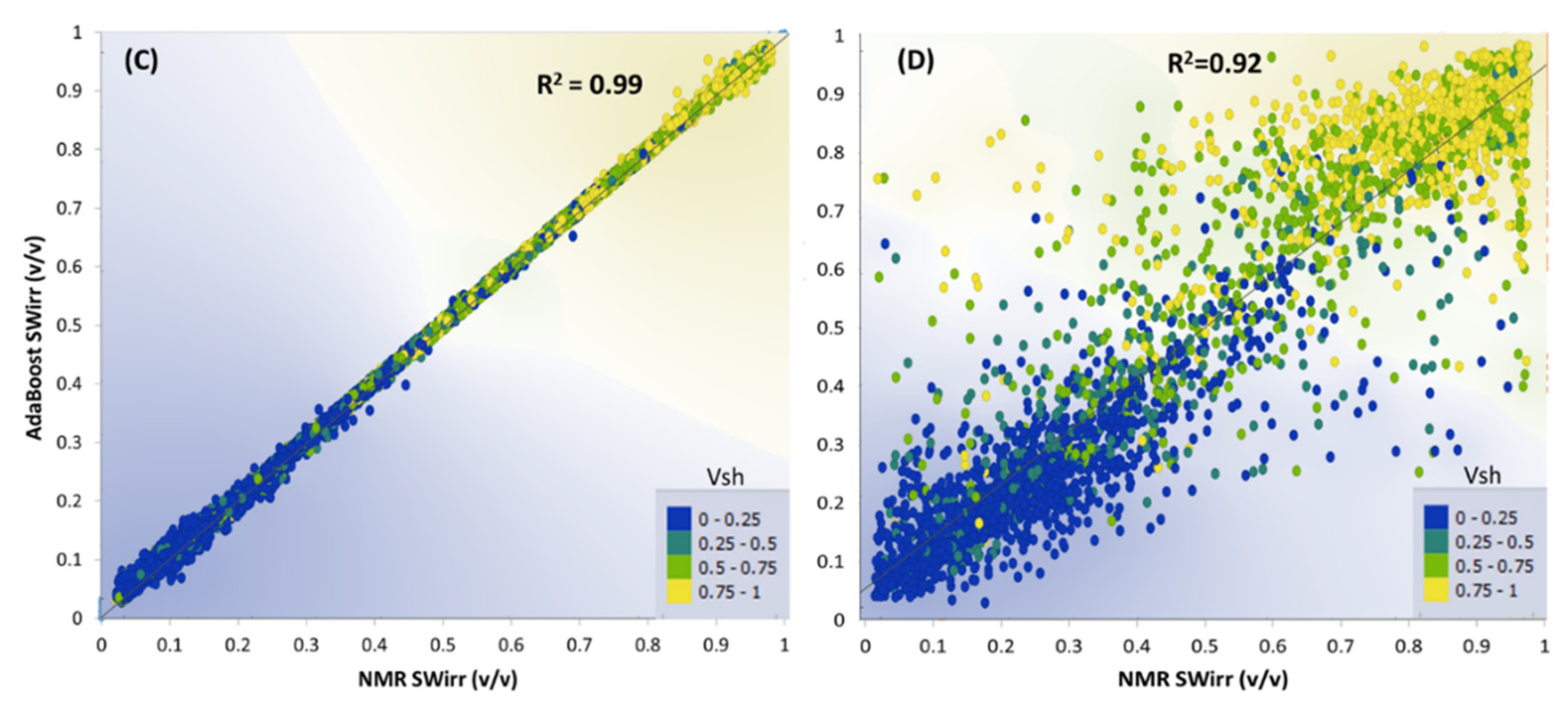
4.2. Permeability Prediction

In this study, Coates and SDR permeabilities were predicted using different ML models. The logarithm of permeability as output proved to increase the ML models’ performance to predict permeability. Figure 5 shows Coates and SDR permeabilities variations in the training and blind datasets. Adaboost both in training and blind datasets shows the best performance to predict permeability values (Figure 6) followed by RF, ANN, and kNN. Based on Pearson correlation the most influencing inputs to predict permeability in the order of importance are PHIDEFFE, Vsh, and RHOB.

T_2LM and S_Wirr were also generated separately. The same as other outputs, Adaboost performed better in both training and blind datasets to predict these parameters (Figure 7). PHIDEFFE, RHOB, and Vsh were the most influential inputs for T_2LM and S_wirr prediction.

Figure 8 compares the performance of each ML method in the prediction of the NMR tool’s outputs for the Training and Blind datasets. The R2 coefficient was used to measure the prediction accuracy of the model.

5. Discussion and Conclusions

In this study NMR tool’s outputs were synthesized from conventional well logs using 5 ML techniques. The AdaBoost model shows the best performance to predict CBW, FFI, permeability, T_2LM, and S_Wirr for the blind set with R2 of more than 0.9 (Figure 9). BVI was the only parameter that was predicted with less accuracy with R2 around 0.8. Unlike CBW and FFI that can be related to some log inputs such as Vsh and effective porosity respectively, BVI has no strong correlation with conventional logs. Perhaps this could be one of the reasons that most of the ML methods fail to predict BVI with a high accuracy.

In most of the cases, RF, kNN, and ANN models respectively follow AdaBoost in their performance for both training and blind datasets. SVM model performs weakly to predict the targets of both training and blind datasets. In general, complex tree-based techniques such as AdaBoost and random forest worked the best for this purpose.

To better display the ability of ML methods in predicting NMR log outputs, especially the AdaBoot model, real and predicted NMR outputs are shown for Pluto 3ST1 well from Northern Carnarvon Basin (Figure 10). For this well, the same as the whole dataset, well logs were randomly divided as training and blind datasets to check the performance of the AdaBoost model for this borehole. As can be seen in Figure 10 the model successfully predicts NMR log outputs for both training and blind datasets.

Generally, the presence of clays affects log readings due to the physical and chemical characteristics of clays. Clays generally have a higher hydrogen index and are associated with abundant micropores. This affects all porosity tools (neutron, density, and sonic tools) to overestimate porosity. Besides, clays create excessive conductivity due to their cation exchange capacity (CEC) and therefore result in reducing resistive logs readings. To evaluate the performance improvement of the ML models for clay-rich and clay-poor lithologies, well logs were separated based on shale content. The dataset was classified based on Vsh (Vsh < 50% and Vsh > 50%), to separate shale from shaly sand. Then the same procedures, explained before, were applied for training and blind datasets for each case. Comparison of the results showed that generally there were no improvements in the MLs performance, and even, the performance was reduced for permeability prediction in the blind dataset from 0.92 to 0.82. Perhaps the performance deterioration could be due to the reduction of the number of data points for each case that affects the training quality of each ML model.

The same as clays, within a gas interval, most of the logging tools’ responses will be affected but in a different way. For example, the density tool will show lower density and thus overestimate porosity whereas the neutron tool will underestimate porosity due to less hydrogen index of gas zones. NMR tool, the same as the neutron tool, underestimates porosity within a gas interval due to less concentration of hydrogen and this will result in permeability underestimation too. Again, to evaluate the performance of the ML models for liquid- and gas-bearing formations separately, well logs were separated based on pore fluid types (liquid or gas, from Table 1). The results showed that there are some minor improvements in the performance of ML models to predict NMR log outputs in liquid-bearing formations. But the performance of ML models was reduced for gas zones. This indicates that the ML models can pick the log variations in oil and gas zones the same as the NMR tool and thus exactly mimic and provide NMR response for all intervals regardless of pore fluid type and shale content. Such a response can be explained through the fact that in gas zones other logging tools will respond differently and ML models can pick and be trained such responses. This indicates that if the dataset for the training purpose encompasses all rock and fluid variations then the ML models can be trained for all possible scenarios and can predict the outputs in the right way and therefore data separation is not required to achieve a good result.

In conclusion, this study indicates that the AdaBoost model can be utilized to generate NMR log outputs with high accuracy from conventional logging tools for clastic rocks. Classification of data for rock types (based on shale content) and fluid types (liquid and gas content) is not that necessary and the ML model can pick up all patterns and can successfully predict the NMR log outputs.

References

1. Coates, G.R.; Xiao, L.; Prammer, M.G. NMR Logging: Principles and Applications; Haliburton Energy Services: Houston, TX, USA, 1999; Volume 234. [Google Scholar]
2. Freedman, R. Advances in NMR logging. J. Pet. Technol. 2006, 58, 60–66. [Google Scholar] [CrossRef]
3. Dunn, K.-J.; Bergman, D.J.; LaTorraca, G.A. Nuclear Magnetic Resonance: Petrophysical and Logging Applications; Elsevier: New York, NY, USA, 2002. [Google Scholar]
4. Kenyon, W. Petrophysical principles of applications of NMR logging. Log Anal. 1997, 38. [Google Scholar]
5. Prammer, M.; Drack, E.; Bouton, J.; Gardner, J.; Coates, G.; Chandler, R.; Miller, M. Measurements of clay-bound water and total porosity by magnetic resonance logging: SPE-36522. In Proceedings of the SPE Annual Technical Conference and Exhibition, Denver, CO, USA, 6–9 October 1996. [Google Scholar]
6. Kleinberg, R.L. Utility of NMR T2 distributions, connection with capillary pressure, clay effect, and determination of the surface relaxivity parameter ρ2. Magn. Reson. Imaging 1996, 14, 761–767. [Google Scholar] [CrossRef]
7. Timur, A. Producible porosity and permeability of sandstones investigated through nuclear magnetic resonance principles. Log Anal. 1969, 10. SPWLA-1968-K. [Google Scholar]
8. Kenyon, W.; Day, P.; Straley, C.; Willemsen, J. A three-part study of NMR longitudinal relaxation properties of water-saturated sandstones. SPE Form. Eval. 1988, 3, 622–636. [Google Scholar] [CrossRef]
9. Prammer, M. NMR pore size distributions and permeability at the well site. In Proceedings of the SPE Annual Technical Conference and Exhibition, New Orleans, LA, USA, 25–28 September 1994. [Google Scholar]
10. Dunn, K.-J.; LaTorraca, G.; Warner, J.; Bergman, D. On the calculation and interpretation of NMR relaxation time distributions. In Proceedings of the SPE Annual Technical Conference and Exhibition, New Orleans, LA, USA, 25–28 September 1994. [Google Scholar]
11. Bloembergen, N.; Purcell, E.M.; Pound, R.V. Relaxation effects in nuclear magnetic resonance absorption. Phys. Rev. 1948, 73, 679. [Google Scholar] [CrossRef]
12. Chen, S.; Arro, R.; Minetto, C.; Georgi, D.; Liu, C. Methods for computing SWI and BVI from NMR logs. In Proceedings of the Spwla 39th Annual Logging Symposium, Keystone, CO, USA, 26–29 May 1998. [Google Scholar]
13. Howard, J.J.; Kenyon, W.E.; Morriss, C.E.; Straley, C. NMR in partially saturated rocks: Laboratory insights on free fluid index and comparison with borehole logs. Log Anal. 1995, 36. [Google Scholar]
14. Coates, G.R.; Galford, J.; Mardon, D.; Marschall, D. A new characterization of bulk-volume irreducible using magnetic resonance. Log Anal. 1998, 39. SPWLA-1998-v39n1a4. [Google Scholar]
15. Kleinberg, R.L. Nuclear Magnetic Resonance. In Experimental Methods in the Physical Sciences; Elsevier: New York, NY, USA, 1999; Volume 35, pp. 337–385. [Google Scholar]
16. Wills, E. AI vs. Machine Learning: The Devil Is in the Details. Mach. Des. 2019, 91, 56–60. [Google Scholar]
17. Jakhar, D.; Kaur, I. Artificial intelligence, machine learning and deep learning: Definitions and differences. Clin. Exp. Dermatol. 2020, 45, 131–132. [Google Scholar] [CrossRef]
18. Anifowose, F.; Abdulraheem, A.; Al-Shuhail, A. A parametric study of machine learning techniques in petroleum reservoir permeability prediction by integrating seismic attributes and wireline data. J. Pet. Sci. Eng. 2019, 176, 762–774. [Google Scholar] [CrossRef]
19. Keynejad, S.; Sbar, M.L.; Johnson, R.A. Assessment of machine-learning techniques in predicting lithofluid facies logs in hydrocarbon wells. Interpretation 2019, 7, SF1–SF13. [Google Scholar] [CrossRef]
20. Nguyen, G.; Dlugolinsky, S.; Bobák, M.; Tran, V.; López García, Á.; Heredia, I.; Malík, P.; Hluchý, L. Machine Learning and Deep Learning frameworks and libraries for large-scale data mining: A survey. Artif. Intell. Rev. 2019, 52, 77–124. [Google Scholar] [CrossRef] [Green Version]
21. Azad, T.D.; Ehresman, J.; Ahmed, A.K.; Staartjes, V.E.; Lubelski, D.; Stienen, M.N.; Veeravagu, A.; Ratliff, J.K. Fostering reproducibility and generalizability in machine learning for clinical prediction modeling in spine surgery. Spine J. 2021, 21, 1610–1616. [Google Scholar] [CrossRef] [PubMed]
22. Rolon, L.; Mohaghegh, S.; Ameri, S.; Gaskari, R.; McDaniel, B. Using artificial neural networks to generate synthetic well logs. J. Nat. Gas Sci. Eng. 2009, 1, 118–133. [Google Scholar] [CrossRef]
23. Rezaee, R.; Kadkhodaie-Ilkhchi, A.; Alizadeh, P.M. Intelligent approaches for the synthesis of petrophysical logs. J. Geophys. Eng. 2008, 5, 12–26. [Google Scholar] [CrossRef]
24. Labani, M.M.; Kadkhodaie-Ilkhchi, A.; Salahshoor, K. Estimation of NMR log parameters from conventional well log data using a committee machine with intelligent systems: A case study from the Iranian part of the South Pars gas field, Persian Gulf Basin. J. Pet. Sci. Eng. 2010, 72, 175–185. [Google Scholar] [CrossRef]
25. Golsanami, N.; Kadkhodaie-Ilkhchi, A.; Sharghi, Y.; Zeinali, M. Estimating NMR T2 distribution data from well log data with the use of a committee machine approach: A case study from the Asmari formation in the Zagros Basin, Iran. J. Pet. Sci. Eng. 2014, 114, 38–51. [Google Scholar] [CrossRef]
26. Male, F.; Duncan, I.J. Lessons for machine learning from the analysis of porosity-permeability transforms for carbonate reservoirs. J. Pet. Sci. Eng. 2020, 187, 106825. [Google Scholar] [CrossRef]
27. Aliouane, L.; Ouadfeul, S.-A.; Djarfour, N.; Boudella, A. Petrophysical Parameters Estimation from Well-Logs Data Using Multilayer Perceptron and Radial Basis Function Neural Networks. In Neural Information Processing; Huang, T., Zeng, Z., Li, C., Leung, C.S., Eds.; Springer: Berlin/Heidelberg, Germany, 2012. [Google Scholar]
28. Ahmadi, M.A.; Chen, Z. Comparison of machine learning methods for estimating permeability and porosity of oil reservoirs via petro-physical logs. Petroleum 2019, 5, 271–284. [Google Scholar] [CrossRef]
29. Rezaee, R.; Nikjoo, M.; Movahed, B.; Sabeti, N. Prediction of effective porosity and water saturation from wireline logs using artificial neural network technique. J. Geol. Soc. IRAN 2006, 1, 21–27. [Google Scholar]
30. Rezaee, R.; Kadkhodaie, I.A.; Barabadi, A. Prediction of shear wave velocity from petrophysical data utilizing intelligent systems: An example from a sandstone reservoir of Carnarvon Basin, Australia. J. Pet. Sci. Eng. 2007, 55, 201–212. [Google Scholar] [CrossRef] [Green Version]
31. Rezaee, R.; Slatt, R.M.; Sigal, R.F. Shale Gas Rock Properties Prediction using Artificial Neural Network Technique and Multi Regression Analysis, an example from a North American Shale Gas Reservoir. ASEG Ext. Abstr. 2007, 2007, 1–4. [Google Scholar] [CrossRef] [Green Version]
32. Elkatatny, S.; Tariq, Z.; Mahmoud, M.; Abdulraheem, A. New insights into porosity determination using artificial intelligence techniques for carbonate reservoirs. Petroleum 2018, 4, 408–418. [Google Scholar] [CrossRef]
33. Kadkhodaie-Ilkhchi, A.; Rezaee, M.R.; Rahimpour-Bonab, H.; Chehrazi, A. Petrophysical data prediction from seismic attributes using committee fuzzy inference system. Comput. Geosci. 2009, 35, 2314–2330. [Google Scholar] [CrossRef] [Green Version]
34. Wong, P.M.; Jian, F.X.; Taggart, I.J. A critical comparison of neural networks and discriminant analysis in lithofacies, porosity and permeability predictions. J. Pet. Geol. 1995, 18, 191–206. [Google Scholar] [CrossRef]
35. Wong, P.M.; Jang, M.; Cho, S.; Gedeon, T.D. Multiple permeability predictions using an observational learning algorithm. Comput. Geosci. 2000, 26, 907–913. [Google Scholar] [CrossRef]
36. Wong, P.M. Permeability prediction from well logs using an improved windowing technique. J. Pet. Geol. 1999, 22, 215–226. [Google Scholar] [CrossRef]
37. Waszkiewicz, S.; Krakowska-Madejska, P.; Puskarczyk, E. Estimation of absolute permeability using artificial neural networks (multilayer perceptrons) based on well logs and laboratory data from Silurian and Ordovician deposits in SE Poland. Acta Geophys. 2019, 67, 1885–1894. [Google Scholar] [CrossRef] [Green Version]
38. Shibili, S.A.R.; Wong, P.M. Use of Interpolation Neural Networks for Permeability Estimation from Well Logs. Log Anal. 1998, 39, 18–26. [Google Scholar]
39. Bruce, A.G.; Wong, P.M. Permeability prediction from well logs using an evolutionary neural network. Pet. Sci. Technol. 2002, 20, 317–331. [Google Scholar] [CrossRef]
40. Aminian, K.; Ameri, S. Application of artificial neural networks for reservoir characterization with limited data. J. Pet. Sci. Eng. 2005, 49, 212–222. [Google Scholar] [CrossRef]
41. Ahmadi, M.A.; Zendehboudi, S.; Lohi, A.; Elkamel, A.; Chatzis, I. Reservoir permeability prediction by neural networks combined with hybrid genetic algorithm and particle swarm optimization. Geophys. Prospect. 2013, 61, 582–598. [Google Scholar] [CrossRef]
42. Wong, P.M.; Henderson, D.J.; Brooks, L.J. Permeability Determination Using Neural Networks in the Ravva Field, Offshore India. SPE Reserv. Eval. Eng. 1998, 1, 99–104. [Google Scholar] [CrossRef]
43. Wang, X.; Yang, S.; Wang, Y.; Zhao, Y.; Ma, B. Improved permeability prediction based on the feature engineering of petrophysics and fuzzy logic analysis in low porosity–permeability reservoir. J. Pet. Explor. Prod. Technol. 2019, 9, 869–887. [Google Scholar] [CrossRef] [Green Version]
44. Eshkalak, M.O.; Mohaghegh, S.D.; Esmaili, S. Synthetic, Geomechanical Logs for Marcellus Shale. In Proceedings of the SPE Digital Energy Conference, The Woodlands, TX, USA, 5–7 March 2013. [Google Scholar] [CrossRef]
45. Eshkalak, M.O.; Mohaghegh, S.D.; Esmaili, S. Geomechanical Properties of Unconventional Shale Reservoirs. J. Pet. Eng. 2014, 2014, 961641. [Google Scholar] [CrossRef] [Green Version]
46. Jamshidian, M.; Hadian, M.; Zadeh, M.M.; Kazempoor, Z.; Bazargan, P.; Salehi, H. Prediction of free flowing porosity and permeability based on conventional well logging data using artificial neural networks optimized by imperialist competitive algorithm—A case study in the South Pars Gas field. J. Nat. Gas Sci. Eng. 2015, 24, 89–98. [Google Scholar] [CrossRef]
47. Zounemat-Kermani, M.; Batelaan, O.; Fadaee, M.; Hinkelmann, R. Ensemble machine learning paradigms in hydrology: A review. J. Hydrol. 2021, 598, 126266. [Google Scholar] [CrossRef]
48. Simske, S. Chapter 1—Introduction, overview, and applications. In Meta-Analytics; Simske, S., Ed.; Morgan Kaufmann: Burlington, MA, USA, 2019; pp. 1–98. [Google Scholar] [CrossRef]
49. Breiman, L. Random forests. Mach. Learn. 2001, 45, 5–32. [Google Scholar] [CrossRef] [Green Version]
50. Akkurt, R.; Conroy, T.T.; Psaila, D.; Paxton, A.; Low, J.; Spaans, P. Accelerating and Enhancing Petrophysical Analysis With Machine Learning: A Case Study of an Automated System for Well Log Outlier Detection and Reconstruction. In Proceedings of the SPWLA 59th Annual Logging Symposium, London, UK, 2–6 June 2018. [Google Scholar]
51. Ertekin, T.; Sun, Q. Artificial intelligence applications in reservoir engineering: A status check. Energies 2019, 12, 2897. [Google Scholar] [CrossRef] [Green Version]
52. Cover, T.; Hart, P. Nearest neighbor pattern classification. IEEE Trans. Inf. Theory 1967, 13, 21–27. [Google Scholar] [CrossRef]
53. Hu, L.-Y.; Huang, M.-W.; Ke, S.-W.; Tsai, C.-F. The distance function effect on k-nearest neighbor classification for medical datasets. SpringerPlus 2016, 5, 1–9. [Google Scholar] [CrossRef] [Green Version]
54. Freund, Y.; Schapire, R.E. A decision-theoretic generalization of on-line learning and an application to boosting. J. Comput. Syst. Sci. 1997, 55, 119–139. [Google Scholar] [CrossRef] [Green Version]
55. Freund, Y.; Schapire, R.; Abe, N. A short introduction to boosting. J.-Jpn. Soc. Artif. Intell. 1999, 14, 1612. [Google Scholar]
56. Freund, Y.; Schapire, R.E. Experiments with a new boosting algorithm. Citeseer 1996, 96, 148–156. [Google Scholar]
57. Testamanti, N.; Rezaee, R. Determination of NMR T2 cut-off for clay bound water in shales: A case study of Carynginia Formation, Perth Basin, Western Australia. J. Pet. Sci. Eng. 2017, 149, 497–503. [Google Scholar] [CrossRef] [Green Version]
58. Yuan, Y.; Rezaee, R.; Verrall, M.; Hu, S.-Y.; Zou, J.; Testmanti, N. Pore characterization and clay bound water assessment in shale with a combination of NMR and low-pressure nitrogen gas adsorption. Int. J. Coal Geol. 2018, 194, 11–21. [Google Scholar] [CrossRef]
Figure 1. The T2 distribution can be used with specified cutoffs to determine the total and effective porosity, clay bound water, capillary bound fluid, and free fluid. These properties are shown in relation to the T2 signal. Note that the T2 cutoff values of 3 msec and 33 msec are standard defaults for sandstone.
Energies 15 00518 g001
Figure 2. Number of data points for each formation and basins used for this study.
Energies 15 00518 g002
Figure 3. CBW, BVI, and FFI distribution in training (left histograms) and blind datasets (right histograms).
Energies 15 00518 g003
Figure 4. AdaBoost performance for prediction of CBW, BVI, and FFI in training (AE) and blind (BF) datasets, respectively.
Energies 15 00518 g004
Figure 5. Distribution of the logarithm of Coates and SDR permeabilities in training (A,C) and blind (B,D) datasets.
Energies 15 00518 g005
Figure 6. AdaBoost performance for prediction of Coates and SDR permeabilities in training (A,C) and blind (B,D) datasets, respectively.
Energies 15 00518 g006
Figure 7. AdaBoost performance for prediction of T2LM and Swirr in training (A,C) and blind (B,D) datasets.
Energies 15 00518 g007aEnergies 15 00518 g007b
Figure 8. Performance of different ML methods for prediction of NMR log outputs for training (A) and blind (B) datasets. The AdaBoost method performs the best for both training and blind datasets.
Energies 15 00518 g008
Figure 9. A comparison of the Adaboost’s performance for the training and blind datasets in predicting NMR log outputs.
Energies 15 00518 g009
Figure 10. Real and predicted NMR log outputs for Pluto 3ST1, Northern Carnarvon Basin. Track 2 shows Vsh calculated from GR, and Track 3 displays density and neutron logs shaded yellow for sandstone lithology. Tracks 4 to 8 show real NMR log outputs (grey curves), AdaBoost predicted on training (red dashed lines), and AdaBoost predicted on randomly chosen blind datasets (blue dots). Real NMR log and AdaBoost predicted outputs on Training dataset overlie each other and AdaBoost predicted outputs on blind dataset closely follow the trends but with minor misprediction for some of the data points.
Energies 15 00518 g010