
A Review of SPH Techniques for Hydrodynamic Simulations of Ocean Energy Devices

 ,
,  ,
, 
Abstract
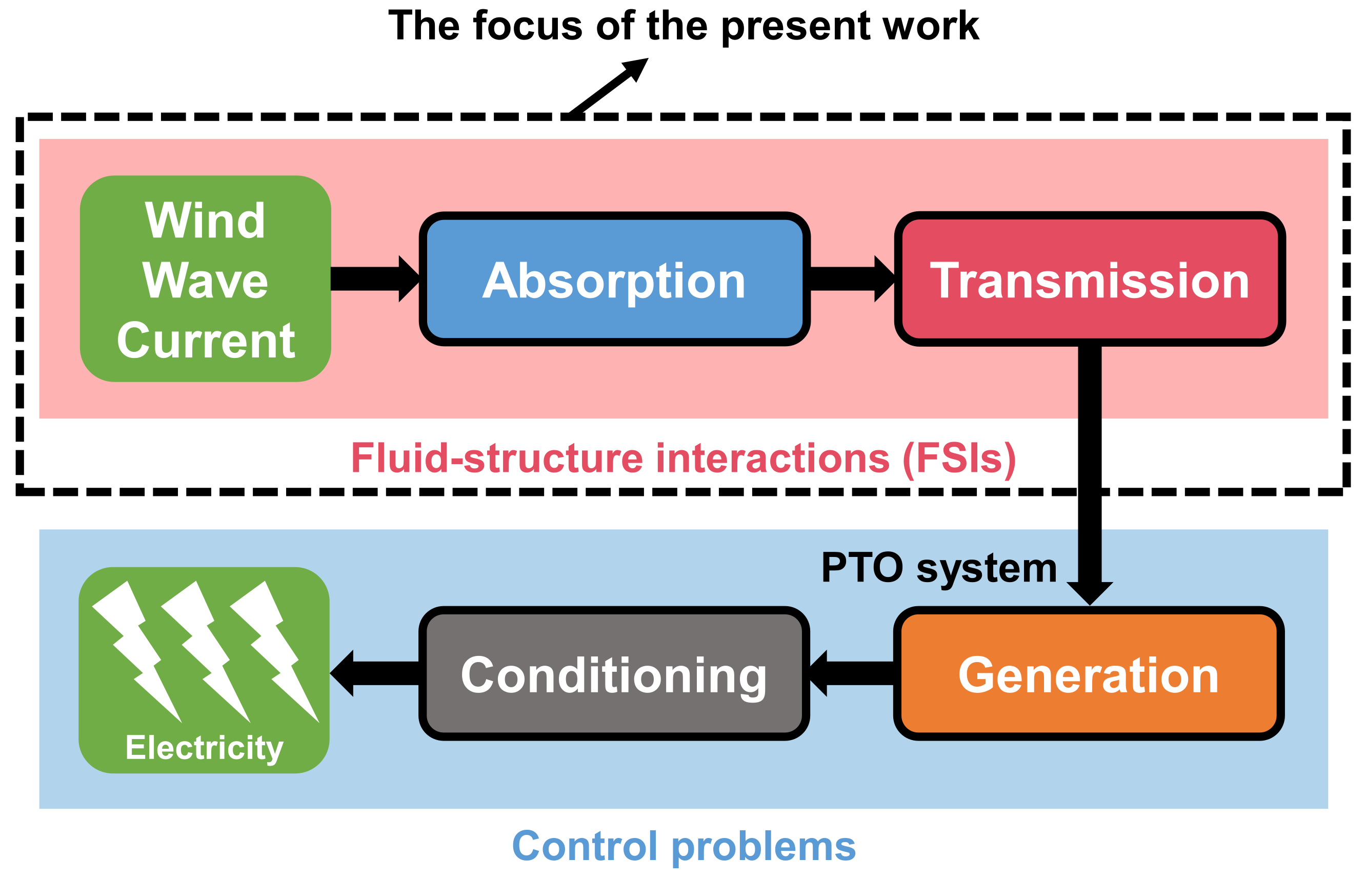
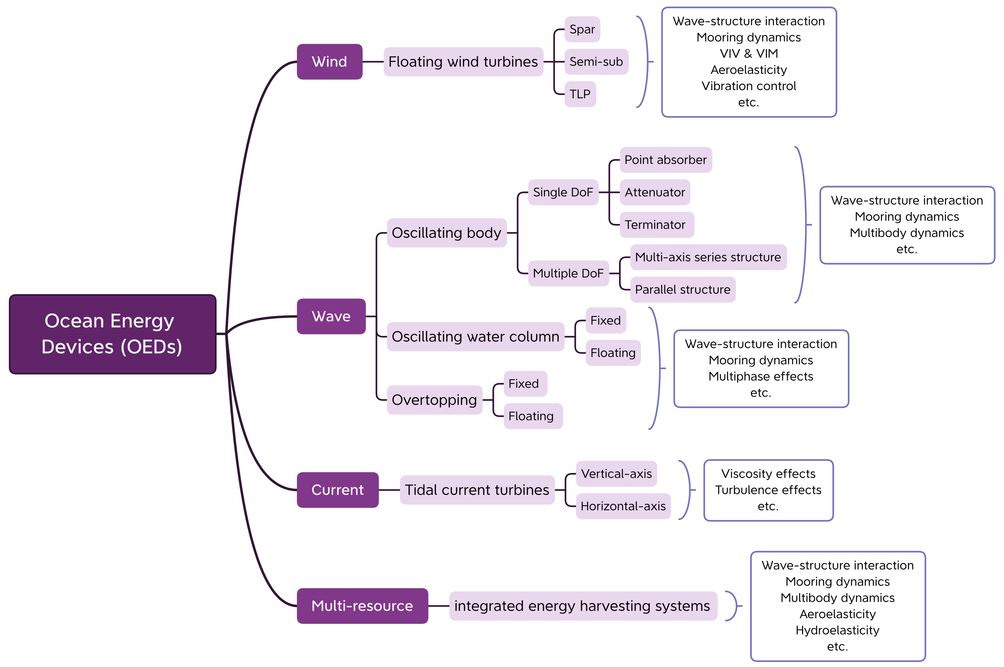
:1. Introduction
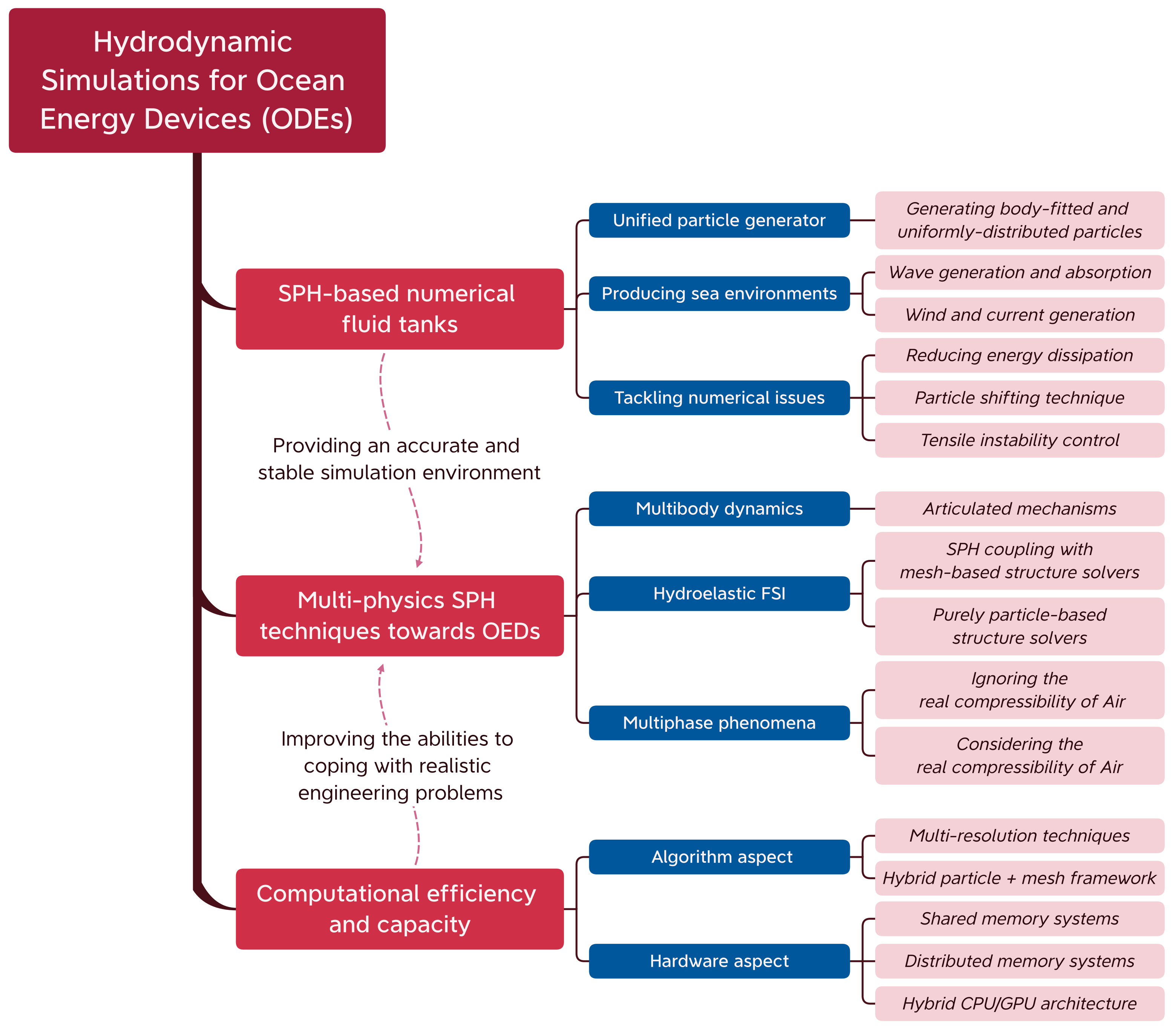
- 1.
- SPH-based numerical fluid tanks.
- 2.
- Multi-physics SPH techniques for simulating OEDs.
- 3.
- Computational efficiency and capacity.
2. A Brief Recall of the SPH Method for Simulating Hydrodynamic Problems Related to OEDs
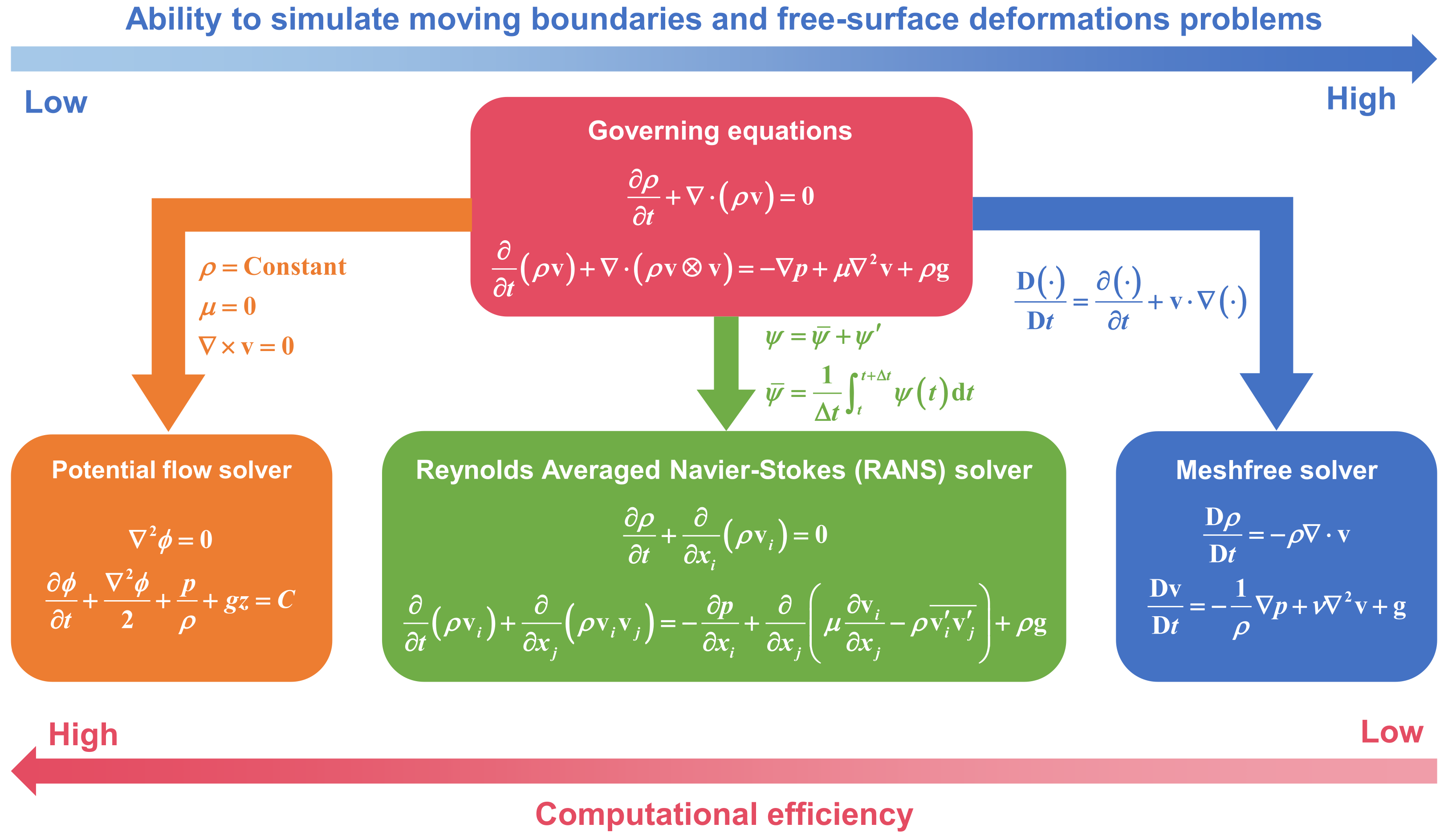
2.1. Governing Equations: Weakly Compressible and Truly Incompressible Hypotheses
2.1.1. Weakly Compressible Hypotheses
2.1.2. Truly Incompressible Hypotheses
2.1.3. Weakly Compressible or Truly Incompressible: The Best Choice towards OEDs Simulations
2.2. The Fundamental Concepts of SPH
2.2.1. Kernel and Particle Approximations
2.2.2. Discrete Governing Equations: The WCSPH Model
2.3. Time Integration
2.4. Boundary Conditions
2.4.1. Free-Surface Boundary Condition
2.4.2. Wall Boundary Condition
3. Numerical Fluid Tank Based on SPH for Simulating Hydrodynamic Problems Related to OEDs
3.1. Wave Tank
3.1.1. Wave Generation
3.1.2. Wave Absorption
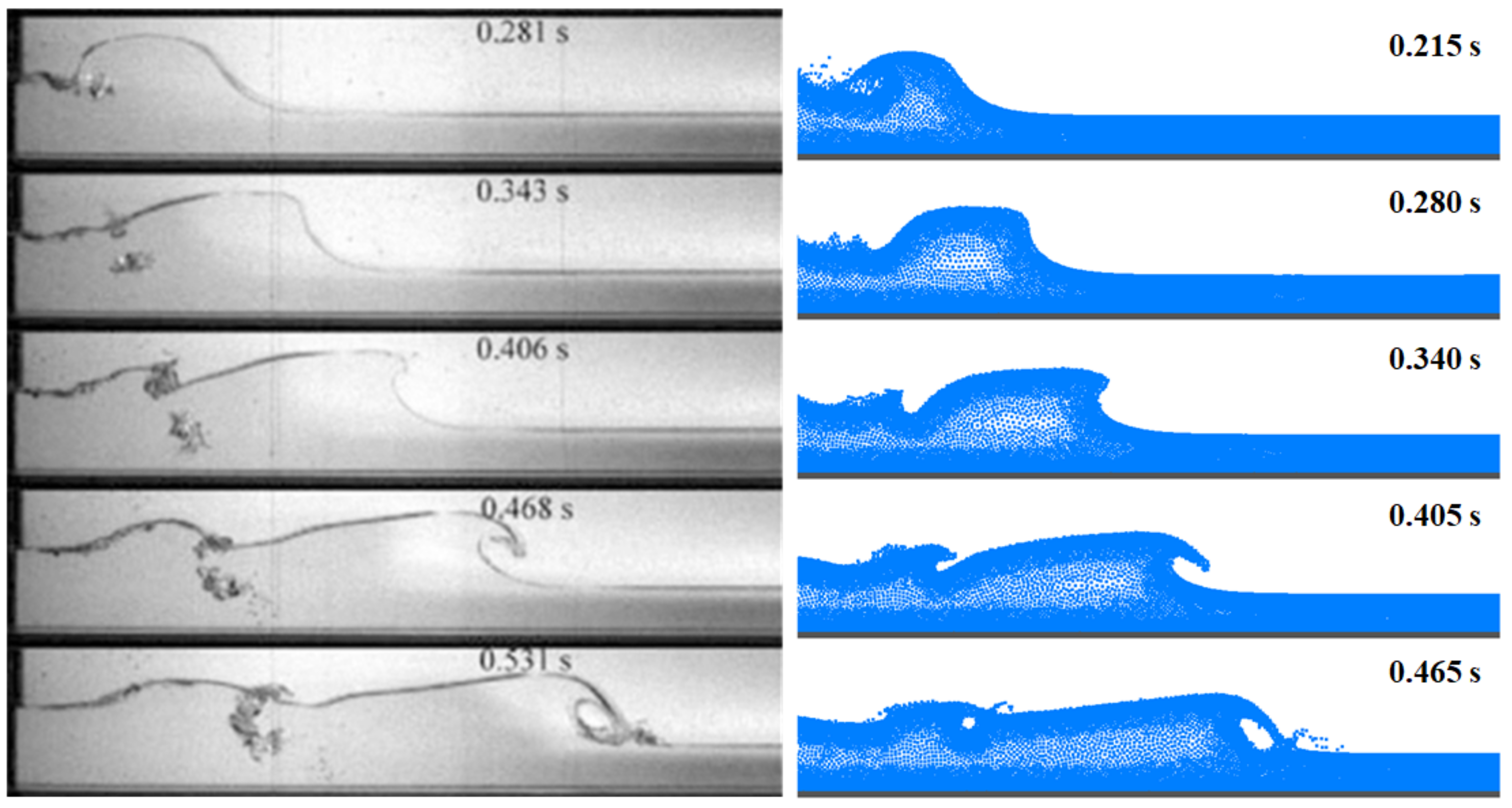
3.1.3. Wave Energy Attenuation
3.2. Current and Wind Tunnels
3.3. Numerical Issues Existing in NFTs
3.3.1. Disordered Particle Distribution: Using Particle-Shifting Techniques
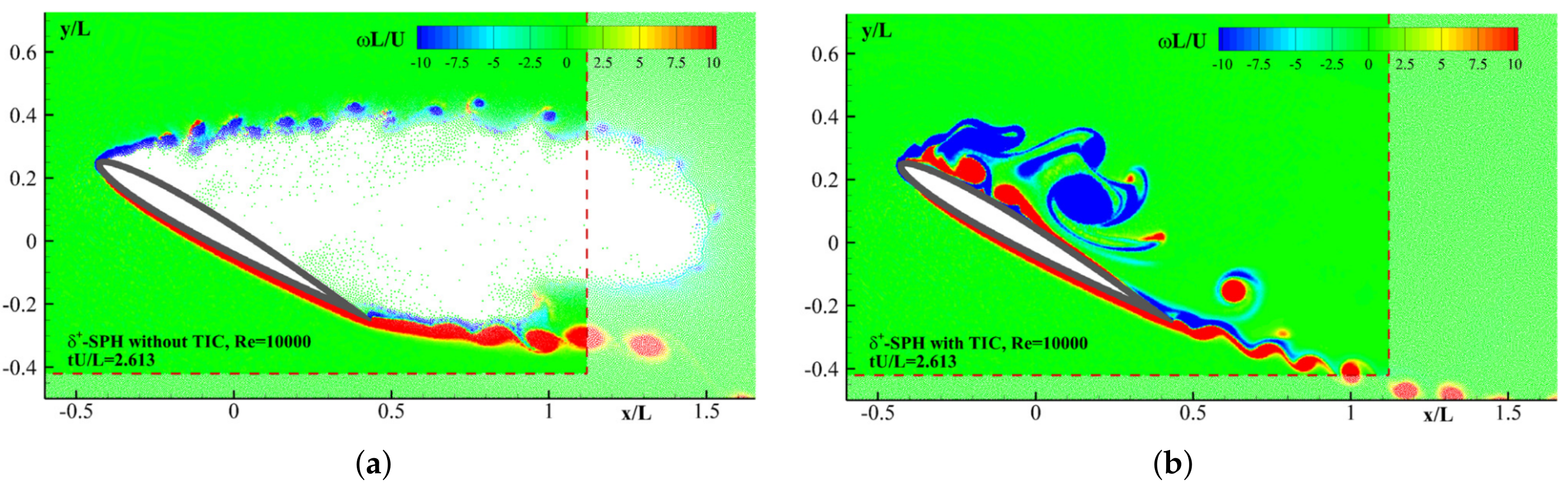
3.3.2. SPH Techniques to Prevent Tensile Instability
4. Multibody Coupling and Mooring Hydrodynamics
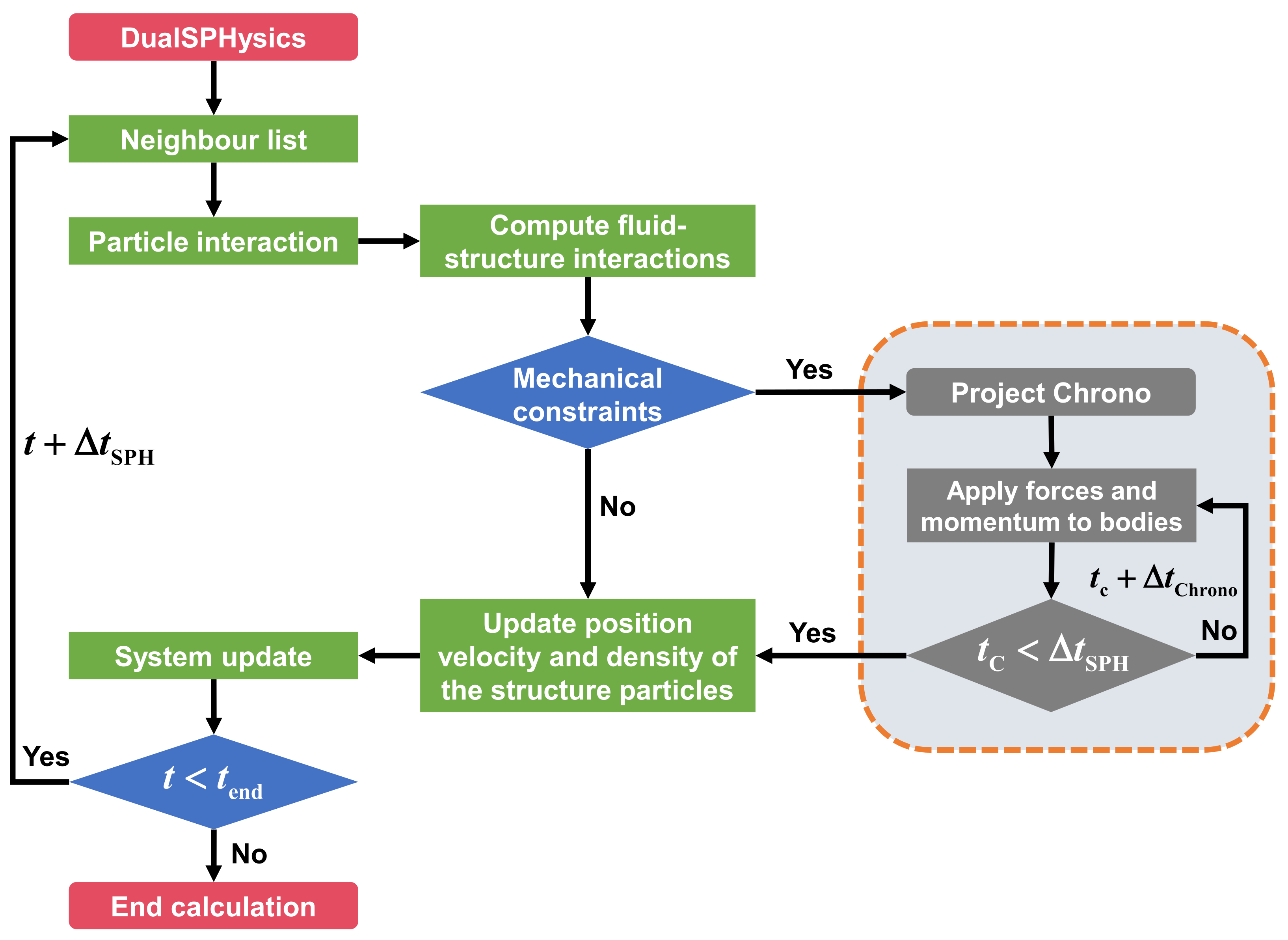
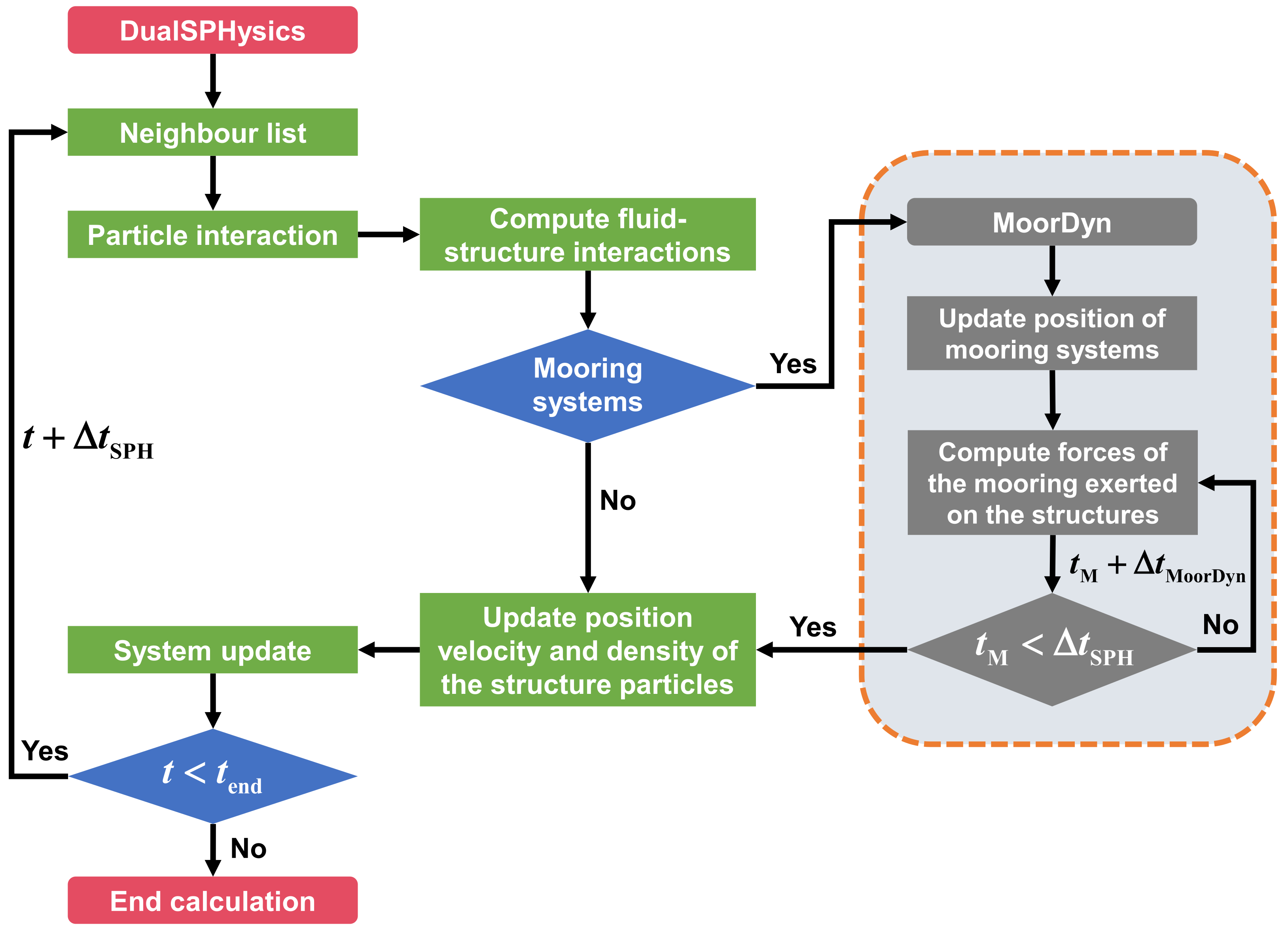
4.1. DualSPHysics’ Solution: Incorporating with Project Chrono and MoorDyn
4.2. SPHinXsys’ Solution: Incorporating with Simbody
5. Hydroelastic Effects in Hydrodynamic Problems Related to OEDs
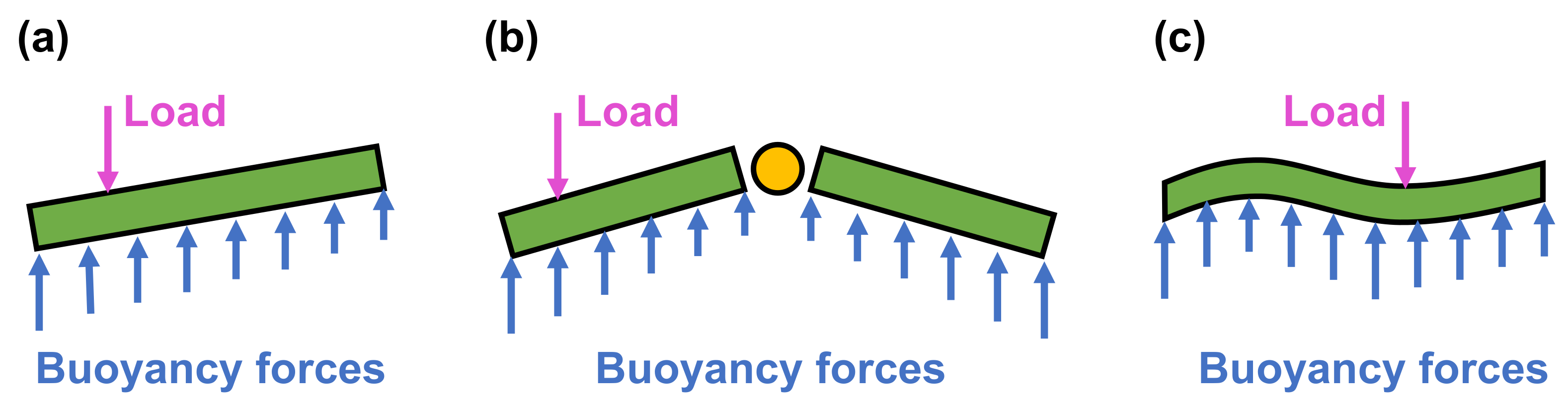
5.1. The Origin of the Flexibility of OEDs
5.2. Coupling Methods between SPH and Other Structure Solvers
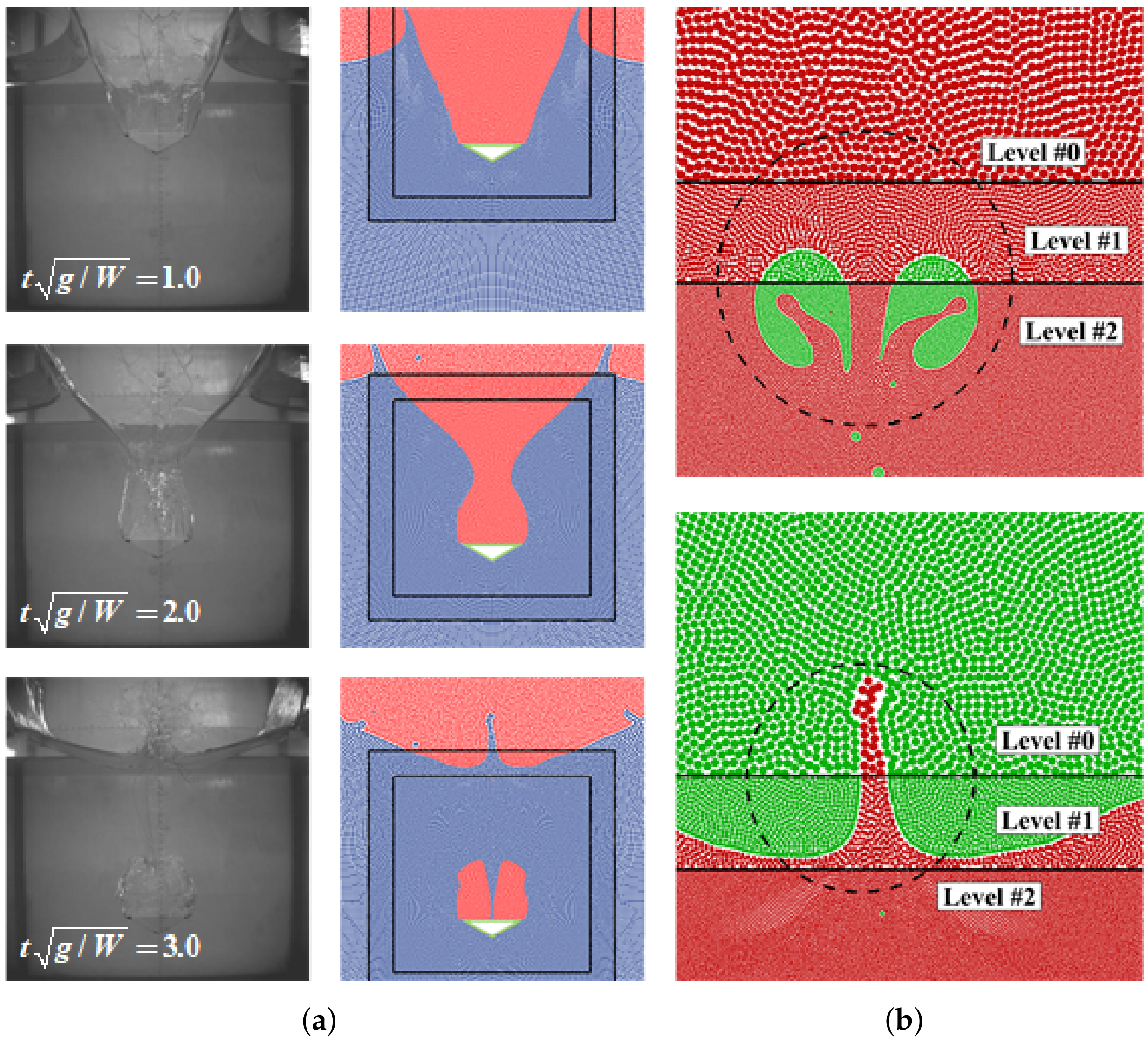
6. Multiphase Effects in Hydrodynamic Problems Related to OEDs
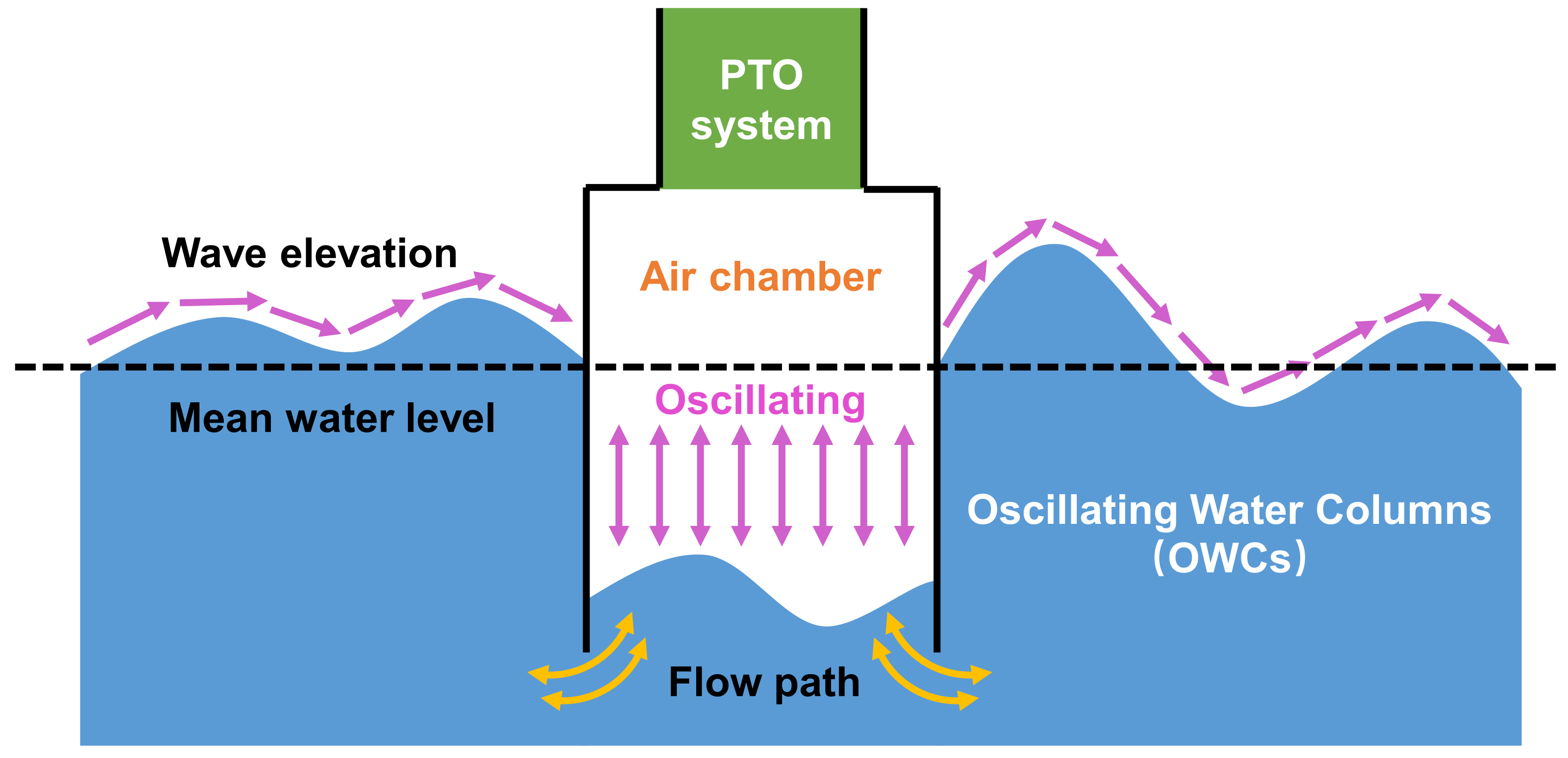
6.1. Multiphase Effects in the OWCs
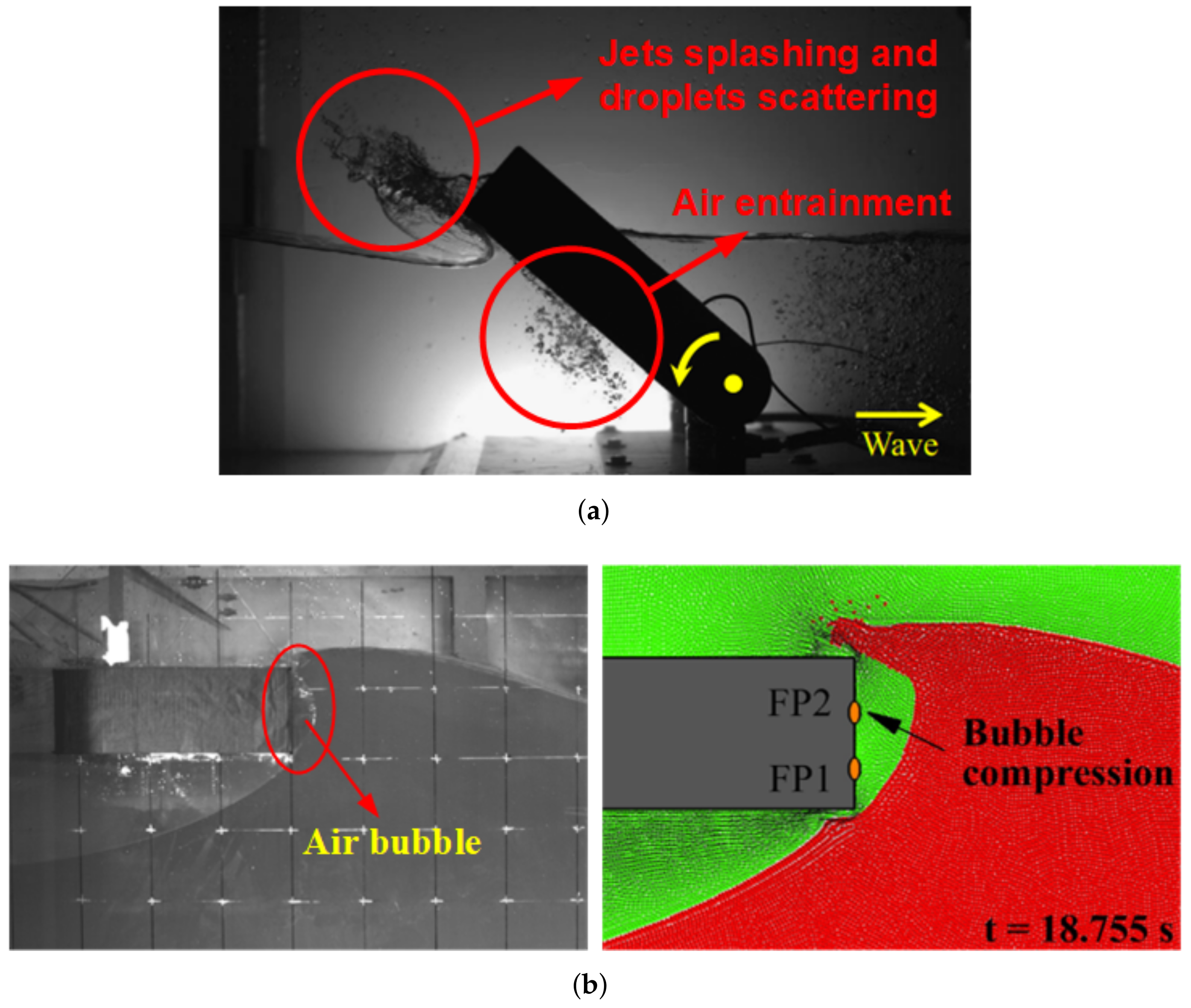
6.2. Air-Cushioning Effects in the Wave Slamming on OEDs
7. Techniques to Improve Numerical Efficiency in SPH Simulations of Hydrodynamic Problems Related to OEDs
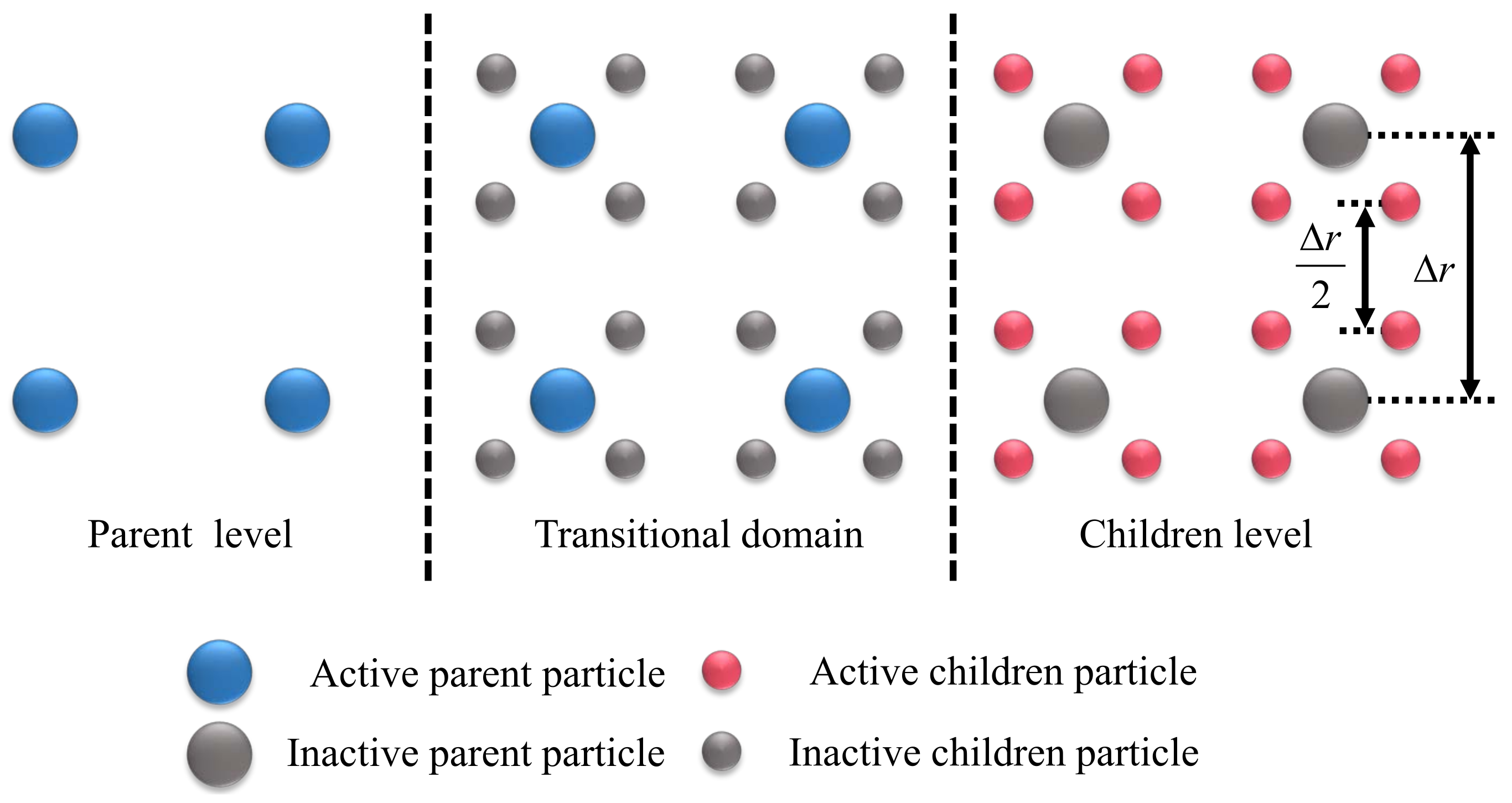
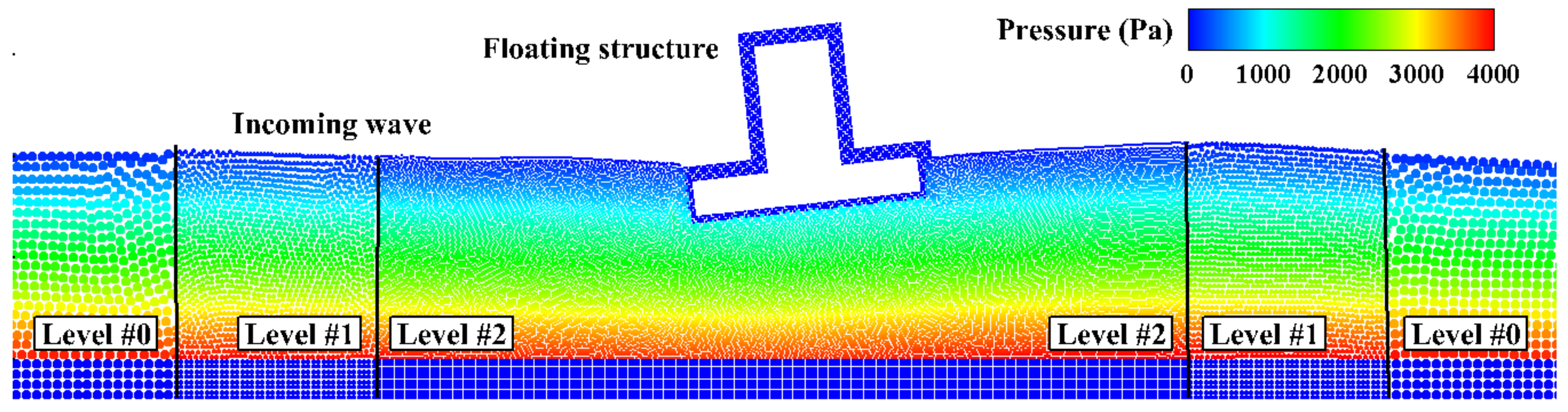
7.1. Multi-Particle-Resolution Techniques
7.1.1. Chiron’s APR Technique
7.1.2. Yang’s ASR Technique
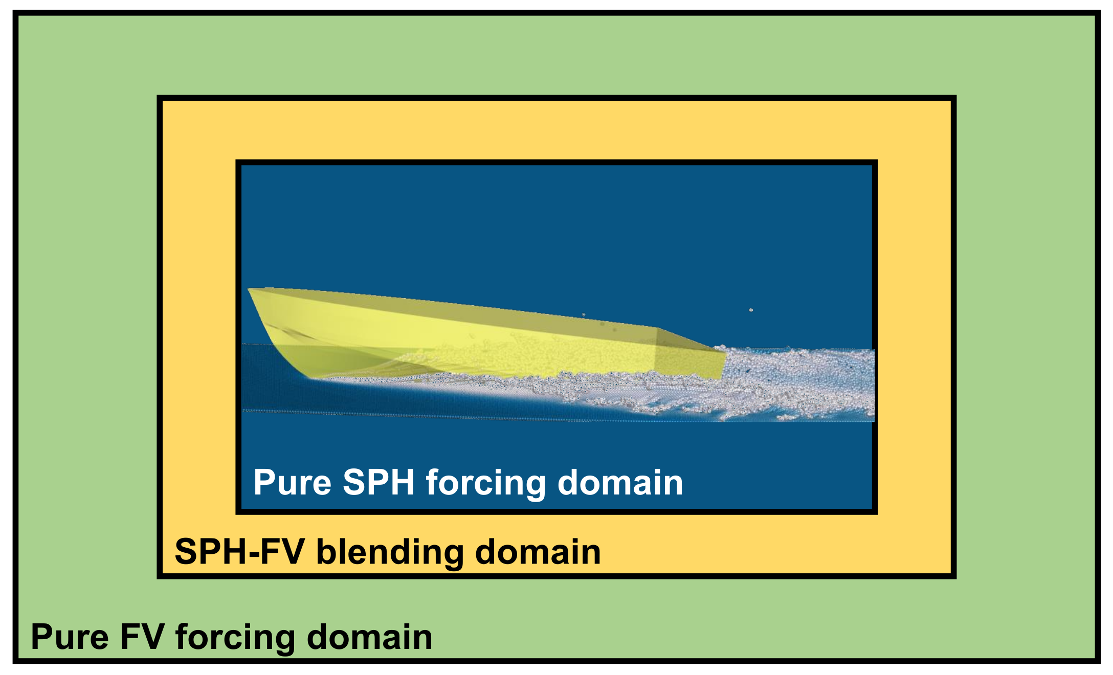
7.2. SPH Coupling with Other Efficient Numerical Methods
7.3. High-Performance Parallel Computing
7.3.1. Accelerating SPH Simulation with Central Processing Units (CPUs)
7.3.2. Accelerating SPH Simulation with Graphics Processing Units (GPUs)
8. Conclusions and Prospects
- High-order accurate SPH models;
- Coupled hydroelasticity-multibody FSI solver;
- Multiphase SPH models of high fidelity and efficiency considering real compressibility;
- Accurate and robust multi-scale particle-mesh coupling solver;
- Turbulence and cavitation modeling in the SPH framework.
Author Contributions
Funding
Acknowledgments
Conflicts of Interest
Abbreviations
| SPH | Smoothed Particle Hydrodynamics |
| CFD | Computational Fluid Dynamics |
| PF | Potential Flow |
| BE | Boundary Element |
| RANS | Reynolds Average Navier Stokes |
| SPHERIC | SPH rEsearch and engineeRing International Community |
| KFSBC | Kinematic Free-surface Boundary Condition |
| DFSBC | Dynamic Free-surface Boundary Condition |
| FV | Finite Volume |
| FD | Finite Differece |
| TI | Tensile Instability |
| PD | Peridynamics |
| VLFS(s) | Very Large Floating Structure(s) |
| MCS(s) | Mechanical Constraint Structure(s) |
| AMR | Adaptive Mesh Refinement |
| ALE | Arbitrary Lagrangian Eulerian |
| KGC | Kernel Gradient Correction |
| DBC | Dynamic Boundary Condition |
| PPA | Particle Packing Algorithm |
| NFT(s) | Numerical Fluid Tank(s) |
| NWT(s) | Numerical Wave Tank(s) |
| MCS(s) | Mechanical Constraint Structure(s) |
| ISPH | Incompressible Smoothed Particle Hydrodynamics |
| WCSPH | Weakly Compressible Smoothed Particle Hydrodynamics |
| TLSPH | Total Lagrangian Smoothed Particle Hydrodynamics |
| RKPM | Reproducing Kernel Particle Method |
| SPIM | Smoothed Point Interpolation Method |
| FSI(s) | Fluid–structure Interaction(s) |
| PTO | Power Take-Off |
| IEHSs(s) | Integrated Energy Harvesting System(s) |
| OED(s) | Ocean Energy Device(s) |
| FWT(s) | Floating Wind Turbine(s) |
| WEC(s) | Wave Energy Converter(s) |
| TCT(s) | Tidal Current Turbine(s) |
| OWC(s) | Oscillating Water Column(s) |
| OWSC(s) | Oscillating Wave Surge Converter(s) |
| VLFS(s) | Very Large Floating Structure(s) |
| SPH | Smoothed Particle Hydrodynamics |
| PST(s) | Particle Shifting Technique(s) |
| TIC | Tensile Instability Control |
| TBB | Thread Building Blocks |
| OpenMP | Open Multi-Processing |
| MPI | Massage Passing Interface |
| CUDA | Compute Unified Device Architecture |
| APR | Adaptive Particle Refinement |
| ASR | Adaptive Spatial Refinement |
| VAS | Volume Adaptive Scheme |
| CPU(s) | Central Processing Unit(s) |
| GPU(s) | Graphics Processing Unit(s) |
| SMS(s) | Shared Memory System(s) |
| DMS(s) | Distributed Memory System(s) |
| EoS | Equation of State |
| VIV&VIM | Vortex-Induced Vibration/Motion |
References
- Ammari, C.; Belatrache, D.; Touhami, B.; Makhloufi, S. Sizing, optimization, control and energy management of hybrid renewable energy system—A review. Energy Built Environ. 2021, in press. [Google Scholar] [CrossRef]
- Melikoglu, M. Current status and future of ocean energy sources: A global review. Ocean Eng. 2018, 148, 563–573. [Google Scholar] [CrossRef]
- Salter, S.H. Wave power. Nature 1974, 249, 720–724. [Google Scholar] [CrossRef]
- Khan, N.; Kalair, A.; Abas, N.; Haider, A. Review of ocean tidal, wave and thermal energy technologies. Renew. Sustain. Energy Rev. 2017, 72, 590–604. [Google Scholar] [CrossRef]
- Zhang, X.; Zheng, S.; Lu, D.; Tian, X. Numerical investigation of the dynamic response and power capture performance of a VLFS with a wave energy conversion unit. Eng. Struct. 2019, 195, 62–83. [Google Scholar] [CrossRef]
- Nguyen, H.P.; Wang, C.M.; Tay, Z.Y.; Luong, V.H. Wave energy converter and large floating platform integration: A review. Ocean Eng. 2020, 213, 107768. [Google Scholar] [CrossRef]
- Cevasco, D.; Koukoura, S.; Kolios, A.J. Reliability, availability, maintainability data review for the identification of trends in offshore wind energy applications. Renew. Sustain. Energy Rev. 2021, 136, 110414. [Google Scholar] [CrossRef]
- Ren, Z.; Verma, A.S.; Li, Y.; Teuwen, J.J.E.; Jiang, Z. Offshore wind turbine operations and maintenance: A state-of-the-art review. Renew. Sustain. Energy Rev. 2021, 144, 110886. [Google Scholar] [CrossRef]
- Rinaldi, G.; Thies, P.R.; Johanning, L. Current Status and Future Trends in the Operation and Maintenance of Offshore Wind Turbines: A Review. Energies 2021, 14, 2484. [Google Scholar] [CrossRef]
- Jiang, Z. Installation of offshore wind turbines: A technical review. Renew. Sustain. Energy Rev. 2021, 139, 110576. [Google Scholar] [CrossRef]
- Santhosh, N.; Baskaran, V.; Amarkarthik, A. A review on front end conversion in ocean wave energy converters. Front. Energy 2015, 9, 297–310. [Google Scholar] [CrossRef]
- Ahamed, R.; McKee, K.; Howard, I. Advancements of wave energy converters based on power take off (PTO) systems: A review. Ocean Eng. 2020, 204, 107248. [Google Scholar] [CrossRef]
- Zhang, Y.; Zhao, Y.; Sun, W.; Li, J. Ocean wave energy converters: Technical principle, device realization, and performance evaluation. Renew. Sustain. Energy Rev. 2021, 141, 110764. [Google Scholar] [CrossRef]
- Qian, P.; Feng, B.; Liu, H.; Tian, X.; Si, Y.; Zhang, D. Review on configuration and control methods of tidal current turbines. Renew. Sustain. Energy Rev. 2019, 108, 125–139. [Google Scholar] [CrossRef]
- Nachtane, M.; Tarfaoui, M.; Goda, I.; Rouway, M. A review on the technologies, design considerations and numerical models of tidal current turbines. Renew. Energy 2020, 157, 1274–1288. [Google Scholar] [CrossRef]
- Chowdhury, M.S.; Rahman, K.S.; Selvanathan, V.; Nuthammachot, N.; Suklueng, M.; Mostafaeipour, A.; Habib, A.; Akhtaruzzaman, M.; Amin, N.; Techato, K. Current trends and prospects of tidal energy technology. Environ. Dev. Sustain. 2021, 23, 8179–8194. [Google Scholar] [CrossRef]
- Said, H.A.; Ringwood, J.V. Grid integration aspects of wave energy—Overview and perspectives. IET Renew. Power Gener. 2021, 15, 3045–3064. [Google Scholar] [CrossRef]
- Ozkop, E.; Altas, I.H. Control, power and electrical components in wave energy conversion systems: A review of the technologies. Renew. Sustain. Energy Rev. 2017, 67, 106–115. [Google Scholar] [CrossRef]
- Penalba, M.; Giorgi, G.; Ringwood, J.V. Mathematical modelling of wave energy converters: A review of nonlinear approaches. Renew. Sustain. Energy Rev. 2017, 78, 1188–1207. [Google Scholar] [CrossRef] [Green Version]
- Chen, Z.; Zhou, B.; Zhang, L.; Li, C.; Zang, J.; Zheng, X.; Xu, J.; Zhang, W. Experimental and numerical study on a novel dual-resonance wave energy converter with a built-in power take-off system. Energy 2018, 165, 1008–1020. [Google Scholar] [CrossRef]
- Zhang, H.; Zhou, B.; Zang, J.; Vogel, C.; Fan, T.; Chen, C. Effects of narrow gap wave resonance on a dual-floater WEC-breakwater hybrid system. Ocean Eng. 2021, 225, 108762. [Google Scholar] [CrossRef]
- Cheng, Y.; Xi, C.; Dai, S.; Ji, C.; Collu, M.; Li, M.; Yuan, Z.; Incecik, A. Wave energy extraction and hydroelastic response reduction of modular floating breakwaters as array wave energy converters integrated into a very large floating structure. Appl. Energy 2022, 306, 117953. [Google Scholar] [CrossRef]
- Hansen, M.O.L.; Sørensen, J.N.; Voutsinas, S.; Sørensen, N.; Madsen, H.A. State of the art in wind turbine aerodynamics and aeroelasticity. Prog. Aerosp. Sci. 2006, 42, 285–330. [Google Scholar] [CrossRef]
- Zhang, P.; Huang, S. Review of aeroelasticity for wind turbine: Current status, research focus and future perspectives. Front. Energy 2011, 5, 419–434. [Google Scholar] [CrossRef]
- Wang, L.; Liu, X.; Kolios, A. State of the art in the aeroelasticity of wind turbine blades: Aeroelastic modelling. Renew. Sustain. Energy Rev. 2016, 64, 195–210. [Google Scholar] [CrossRef] [Green Version]
- Lu, D.; Tian, X.; Lu, W.; Zhang, X. Combined effects of raft length ratio and structural flexibility on power capture performance of an interconnected-two-raft wave energy converter. Ocean Eng. 2019, 177, 12–28. [Google Scholar] [CrossRef]
- Zhang, X.; Lu, D.; Guo, F.; Gao, Y.; Sun, Y. The maximum wave energy conversion by two interconnected floaters: Effects of structural flexibility. Appl. Ocean Res. 2018, 71, 34–47. [Google Scholar] [CrossRef]
- Dias, F.; Ghidaglia, J.M. Slamming: Recent Progress in the Evaluation of Impact Pressures. Annu. Rev. Fluid Mech. 2018, 50, 243–273. [Google Scholar] [CrossRef]
- Saincher, S.; Banerjee, J. Influence of wave breaking on the hydrodynamics of wave energy converters: A review. Renew. Sustain. Energy Rev. 2016, 58, 704–717. [Google Scholar] [CrossRef]
- Sun, H.; Kim, E.S.; Nowakowski, G.; Mauer, E.; Bernitsas, M.M. Effect of mass-ratio, damping, and stiffness on optimal hydrokinetic energy conversion of a single, rough cylinder in flow induced motions. Renew. Energy 2016, 99, 936–959. [Google Scholar] [CrossRef] [Green Version]
- Zhang, B.; Mao, Z.; Song, B.; Ding, W.; Tian, W. Numerical investigation on effect of damping-ratio and mass-ratio on energy harnessing of a square cylinder in FIM. Energy 2018, 144, 218–231. [Google Scholar] [CrossRef]
- Kim, E.S.; Sun, H.; Park, H.; Shin, S.-c.; Chae, E.J.; Ouderkirk, R.; Bernitsas, M.M. Development of an alternating lift converter utilizing flow-induced oscillations to harness horizontal hydrokinetic energy. Renew. Sustain. Energy Rev. 2021, 145, 111094. [Google Scholar] [CrossRef]
- Yang, S.; Chen, H.; Ji, Z.; Li, H.; Xiang, X. Modelling and analysis of inertia self-tuning phase control strategy for a floating multi-body wave energy converter. IET Renew. Power Gener. 2021, 15, 3126–3137. [Google Scholar] [CrossRef]
- Zhang, Y.; Zang, W.; Zheng, J.; Cappietti, L.; Zhang, J.; Zheng, Y.; Fernandez-Rodriguez, E. The influence of waves propagating with the current on the wake of a tidal stream turbine. Appl. Energy 2021, 290, 116729. [Google Scholar] [CrossRef]
- Rahman, M.; Ong, Z.C.; Chong, W.T.; Julai, S.; Khoo, S.Y. Performance enhancement of wind turbine systems with vibration control: A review. Renew. Sustain. Energy Rev. 2015, 51, 43–54. [Google Scholar] [CrossRef]
- Zuo, H.; Bi, K.; Hao, H. A state-of-the-art review on the vibration mitigation of wind turbines. Renew. Sustain. Energy Rev. 2020, 121, 109710. [Google Scholar] [CrossRef]
- Sentchev, A.; Thiébaut, M.; Schmitt, F.G. Impact of turbulence on power production by a free-stream tidal turbine in real sea conditions. Renew. Energy 2020, 147, 1932–1940. [Google Scholar] [CrossRef]
- Ahmadi, M.H.B.; Yang, Z. The evolution of turbulence characteristics in the wake of a horizontal axis tidal stream turbine. Renew. Energy 2020, 151, 1008–1015. [Google Scholar] [CrossRef]
- Ebdon, T.; Allmark, M.J.; O Doherty, D.M.; Mason-Jones, A.; O Doherty, T.; Germain, G.; Gaurier, B. The impact of turbulence and turbine operating condition on the wakes of tidal turbines. Renew. Energy 2021, 165, 96–116. [Google Scholar] [CrossRef]
- Neunaber, I.; Hölling, M.; Whale, J.; Peinke, J. Comparison of the turbulence in the wakes of an actuator disc and a model wind turbine by higher order statistics: A wind tunnel study. Renew. Energy 2021, 179, 1650–1662. [Google Scholar] [CrossRef]
- Davidson, J.; Ringwood, J.V. Mathematical Modelling of Mooring Systems for Wave Energy Converters—A Review. Energies 2017, 10, 666. [Google Scholar] [CrossRef] [Green Version]
- Xu, S.; Wang, S.; Guedes Soares, C. Review of mooring design for floating wave energy converters. Renew. Sustain. Energy Rev. 2019, 111, 595–621. [Google Scholar] [CrossRef]
- Koh, H.J.; Ruy, W.S.; Cho, I.H.; Kweon, H.M. Multi-objective optimum design of a buoy for the resonant-type wave energy converter. J. Mar. Sci. Technol. 2015, 20, 53–63. [Google Scholar] [CrossRef]
- Zhang, Z.Y.; Liu, H.X.; Zhang, L.; Zhang, W.C.; Ma, Q.W. Study on the performance analysis and optimization of funnel concept in wave-energy conversion. J. Mar. Sci. Technol. 2018, 23, 696–705. [Google Scholar] [CrossRef]
- Wei, Y.; Rafiee, A.; Henry, A.; Dias, F. Wave interaction with an oscillating wave surge converter, Part I: Viscous effects. Ocean Eng. 2015, 104, 185–203. [Google Scholar] [CrossRef]
- Wei, Y.; Abadie, T.; Henry, A.; Dias, F. Wave interaction with an Oscillating Wave Surge Converter. Part II: Slamming. Ocean Eng. 2016, 113, 319–334. [Google Scholar] [CrossRef]
- Henderson, R. Design, simulation, and testing of a novel hydraulic power take-off system for the Pelamis wave energy converter. Renew. Energy 2006, 31, 271–283. [Google Scholar] [CrossRef]
- Kofoed, J.P.; Frigaard, P.; Friis-Madsen, E.; Sørensen, H.C. Prototype testing of the wave energy converter wave dragon. Renew. Energy 2006, 31, 181–189. [Google Scholar] [CrossRef] [Green Version]
- Ning, D.; Zhao, X.; Göteman, M.; Kang, H. Hydrodynamic performance of a pile-restrained WEC-type floating breakwater: An experimental study. Renew. Energy 2016, 95, 531–541. [Google Scholar] [CrossRef]
- Chen, L.; Hashim, R.; Othman, F.; Motamedi, S. Experimental study on scour profile of pile-supported horizontal axis tidal current turbine. Renew. Energy 2017, 114, 744–754. [Google Scholar] [CrossRef]
- Xu, X.; Day, S. Experimental investigation on dynamic responses of a spar-type offshore floating wind turbine and its mooring system behaviour. Ocean Eng. 2021, 236, 109488. [Google Scholar] [CrossRef]
- Windt, C.; Davidson, J.; Ringwood, J.V. Numerical analysis of the hydrodynamic scaling effects for the Wavestar wave energy converter. J. Fluids Struct. 2021, 105, 103328. [Google Scholar] [CrossRef]
- Palm, J.; Eskilsson, C.; Bergdahl, L.; Bensow, R.E. Assessment of Scale Effects, Viscous Forces and Induced Drag on a Point-Absorbing Wave Energy Converter by CFD Simulations. J. Mar. Sci. Eng. 2018, 6, 124. [Google Scholar] [CrossRef] [Green Version]
- Dai, S.; Day, S.; Yuan, Z.; Wang, H. Investigation on the hydrodynamic scaling effect of an OWC type wave energy device using experiment and CFD simulation. Renew. Energy 2019, 142, 184–194. [Google Scholar] [CrossRef]
- Ransley, E.; Greaves, D.; Raby, A.; Simmonds, D.; Hann, M. Survivability of wave energy converters using CFD. Renew. Energy 2017, 109, 235–247. [Google Scholar] [CrossRef] [Green Version]
- Nuernberg, M.; Tao, L. Three dimensional tidal turbine array simulations using OpenFOAM with dynamic mesh. Ocean Eng. 2018, 147, 629–646. [Google Scholar] [CrossRef] [Green Version]
- Chen, J.; Hu, Z.; Wan, D.; Xiao, Q. Comparisons of the dynamical characteristics of a semi-submersible floating offshore wind turbine based on two different blade concepts. Ocean Eng. 2018, 153, 305–318. [Google Scholar] [CrossRef] [Green Version]
- Fertahi, E.D.; Bouhal, T.; Rajad, O.; Kousksou, T.; Arid, A.; El Rhafiki, T.; Jamil, A.; Benbassou, A. CFD performance enhancement of a low cut-in speed current Vertical Tidal Turbine through the nested hybridization of Savonius and Darrieus. Energy Convers. Manag. 2018, 169, 266–278. [Google Scholar] [CrossRef]
- Cheng, P.; Huang, Y.; Wan, D. A numerical model for fully coupled aero-hydrodynamic analysis of floating offshore wind turbine. Ocean Eng. 2019, 173, 183–196. [Google Scholar] [CrossRef]
- Faltinsen, O. Sea Loads on Ships and Offshore Structures (Cambridge Ocean Technology Series); Cambridge University Press: Cambridge, UK, 1993. [Google Scholar]
- Versteeg, H.K.; Malalasekera, W. An Introduction to Computational Fluid Dynamics: The Finite Volume Method, 2nd ed.; Prentice Hall: Harlow, UK, 2007. [Google Scholar]
- Liu, G.R.; Liu, M.B. Smoothed Particle Hydrodynamics: A Meshfree Particle Method; World Scientific Publishing Company: Singapore, 2003. [Google Scholar]
- Gingold, R.A.; Monaghan, J.J. Smoothed particle hydrodynamics: Theory and application to non-spherical stars. Mon. Not. R. Astron. Soc. 1977, 181, 375–389. [Google Scholar] [CrossRef]
- Lucy, L.B. A numerical approach to the testing of the fission hypothesis. Astrophys. J. 1977, 8, 1013–1024. [Google Scholar] [CrossRef]
- Monaghan, J.J. Simulating Free Surface Flows with SPH. J. Comput. Phys. 1994, 110, 399–406. [Google Scholar] [CrossRef]
- Gotoh, H.; Khayyer, A. On the state-of-the-art of particle methods for coastal and ocean engineering. Coast. Eng. J. 2018, 60, 79–103. [Google Scholar] [CrossRef]
- Luo, M.; Khayyer, A.; Lin, P. Particle methods in ocean and coastal engineering. Appl. Ocean Res. 2021, 114, 102734. [Google Scholar] [CrossRef]
- Gomez-Gesteira, M.; Rogers, B.D.; Violeau, D.; Grassa, J.M.; Crespo, A.J.C. Foreword: SPH for free-surface flows. J. Hydraul. Res. 2010, 48, 3–5. [Google Scholar] [CrossRef]
- Violeau, D.; Rogers, B.D. Smoothed particle hydrodynamics (SPH) for free-surface flows: Past, present and future. J. Hydraul. Res. 2015, 54, 1–26. [Google Scholar] [CrossRef]
- Ren, L.; Wang, X.; Zhang, Y.; Gu, S. SPH method-based study on energy dissipation characteristics of stepped spillway. Water Resour. Hydropower Eng. 2017, 48, 113–117. [Google Scholar]
- Sun, P.; Zhang, A.M.; Marrone, S.; Ming, F. An accurate and efficient SPH modeling of the water entry of circular cylinders. Appl. Ocean Res. 2018, 72, 60–75. [Google Scholar] [CrossRef]
- He, F.; Zhang, H.; Huang, C.; Liu, M. Numerical investigation of the solitary wave breaking over a slope by using the finite particle method. Coast. Eng. 2020, 156, 103617. [Google Scholar] [CrossRef]
- Wang, Z.B.; Chen, R.; Wang, H.; Liao, Q.; Zhu, X.; Li, S.Z. An overview of smoothed particle hydrodynamics for simulating multiphase flow. Appl. Math. Model. 2016, 40, 9625–9655. [Google Scholar] [CrossRef]
- Zhang, A.m.; Sun, P.n.; Ming, F.r.; Colagrossi, A. Smoothed particle hydrodynamics and its applications in fluid-structure interactions. J. Hydrodyn. Ser. B 2017, 29, 187–216. [Google Scholar] [CrossRef]
- Liu, M.; Zhang, Z. Smoothed particle hydrodynamics (SPH) for modeling fluid-structure interactions. Sci. China Phys. Mech. Astron. 2019, 62, 984701. [Google Scholar] [CrossRef]
- Zhang, G.; Zhao, W.; Wan, D. Partitioned MPS-FEM method for free-surface flows interacting with deformable structures. Appl. Ocean Res. 2021, 114, 102775. [Google Scholar] [CrossRef]
- Gotoh, H.; Khayyer, A.; Shimizu, Y. Entirely Lagrangian meshfree computational methods for hydroelastic fluid-structure interactions in ocean engineering—Reliability, adaptivity and generality. Appl. Ocean Res. 2021, 115, 102822. [Google Scholar] [CrossRef]
- Liu, M.B.; Liu, G.R. Smoothed Particle Hydrodynamics (SPH): An Overview and Recent Developments. Arch. Comput. Methods Eng. 2010, 17, 25–76. [Google Scholar] [CrossRef] [Green Version]
- Monaghan, J.J. Smoothed Particle Hydrodynamics and Its Diverse Applications. Annu. Rev. Fluid Mech. 2012, 44, 323–346. [Google Scholar] [CrossRef]
- Shadloo, M.S.; Oger, G.; Le Touzé, D. Smoothed particle hydrodynamics method for fluid flows, towards industrial applications: Motivations, current state, and challenges. Comput. Fluids 2016, 136, 11–34. [Google Scholar] [CrossRef]
- Zhang, H.; Qu, X. SPH method-based study on numerical simulation of jet flow. Water Resour. Hydropower Eng. 2017, 48, 82–85. [Google Scholar]
- Ye, T.; Pan, D.; Huang, C.; Liu, M. Smoothed particle hydrodynamics (SPH) for complex fluid flows: Recent developments in methodology and applications. Phys. Fluids 2019, 31, 11301. [Google Scholar] [CrossRef]
- Oger, G.; Vergnaud, A.; Bouscasse, B.; Ohana, J.; Zarim, M.A.; De Leffe, M.; Bannier, A.; Chiron, L.; Jus, Y.; Garnier, M.; et al. Simulations of helicopter ditching using smoothed particle hydrodynamics. J. Hydrodyn. 2020, 32, 653–663. [Google Scholar] [CrossRef]
- Violeau, D. Fluid Mechanics and the SPH Method: Theory and Applications; Oxford University Press: Oxford, UK, 2012. [Google Scholar]
- Monaghan, J.J. Smoothed particle hydrodynamics. Rep. Prog. Phys. 2005, 68, 1703–1759. [Google Scholar] [CrossRef]
- Colagrossi, A.; Landrini, M. Numerical simulation of interfacial flows by smoothed particle hydrodynamics. J. Comput. Phys. 2003, 191, 448–475. [Google Scholar] [CrossRef]
- Lyu, H.G.; Deng, R.; Sun, P.N.; Miao, J.M. Study on the wedge penetrating fluid interfaces characterized by different density-ratios: Numerical investigations with a multi-phase SPH model. Ocean Eng. 2021, 237, 109538. [Google Scholar] [CrossRef]
- Morris, J.P.; Fox, P.J.; Zhu, Y. Modeling Low Reynolds Number Incompressible Flows Using SPH. J. Comput. Phys. 1997, 136, 214–226. [Google Scholar] [CrossRef]
- Cummins, S.J.; Rudman, M. An SPH Projection Method. J. Comput. Phys. 1999, 152, 584–607. [Google Scholar] [CrossRef]
- Khayyer, A.; Gotoh, H.; Shao, S.D. Corrected Incompressible SPH method for accurate water-surface tracking in breaking waves. Coast. Eng. 2008, 55, 236–250. [Google Scholar] [CrossRef] [Green Version]
- Lee, E.S.; Moulinec, C.; Xu, R.; Violeau, D.; Laurence, D.; Stansby, P. Comparisons of weakly compressible and truly incompressible algorithms for the SPH mesh free particle method. J. Comput. Phys. 2008, 227, 8417–8436. [Google Scholar] [CrossRef]
- Lind, S.J.; Xu, R.; Stansby, P.K.; Rogers, B.D. Incompressible smoothed particle hydrodynamics for free-surface flows: A generalised diffusion-based algorithm for stability and validations for impulsive flows and propagating waves. J. Comput. Phys. 2012, 231, 1499–1523. [Google Scholar] [CrossRef]
- Khayyer, A.; Gotoh, H.; Shimizu, Y. Comparative study on accuracy and conservation properties of two particle regularization schemes and proposal of an optimized particle shifting scheme in ISPH context. J. Comput. Phys. 2017, 332, 236–256. [Google Scholar] [CrossRef]
- Chorin, A.J. Numerical solution of the navier-stokes equations. Math. Comput. 1968, 22, 745–762. [Google Scholar] [CrossRef]
- Khayyer, A.; Gotoh, H.; Shao, S. Enhanced predictions of wave impact pressure by improved incompressible SPH methods. Appl. Ocean Res. 2009, 31, 111–131. [Google Scholar] [CrossRef] [Green Version]
- Khayyer, A.; Gotoh, H. A higher order Laplacian model for enhancement and stabilization of pressure calculation by the MPS method. Appl. Ocean Res. 2010, 32, 124–131. [Google Scholar] [CrossRef]
- Monaghan, J.J.; Gingold, R.A. Shock simulation by the particle method SPH. J. Comput. Phys. 1983, 52, 374–389. [Google Scholar] [CrossRef]
- Antuono, M.; Colagrossi, A.; Marrone, S.; Molteni, D. Free-surface flows solved by means of SPH schemes with numerical diffusive terms. Comput. Phys. Commun. 2010, 181, 532–549. [Google Scholar] [CrossRef]
- Antuono, M.; Colagrossi, A.; Marrone, S. Numerical diffusive terms in weakly-compressible SPH schemes. Comput. Phys. Commun. 2012, 183, 2570–2580. [Google Scholar] [CrossRef]
- Molteni, D.; Colagrossi, A. A simple procedure to improve the pressure evaluation in hydrodynamic context using the SPH. Comput. Phys. Commun. 2009, 180, 861–872. [Google Scholar] [CrossRef]
- Marrone, S.; Antuono, M.; Colagrossi, A.; Colicchio, G.; Le Touzé, D.; Graziani, G. δ-SPH model for simulating violent impact flows. Comput. Methods Appl. Mech. Eng. 2011, 200, 1526–1542. [Google Scholar] [CrossRef]
- Vacondio, R.; Altomare, C.; De Leffe, M.; Hu, X.; Le Touzé, D.; Lind, S.; Marongiu, J.C.; Marrone, S.; Rogers, B.D.; Souto-Iglesias, A. Grand challenges for Smoothed Particle Hydrodynamics numerical schemes. Comput. Part. Mech. 2020, 8, 575–588. [Google Scholar] [CrossRef]
- Colagrossi, A.; Antuono, M.; Le Touzé, D. Theoretical considerations on the free-surface role in the smoothed-particle-hydrodynamics model. Phys. Review. E Stat. Nonlinear Soft Matter Phys. 2009, 79, 056701. [Google Scholar] [CrossRef] [PubMed]
- Chow, A.D.; Rogers, B.D.; Lind, S.J.; Stansby, P.K. Incompressible SPH (ISPH) with fast Poisson solver on a GPU. Comput. Phys. Commun. 2018, 226, 81–103. [Google Scholar] [CrossRef]
- Qiu, L.C. OpenCL-Based GPU Acceleration of ISPH Simulation for Incompressible Flows. Appl. Mech. Mater. 2014, 444–445, 380–384. [Google Scholar] [CrossRef]
- Chow, A.D.; Rogers, B.D.; Lind, S.J.; Stansby, P.K. Numerical wave basin using incompressible smoothed particle hydrodynamics (ISPH) on a single GPU with vertical cylinder test cases. Comput. Fluids 2019, 179, 543–562. [Google Scholar] [CrossRef]
- Crespo, A.J.C.; Domínguez, J.M.; Rogers, B.D.; Gómez-Gesteira, M.; Longshaw, S.; Canelas, R.; Vacondio, R.; Barreiro, A.; García-Feal, O. DualSPHysics: Open-source parallel CFD solver based on Smoothed Particle Hydrodynamics (SPH). Comput. Phys. Commun. 2015, 187, 204–216. [Google Scholar] [CrossRef]
- Bilotta, G.; Hérault, A.; Cappello, A.; Ganci, G.; Del Negro, C. GPUSPH: A Smoothed Particle Hydrodynamics model for the thermal and rheological evolution of lava flows. Geol. Soc. Lond. Spec. Publ. 2016, 426, 387–408. [Google Scholar] [CrossRef]
- Randles, P.W.; Libersky, L.D. Smoothed Particle Hydrodynamics: Some recent improvements and applications. Comput. Methods Appl. Mech. Eng. 1996, 139, 375–408. [Google Scholar] [CrossRef]
- VILA, J.P. On particle weighted methods and smooth particle hydrodynamics. Math. Model. Methods Appl. Sci. 1999, 09, 161–209. [Google Scholar] [CrossRef]
- Zhang, C.; Hu, X.Y.; Adams, N.A. A weakly compressible SPH method based on a low-dissipation Riemann solver. J. Comput. Phys. 2017, 335, 605–620. [Google Scholar] [CrossRef]
- Zhang, C.; Rezavand, M.; Zhu, Y.; Yu, Y.; Wu, D.; Zhang, W.; Wang, J.; Hu, X. SPHinXsys: An open-source multi-physics and multi-resolution library based on smoothed particle hydrodynamics. Comput. Phys. Commun. 2021, 267, 108066. [Google Scholar] [CrossRef]
- Meng, Z.F.; Zhang, A.M.; Wang, P.P.; Ming, F.R. A shock-capturing scheme with a novel limiter for compressible flows solved by smoothed particle hydrodynamics. Comput. Methods Appl. Mech. Eng. 2021, 386, 114082. [Google Scholar] [CrossRef]
- Meng, Z.F.; Ming, F.R.; Wang, P.P.; Zhang, A.M. Numerical simulation of water entry problems considering air effect using a multiphase Riemann-SPH model. Adv. Aerodyn. 2021, 3, 1–16. [Google Scholar]
- The NextFlow Software. Available online: https://www.nextflow-software.com/ (accessed on 25 November 2021).
- Sun, P.; Ming, F.; Zhang, A. Numerical simulation of interactions between free surface and rigid body using a robust SPH method. Ocean Eng. 2015, 98, 32–49. [Google Scholar] [CrossRef]
- Ming, F.R.; Sun, P.N.; Zhang, A.M. Numerical investigation of rising bubbles bursting at a free surface through a multiphase SPH model. Meccanica 2017, 52, 2665–2684. [Google Scholar] [CrossRef]
- Sun, P.N.; Colagrossi, A.; Marrone, S.; Zhang, A.M. The deltaplus-SPH model: Simple procedures for a further improvement of the SPH scheme. Comput. Methods Appl. Mech. Eng. 2017, 315, 25–49. [Google Scholar] [CrossRef]
- Lyu, H.G.; Sun, P.N.; Huang, X.T.; Chen, S.H.; Zhang, A.M. On removing the numerical instability induced by negative pressures in SPH simulations of typical fluid–structure interaction problems in ocean engineering. Appl. Ocean Res. 2021, 117, 102938. [Google Scholar] [CrossRef]
- Domínguez, J.M.; Fourtakas, G.; Altomare, C.; Canelas, R.B.; Tafuni, A.; García-Feal, O.; Martínez-Estévez, I.; Mokos, A.; Vacondio, R.; Crespo, A.J.C.; et al. DualSPHysics: From fluid dynamics to multiphysics problems. Comput. Part. Mech. 2021, 8, 1–29. [Google Scholar] [CrossRef]
- Adami, S.; Hu, X.; Adams, N. A generalized wall boundary condition for smoothed particle hydrodynamics. J. Comput. Phys. 2012, 231, 7057–7075. [Google Scholar] [CrossRef]
- Crespo, A.J.C.; Gómez-Gesteira, M.; Dalrymple, R.A. Boundary Conditions Generated by Dynamic Particles in SPH Methods. Comput. Mater. Contin. 2007, 5, 173–184. [Google Scholar]
- English, A.; Domínguez, J.M.; Vacondio, R.; Crespo, A.J.C.; Stansby, P.K.; Lind, S.J.; Chiapponi, L.; Gómez-Gesteira, M. Modified dynamic boundary conditions (mDBC) for general-purpose smoothed particle hydrodynamics (SPH): Application to tank sloshing, dam break and fish pass problems. Comput. Part. Mech. 2021, 8, 1–15. [Google Scholar] [CrossRef]
- The Dive Solution. Available online: https://www.dive-solutions.de/ (accessed on 25 November 2021).
- Chiron, L.; de Leffe, M.; Oger, G.; Le Touzé, D. Fast and accurate SPH modelling of 3D complex wall boundaries in viscous and non viscous flows. Comput. Phys. Commun. 2019, 234, 93–111. [Google Scholar] [CrossRef]
- Jasak, H. OpenFOAM: Open source CFD in research and industry. Int. J. Nav. Archit. Ocean Eng. 2009, 1, 89–94. [Google Scholar] [CrossRef] [Green Version]
- Si, H. TetGen, a Delaunay-Based Quality Tetrahedral Mesh Generator. ACM Trans. Math. Softw. 2015, 41, 1–36. [Google Scholar] [CrossRef]
- Colagrossi, A.; Bouscasse, B.; Antuono, M.; Marrone, S. Particle packing algorithm for SPH schemes. Comput. Phys. Commun. 2012, 183, 1641–1653. [Google Scholar] [CrossRef] [Green Version]
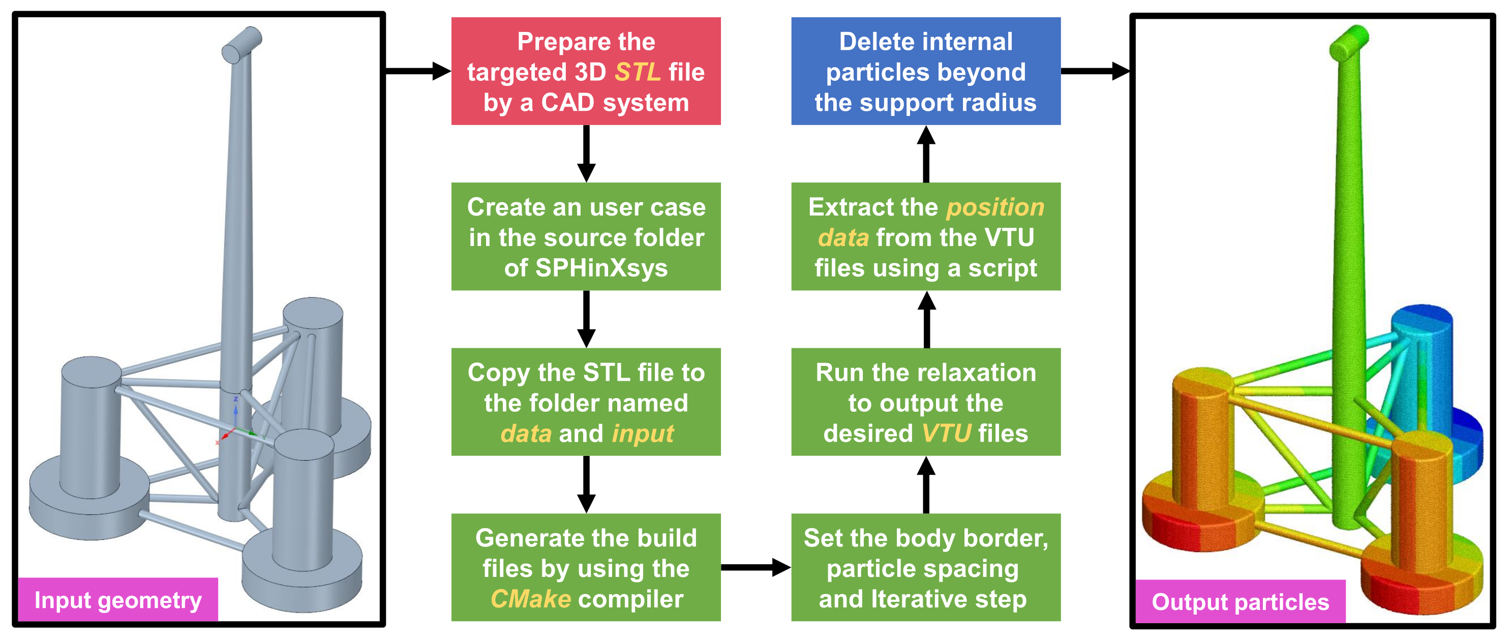
- Zhu, Y.; Zhang, C.; Yu, Y.; Hu, X. A CAD-compatible body-fitted particle generator for arbitrarily complex geometry and its application to wave-structure interaction. J. Hydrodyn. 2021, 33, 195–206. [Google Scholar] [CrossRef]
- Windt, C.; Davidson, J.; Ringwood, J.V. High-fidelity numerical modelling of ocean wave energy systems: A review of computational fluid dynamics-based numerical wave tanks. Renew. Sustain. Energy Rev. 2018, 93, 610–630. [Google Scholar] [CrossRef] [Green Version]
- Higuera, P.; Losada, I.J.; Lara, J.L. Three-dimensional numerical wave generation with moving boundaries. Coast. Eng. 2015, 101, 35–47. [Google Scholar] [CrossRef]
- Liu, X.; Lin, P.; Shao, S. ISPH wave simulation by using an internal wave maker. Coast. Eng. 2015, 95, 160–170. [Google Scholar] [CrossRef] [Green Version]
- Wen, H.; Ren, B. A non-reflective spectral wave maker for SPH modeling of nonlinear wave motion. Wave Motion 2018, 79, 112–128. [Google Scholar] [CrossRef]
- Altomare, C.; Domínguez, J.M.; Crespo, A.J.C.; González-Cao, J.; Suzuki, T.; Gómez-Gesteira, M.; Troch, P. Long-crested wave generation and absorption for SPH-based DualSPHysics model. Coast. Eng. 2017, 127, 37–54. [Google Scholar] [CrossRef]
- Zhang, C.; Wei, Y.; Dias, F.; Hu, X. An efficient fully Lagrangian solver for modeling wave interaction with oscillating wave surge converter. Ocean Eng. 2021, 236, 109540. [Google Scholar] [CrossRef]
- He, M.; Khayyer, A.; Gao, X.; Xu, W.; Liu, B. Theoretical method for generating solitary waves using plunger-type wavemakers and its Smoothed Particle Hydrodynamics validation. Appl. Ocean Res. 2021, 106, 102414. [Google Scholar] [CrossRef]
- Yim, S.C.; Yuk, D.; Panizzo, A.; Di Risio, M.; Liu, P.L.F. Numerical Simulations of Wave Generation by a Vertical Plunger Using RANS and SPH Models. J. Waterw. Port, Coastal Ocean Eng. 2008, 134, 143–159. [Google Scholar] [CrossRef] [Green Version]
- Sun, P.N.; Luo, M.; Le Touzé, D.; Zhang, A.M. The suction effect during freak wave slamming on a fixed platform deck: Smoothed particle hydrodynamics simulation and experimental study. Phys. Fluids 2019, 31, 117108. [Google Scholar] [CrossRef]
- Colagrossi, A.; Souto-Iglesias, A.; Antuono, M.; Marrone, S. Smoothed-particle-hydrodynamics modeling of dissipation mechanisms in gravity waves. Phys. Rev. E 2013, 87, 023302. [Google Scholar] [CrossRef]
- Zago, V.; Schulze, L.J.; Bilotta, G.; Almashan, N.; Dalrymple, R.A. Overcoming excessive numerical dissipation in SPH modeling of water waves. Coast. Eng. 2021, 170, 104018. [Google Scholar] [CrossRef]
- Chen, J.K.; Beraun, J.E.; Carney, T.C. A corrective smoothed particle method for boundary value problems in heat conduction. Int. J. Numer. Methods Eng. 1999, 46, 231–252. [Google Scholar] [CrossRef]
- Bonet, J.; Lok, T.S.L. Variational and momentum preservation aspects of Smooth Particle Hydrodynamic formulations. Comput. Methods Appl. Mech. Eng. 1999, 180, 97–115. [Google Scholar] [CrossRef]
- Huang, C.; Lei, J.M.; Liu, M.B.; Peng, X.Y. A kernel gradient free (KGF) SPH method. Int. J. Numer. Methods Fluids 2015, 78, 691–707. [Google Scholar] [CrossRef]
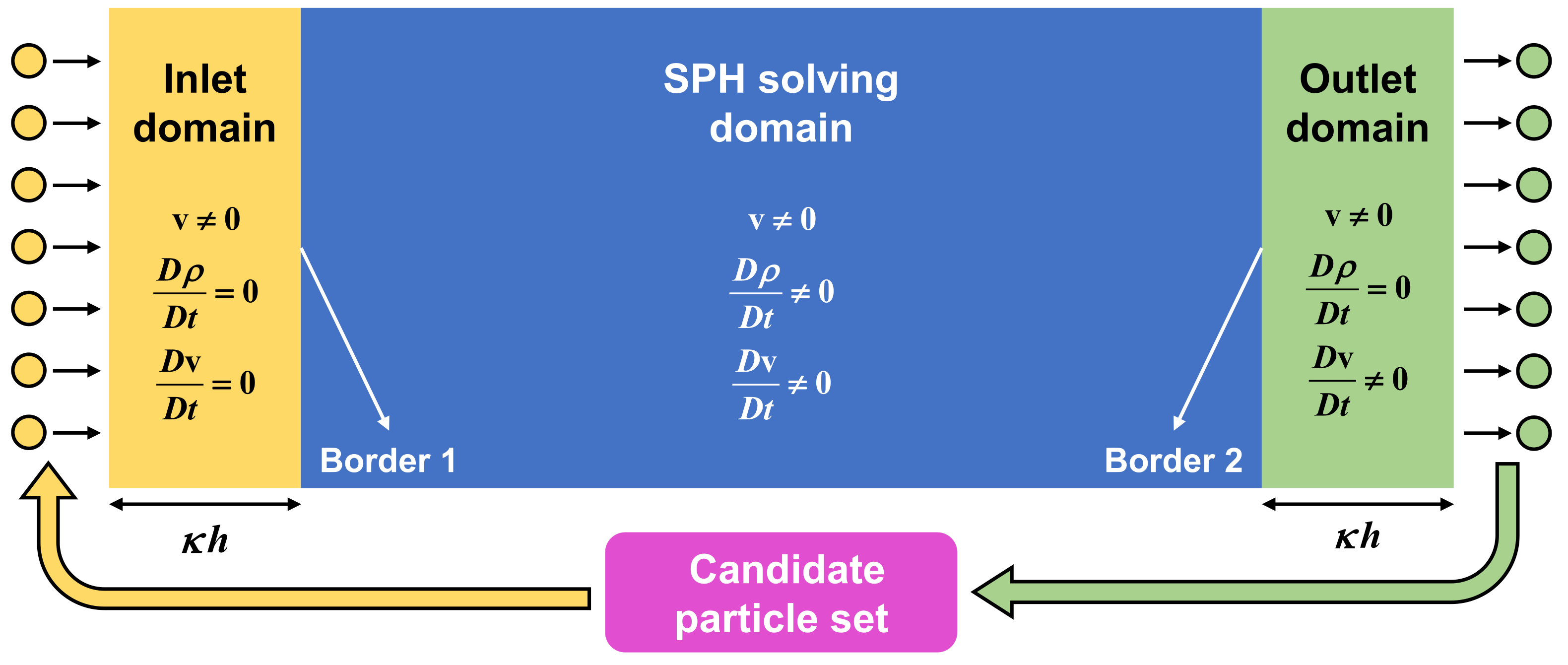
- Lastiwka, M.; Basa, M.; Quinlan, N.J. Permeable and non-reflecting boundary conditions in SPH. Int. J. Numer. Methods Fluids 2009, 61, 709–724. [Google Scholar] [CrossRef] [Green Version]
- Federico, I.; Marrone, S.; Colagrossi, A.; Aristodemo, F.; Antuono, M. Simulating 2D open-channel flows through an SPH model. Eur. J. Mech. B Fluids 2012, 34, 35–46. [Google Scholar] [CrossRef]
- Vacondio, R.; Rogers, B.D.; Stansby, P.K.; Mignosa, P. SPH Modeling of Shallow Flow with Open Boundaries for Practical Flood Simulation. J. Hydraul. Eng. 2012, 138, 530–541. [Google Scholar] [CrossRef]
- Khorasanizade, S.; Sousa, J.M.M. An innovative open boundary treatment for incompressible SPH. Int. J. Numer. Methods Fluids 2016, 80, 161–180. [Google Scholar] [CrossRef]
- Oger, G.; Marrone, S.; Le Touzé, D.; de Leffe, M. SPH accuracy improvement through the combination of a quasi-Lagrangian shifting transport velocity and consistent ALE formalisms. J. Comput. Phys. 2016, 313, 76–98. [Google Scholar] [CrossRef]
- Antuono, M.; Bouscasse, B.; Colagrossi, A.; Marrone, S. A measure of spatial disorder in particle methods. Comput. Phys. Commun. 2014, 185, 2609–2621. [Google Scholar] [CrossRef]
- Xu, R.; Stansby, P.; Laurence, D. Accuracy and stability in incompressible SPH (ISPH) based on the projection method and a new approach. J. Comput. Phys. 2009, 228, 6703–6725. [Google Scholar] [CrossRef]
- Adami, S.; Hu, X.Y.; Adams, N.A. A transport-velocity formulation for smoothed particle hydrodynamics. J. Comput. Phys. 2013, 241, 292–307. [Google Scholar] [CrossRef]
- Mokos, A.; Rogers, B.D.; Stansby, P.K. A multi-phase particle shifting algorithm for SPH simulations of violent hydrodynamics with a large number of particles. J. Hydraul. Res. 2016, 55, 143–162. [Google Scholar] [CrossRef] [Green Version]
- Huang, C.; Zhang, D.H.; Shi, Y.X.; Si, Y.L.; Huang, B. Coupled finite particle method with a modified particle shifting technology. Int. J. Numer. Methods Eng. 2018, 113, 179–207. [Google Scholar] [CrossRef]
- Huang, C.; Long, T.; Li, S.M.; Liu, M.B. A kernel gradient-free SPH method with iterative particle shifting technology for modeling low-Reynolds flows around airfoils. Eng. Anal. Bound. Elem. 2019, 106, 571–587. [Google Scholar] [CrossRef]
- Sun, P.N.; Colagrossi, A.; Marrone, S.; Antuono, M.; Zhang, A.M. A consistent approach to particle shifting in the δ-Plus-SPH model. Comput. Methods Appl. Mech. Eng. 2019, 348, 912–934. [Google Scholar] [CrossRef]
- Wang, P.P.; Meng, Z.F.; Zhang, A.M.; Ming, F.R.; Sun, P.N. Improved particle shifting technology and optimized free-surface detection method for free-surface flows in smoothed particle hydrodynamics. Comput. Methods Appl. Mech. Eng. 2019, 357, 112580. [Google Scholar] [CrossRef]
- Krimi, A.; Jandaghian, M.; Shakibaeinia, A. A WCSPH Particle Shifting Strategy for Simulating Violent Free Surface Flows. Water 2020, 12, 3189. [Google Scholar] [CrossRef]
- Jandaghian, M.; Krimi, A.; Zarrati, A.R.; Shakibaeinia, A. Enhanced weakly-compressible MPS method for violent free-surface flows: Role of particle regularization techniques. J. Comput. Phys. 2021, 434, 110202. [Google Scholar] [CrossRef]
- Jiang, T.; Ren, J.; Yuan, J.; Zhou, W.; Wang, D.S. A least-squares particle model with other techniques for 2D viscoelastic fluid/free surface flow. J. Comput. Phys. 2020, 407, 109255. [Google Scholar] [CrossRef]
- Lyu, H.G.; Sun, P.N. Further enhancement of the particle shifting technique: Towards better volume conservation and particle distribution in SPH simulations of violent free-surface flows. Appl. Math. Model. 2022, 101, 214–238. [Google Scholar] [CrossRef]
- Antuono, M.; Sun, P.N.; Marrone, S.; Colagrossi, A. The δ-ALE-SPH model: An arbitrary Lagrangian-Eulerian framework for the δ-SPH model with particle shifting technique. Comput. Fluids 2021, 216, 104806. [Google Scholar] [CrossRef]
- Liu, M.B.; Liu, G.R. Restoring particle consistency in smoothed particle hydrodynamics. Appl. Numer. Math. 2006, 56, 19–36. [Google Scholar] [CrossRef]
- Wang, P.P.; Zhang, A.M.; Meng, Z.F.; Ming, F.R.; Fang, X.L. A new type of WENO scheme in SPH for compressible flows with discontinuities. Comput. Methods Appl. Mech. Eng. 2021, 381, 113770. [Google Scholar] [CrossRef]
- Sun, P.N.; Colagrossi, A.; Marrone, S.; Antuono, M.; Zhang, A.M. Multi-resolution Delta-plus-SPH with tensile instability control: Towards high Reynolds number flows. Comput. Phys. Commun. 2018, 224, 63–80. [Google Scholar] [CrossRef]
- Antuono, M.; Marrone, S.; Di Mascio, A.; Colagrossi, A. Smoothed particle hydrodynamics method from a large eddy simulation perspective. Generalization to a quasi-Lagrangian model. Phys. Fluids 2021, 33, 015102. [Google Scholar] [CrossRef]
- Moghimi, M.H.; Quinlan, N.J. Application of background pressure with kinematic criterion for free surface extension to suppress non-physical voids in the finite volume particle method. Eng. Anal. Bound. Elem. 2019, 106, 126–138. [Google Scholar] [CrossRef] [Green Version]
- Dalton, G.; Alcorn, R.; Lewis, T. Case study feasibility analysis of the Pelamis wave energy convertor in Ireland, Portugal and North America. Renew. Energy 2010, 35, 443–455. [Google Scholar] [CrossRef]
- Hansen, R.H.; Kramer, M.M.; Vidal, E. Discrete Displacement Hydraulic Power Take-Off System for the Wavestar Wave Energy Converter. Energies 2013, 6, 4001–4044. [Google Scholar] [CrossRef]
- Wen, H.; Ren, B.; Yu, X. An improved SPH model for turbulent hydrodynamics of a 2D oscillating water chamber. Ocean Eng. 2018, 150, 152–166. [Google Scholar] [CrossRef]
- Madhi, F.; Yeung, R.W. On survivability of asymmetric wave-energy converters in extreme waves. Renew. Energy 2018, 119, 891–909. [Google Scholar] [CrossRef]
- Yeylaghi, S.; Moa, B.; Oshkai, P.; Buckham, B.; Crawford, C. ISPH modelling of an oscillating wave surge converter using an OpenMP-based parallel approach. J. Ocean Eng. Mar. Energy 2016, 2, 301–312. [Google Scholar] [CrossRef] [Green Version]
- Zhang, D.H.; Shi, Y.X.; Huang, C.; Si, Y.L.; Huang, B.; Li, W. SPH method with applications of oscillating wave surge converter. Ocean Eng. 2018, 152, 273–285. [Google Scholar] [CrossRef]
- Marrone, S.; Colagrossi, A.; Baudry, V.; Le Touzé, D. Extreme wave impacts on a wave energy converter: Load prediction through a SPH model. Coast. Eng. J. 2019, 61, 63–77. [Google Scholar] [CrossRef]
- Papillon, L.; Costello, R.; Ringwood, J.V. Boundary element and integral methods in potential flow theory: A review with a focus on wave energy applications. J. Ocean Eng. Mar. Energy 2020, 6, 303–337. [Google Scholar] [CrossRef]
- Sirnivas, S.; Yu, Y.H.; Hall, M.; Bosma, B. Coupled Mooring. Analyses for the WEC-Sim Wave Energy Converter Design Tool, Volume 6: Ocean Space Utilization; Ocean Renewable Energy. In Proceedings of the International Conference on Offshore Mechanics and Arctic Engineering, Busan, Korea, 19–24 June 2016. [Google Scholar]
- Liu, Y.C.; Peng, Y.; Wan, D.C. Numerical Investigation on Interaction between a Semi-Submersible Platform and Its Mooring System, Volume 7: Ocean Engineering. In Proceedings of the International Conference on Offshore Mechanics and Arctic Engineering, St. John’s, NL, Canada, 31 May–5 June 2015. [Google Scholar]
- Palm, J.; Eskilsson, C.; Paredes, G.M.; Bergdahl, L. Coupled mooring analysis for floating wave energy converters using CFD: Formulation and validation. Int. J. Mar. Energy 2016, 16, 83–99. [Google Scholar] [CrossRef] [Green Version]
- Wang, J.H.; Zhao, W.W.; Wan, D.C. Development of naoe-FOAM-SJTU solver based on OpenFOAM for marine hydrodynamics. J. Hydrodyn. 2019, 31, 1–20. [Google Scholar] [CrossRef]
- He, J.W.; Wan, D.C.; Hu, Z.Q. CFD Simulations of Helical Strakes Reducing Vortex Induced Motion of a Semi-Submersible, Volume 2: CFD and FSI. In Proceedings of the International Conference on Offshore Mechanics and Arctic Engineering, Madrid, Spain, 17–22 June 2018. [Google Scholar]
- Liu, Y.; Xiao, Q.; Incecik, A.; Peyrard, C.; Wan, D. Establishing a fully coupled CFD analysis tool for floating offshore wind turbines. Renew. Energy 2017, 112, 280–301. [Google Scholar] [CrossRef] [Green Version]
- Liu, Y.; Xiao, Q. Development of a fully coupled aero-hydro-mooring-elastic tool for floating offshore wind turbines. J. Hydrodyn. 2019, 31, 21–33. [Google Scholar] [CrossRef] [Green Version]
- The MoorDyn Solver. Available online: https://github.com/mattEhall/MoorDyn (accessed on 25 November 2021).
- Tasora, A.; Anitescu, M. A matrix-free cone complementarity approach for solving large-scale, nonsmooth, rigid body dynamics. Comput. Methods Appl. Mech. Eng. 2011, 200, 439–453. [Google Scholar] [CrossRef] [Green Version]
- Sherman, M.A.; Seth, A.; Delp, S.L. Simbody: Multibody dynamics for biomedical research. Procedia IUTAM 2011, 2, 241–261. [Google Scholar] [CrossRef] [PubMed] [Green Version]
- Barreiro, A.; Crespo, A.J.C.; Dominguez, J.M.; Garcia-Feal, O.; Zabala, I.; Gomez-Gesteira, M. Quasi-static mooring solver implemented in SPH. J. Ocean Eng. Mar. Energy 2016, 2, 381–396. [Google Scholar] [CrossRef] [Green Version]
- Crespo, A.; Altomare, C.; Domínguez, J.; González-Cao, J.; Gómez-Gesteira, M. Towards simulating floating offshore oscillating water column converters with Smoothed Particle Hydrodynamics. Coast. Eng. 2017, 126, 11–26. [Google Scholar] [CrossRef]
- Domínguez, J.M.; Crespo, A.J.C.; Hall, M.; Altomare, C.; Wu, M.; Stratigaki, V.; Troch, P.; Cappietti, L.; Gómez-Gesteira, M. SPH simulation of floating structures with moorings. Coast. Eng. 2019, 153, 103560. [Google Scholar] [CrossRef]
- Liu, Z.; Wang, Y. Numerical studies of submerged moored box-type floating breakwaters with different shapes of cross-sections using SPH. Coast. Eng. 2020, 158, 103687. [Google Scholar] [CrossRef]
- Liu, Z.; Wang, Y. Numerical investigations and optimizations of typical submerged box-type floating breakwaters using SPH. Ocean Eng. 2020, 209, 107475. [Google Scholar] [CrossRef]
- Ropero-Giralda, P.; Crespo, A.J.C.; Tagliafierro, B.; Altomare, C.; Domínguez, J.M.; Gómez-Gesteira, M.; Viccione, G. Efficiency and survivability analysis of a point-absorber wave energy converter using DualSPHysics. Renew. Energy 2020, 162, 1763–1776. [Google Scholar] [CrossRef]
- Ropero-Giralda, P.; Crespo, A.J.C.; Coe, R.G.; Tagliafierro, B.; Domínguez, J.M.; Bacelli, G.; Gómez-Gesteira, M. Modelling a Heaving Point-Absorber with a Closed-Loop Control System Using the DualSPHysics Code. Energies 2021, 14, 760. [Google Scholar] [CrossRef]
- Quartier, N.; Ropero-Giralda, P.M.; Domínguez, J.;; Stratigaki, V.;; Troch, P. Influence of the Drag Force on the Average Absorbed Power of Heaving Wave Energy Converters Using Smoothed Particle Hydrodynamics. Water 2021, 13, 384. [Google Scholar] [CrossRef]
- Brito, M.; Canelas, R.B.; García-Feal, O.; Domínguez, J.M.; Crespo, A.J.C.; Ferreira, R.M.L.; Neves, M.G.; Teixeira, L. A numerical tool for modelling oscillating wave surge converter with nonlinear mechanical constraints. Renew. Energy 2020, 146, 2024–2043. [Google Scholar] [CrossRef]
- Cui, J.; Chen, X.; Sun, P. Numerical investigation on the hydrodynamic performance of a new designed breakwater using smoothed particle hydrodynamic method. Eng. Anal. Bound. Elem. 2021, 130, 379–403. [Google Scholar] [CrossRef]
- Zhang, C.; Rezavand, M.; Hu, X. A multi-resolution SPH method for fluid-structure interactions. J. Comput. Phys. 2021, 429, 110028. [Google Scholar] [CrossRef]
- Wei, Z.; Edge, B.L.; Dalrymple, R.A.; Hérault, A. Modeling of wave energy converters by GPUSPH and Project Chrono. Ocean Eng. 2019, 183, 332–349. [Google Scholar] [CrossRef]
- Wang, C.; Tay, Z.Y.; Takagi, K.; Utsunomiya, T. Literature Review of Methods for Mitigating Hydroelastic Response of VLFS Under Wave Action. Appl. Mech. Rev. 2010, 63, 030802. [Google Scholar] [CrossRef]
- Ding, J.; Wu, Y.; Xie, Z.; Yang, W.; Wang, S.; Yu, J.; Yu, T. Overview: Research on hydroelastic responses of VLFS in complex environments. Mar. Struct. 2021, 78, 102978. [Google Scholar] [CrossRef]
- Collins, I.; Hossain, M.; Dettmer, W.; Masters, I. Flexible membrane structures for wave energy harvesting: A review of the developments, materials and computational modelling approaches. Renew. Sustain. Energy Rev. 2021, 151, 111478. [Google Scholar] [CrossRef]
- Long, T.; Huang, C.; Hu, D.; Liu, M. Coupling edge-based smoothed finite element method with smoothed particle hydrodynamics for fluid structure interaction problems. Ocean Eng. 2021, 225, 108772. [Google Scholar] [CrossRef]
- Yang, Q.; Jones, V.; McCue, L. Free-surface flow interactions with deformable structures using an SPH–FEM model. Ocean Eng. 2012, 55, 136–147. [Google Scholar] [CrossRef]
- Ming, F.; Zhang, A.; Xue, Y.; Wang, S. Damage characteristics of ship structures subjected to shockwaves of underwater contact explosions. Ocean Eng. 2016, 117, 359–382. [Google Scholar] [CrossRef]
- Long, T.; Hu, D.; Wan, D.; Zhuang, C.; Yang, G. An arbitrary boundary with ghost particles incorporated in coupled FEM–SPH model for FSI problems. J. Comput. Phys. 2017, 350, 166–183. [Google Scholar] [CrossRef]
- Zhang, N.; Yan, S.; Zheng, X.; Ma, Q. A 3D Hybrid Model Coupling SPH and QALE-FEM for Simulating Nonlinear Wave-structure Interaction. Int. J. Offshore Polar Eng. 2020, 30, 11–19. [Google Scholar] [CrossRef]
- Hu, T.; Wang, S.; Zhang, G.; Sun, Z.; Zhou, B. Numerical simulations of sloshing flows with an elastic baffle using a SPH-SPIM coupled method. Appl. Ocean Res. 2019, 93, 101950. [Google Scholar] [CrossRef]
- Zhang, G.; Hu, T.; Sun, Z.; Wang, S.; Shi, S.; Zhang, Z. A δSPH–SPIM coupled method for fluid–structure interaction problems. J. Fluids Struct. 2021, 101, 103210. [Google Scholar] [CrossRef]
- Rao, C.p.; Wan, D.c. Numerical study of the wave-induced slamming force on the elastic plate based on MPS-FEM coupled method. J. Hydrodyn. 2018, 30, 70–78. [Google Scholar] [CrossRef]
- Zheng, H.; Shioya, R. Verifications for Large-Scale Parallel Simulations of 3D Fluid–Structure Interaction Using Moving Particle Simulation (MPS) and Finite Element Method (FEM). Int. J. Comput. Methods 2019, 16, 1840014. [Google Scholar] [CrossRef]
- Zhang, Y.; Wan, D. MPS-FEM Coupled Method for Fluid–Structure Interaction in 3D Dam-Break Flows. Int. J. Comput. Methods 2019, 16, 1846009. [Google Scholar] [CrossRef]
- He, J.; Tofighi, N.; Yildiz, M.; Lei, J.; Suleman, A. A coupled WC-TL SPH method for simulation of hydroelastic problems. Int. J. Comput. Fluid Dyn. 2017, 31, 174–187. [Google Scholar] [CrossRef]
- Sun, P.N.; Le Touzé, D.; Zhang, A.M. Study of a complex fluid-structure dam-breaking benchmark problem using a multi-phase SPH method with APR. Eng. Anal. Bound. Elem. 2019, 104, 240–258. [Google Scholar] [CrossRef]
- Zhan, L.; Peng, C.; Zhang, B.; Wu, W. A stabilized TL–WC SPH approach with GPU acceleration for three-dimensional fluid–structure interaction. J. Fluids Struct. 2019, 86, 329–353. [Google Scholar] [CrossRef]
- Islam, M.R.I.; Peng, C. A Total Lagrangian SPH method for modelling damage and failure in solids. Int. J. Mech. Sci. 2019, 157–158, 498–511. [Google Scholar] [CrossRef] [Green Version]
- Sun, P.N.; Le Touzé, D.; Oger, G.; Zhang, A.M. An accurate FSI-SPH modeling of challenging fluid-structure interaction problems in two and three dimensions. Ocean Eng. 2021, 221, 108552. [Google Scholar] [CrossRef]
- Peng, Y.X.; Zhang, A.M.; Ming, F.R. Numerical simulation of structural damage subjected to the near-field underwater explosion based on SPH and RKPM. Ocean Eng. 2021, 222, 108576. [Google Scholar] [CrossRef]
- Peng, Y.X.; Zhang, A.M.; Wang, S.P. Coupling of WCSPH and RKPM for the simulation of incompressible fluid–structure interactions. J. Fluids Struct. 2021, 102, 103254. [Google Scholar] [CrossRef]
- Ren, B.; Fan, H.; Bergel, G.L.; Regueiro, R.A.; Lai, X.; Li, S. A peridynamics–SPH coupling approach to simulate soil fragmentation induced by shock waves. Comput. Mech. 2015, 55, 287–302. [Google Scholar] [CrossRef]
- Fan, H.; Bergel, G.L.; Li, S. A hybrid peridynamics–SPH simulation of soil fragmentation by blast loads of buried explosive. Int. J. Impact Eng. 2016, 87, 14–27. [Google Scholar] [CrossRef] [Green Version]
- Fan, H.; Li, S. A Peridynamics-SPH modeling and simulation of blast fragmentation of soil under buried explosive loads. Comput. Methods Appl. Mech. Eng. 2017, 318, 349–381. [Google Scholar] [CrossRef]
- Sun, W.K.; Zhang, L.W.; Liew, K. A smoothed particle hydrodynamics–peridynamics coupling strategy for modeling fluid–structure interaction problems. Comput. Methods Appl. Mech. Eng. 2020, 371, 113298. [Google Scholar] [CrossRef]
- O Connor, J.; Rogers, B.D. A fluid–structure interaction model for free-surface flows and flexible structures using smoothed particle hydrodynamics on a GPU. J. Fluids Struct. 2021, 104, 103312. [Google Scholar] [CrossRef]
- Khayyer, A.; Gotoh, H.; Falahaty, H.; Shimizu, Y. An enhanced ISPH–SPH coupled method for simulation of incompressible fluid–elastic structure interactions. Comput. Phys. Commun. 2018, 232, 139–164. [Google Scholar] [CrossRef]
- Khayyer, A.; Tsuruta, N.; Shimizu, Y.; Gotoh, H. Multi-resolution MPS for incompressible fluid-elastic structure interactions in ocean engineering. Appl. Ocean Res. 2019, 82, 397–414. [Google Scholar] [CrossRef]
- Khayyer, A.; Shimizu, Y.; Gotoh, H.; Hattori, S. Multi-resolution ISPH-SPH for accurate and efficient simulation of hydroelastic fluid-structure interactions in ocean engineering. Ocean Eng. 2021, 226, 108652. [Google Scholar] [CrossRef]
- Panciroli, R.; Abrate, S.; Minak, G.; Zucchelli, A. Hydroelasticity in water-entry problems: Comparison between experimental and SPH results. Compos. Struct. 2012, 94, 532–539. [Google Scholar] [CrossRef]
- Khayyer, A.; Shimizu, Y.; Gotoh, H.; Nagashima, K. A coupled incompressible SPH-Hamiltonian SPH solver for hydroelastic FSI corresponding to composite structures. Appl. Math. Model. 2021, 94, 242–271. [Google Scholar] [CrossRef]
- Ji, B.; Luo, X.; Wu, Y.; Peng, X.; Duan, Y. Numerical analysis of unsteady cavitating turbulent flow and shedding horse-shoe vortex structure around a twisted hydrofoil. Int. J. Multiph. Flow 2013, 51, 33–43. [Google Scholar] [CrossRef] [Green Version]
- Luo, X.w.; Ji, B.; Tsujimoto, Y. A review of cavitation in hydraulic machinery. J. Hydrodyn. 2016, 28, 335–358. [Google Scholar] [CrossRef]
- Long, X.; Cheng, H.; Ji, B.; Arndt, R.E.; Peng, X. Large eddy simulation and Euler–Lagrangian coupling investigation of the transient cavitating turbulent flow around a twisted hydrofoil. Int. J. Multiph. Flow 2018, 100, 41–56. [Google Scholar] [CrossRef]
- Cheng, H.; Bai, X.; Long, X.; Ji, B.; Peng, X.; Farhat, M. Large eddy simulation of the tip-leakage cavitating flow with an insight on how cavitation influences vorticity and turbulence. Appl. Math. Model. 2020, 77, 788–809. [Google Scholar] [CrossRef]
- Van Paepegem, W.; Blommaert, C.; De Baere, I.; Degrieck, J.; De Backer, G.; De Rouck, J.; Degroote, J.; Vierendeels, J.; Matthys, S.; Taerwe, L. Slamming wave impact of a composite buoy for wave energy applications: Design and large-scale testing. Polym. Compos. 2011, 32, 700–713. [Google Scholar] [CrossRef]
- Martínez-Ferrer, P.J.; Qian, L.; Causon, D.M.; Mingham, C.G.; Ma, Z. Numerical Simulation of Wave Slamming on a Flap-Type Oscillating Wave Energy Device. Int. J. Offshore Polar Eng. 2018, 28, 65–71. [Google Scholar] [CrossRef]
- Renzi, E.; Wei, Y.; Dias, F. The pressure impulse of wave slamming on an oscillating wave energy converter. J. Fluids Struct. 2018, 82, 258–271. [Google Scholar] [CrossRef] [Green Version]
- Hu, X.Y.; Adams, N.A. A multi-phase SPH method for macroscopic and mesoscopic flows. J. Comput. Phys. 2006, 213, 844–861. [Google Scholar] [CrossRef]
- Grenier, N.; Antuono, M.; Colagrossi, A.; Le Touzé, D.; Alessandrini, B. An Hamiltonian interface SPH formulation for multi-fluid and free surface flows. J. Comput. Phys. 2009, 228, 8380–8393. [Google Scholar] [CrossRef]
- Hammani, I.; Marrone, S.; Colagrossi, A.; Oger, G.; Le Touzé, D. Detailed study on the extension of the δ-SPH model to multi-phase flow. Comput. Methods Appl. Mech. Eng. 2020, 368, 113189. [Google Scholar] [CrossRef]
- Sun, P.N.; Le Touzé, D.; Oger, G.; Zhang, A.M. An accurate SPH Volume Adaptive Scheme for modeling strongly-compressible multiphase flows. Part 1: Numerical scheme and validations with basic 1D and 2D benchmarks. J. Comput. Phys. 2020, 426, 109937. [Google Scholar] [CrossRef]
- Sun, P.N.; Le Touzé, D.; Oger, G.; Zhang, A.M. An accurate SPH Volume Adaptive Scheme for modeling strongly-compressible multiphase flows. Part 2: Extension of the scheme to cylindrical coordinates and simulations of 3D axisymmetric problems with experimental validations. J. Comput. Phys. 2020, 426, 109936. [Google Scholar] [CrossRef]
- Jiang, T.; Li, Y.; Sun, P.N.; Ren, J.L.; Li, Q.; Yuan, J.Y. A corrected WCSPH scheme with improved interface treatments for the viscous/viscoelastic two-phase flows. Comput. Part. Mech. 2021, 8, 1–21. [Google Scholar] [CrossRef]
- Zhu, G.; Graham, D.; Zheng, S.; Hughes, J.; Greaves, D. Hydrodynamics of onshore oscillating water column devices: A numerical study using smoothed particle hydrodynamics. Ocean Eng. 2020, 218, 108226. [Google Scholar] [CrossRef]
- Quartier, N.; Crespo, A.J.C.; Domínguez, J.M.; Stratigaki, V.; Troch, P. Efficient response of an onshore Oscillating Water Column Wave Energy Converter using a one-phase SPH model coupled with a multiphysics library. Appl. Ocean Res. 2021, 115, 102856. [Google Scholar] [CrossRef]
- Sarfaraz, M.; Pak, A. SPH numerical simulation of tsunami wave forces impinged on bridge superstructures. Coast. Eng. 2017, 121, 145–157. [Google Scholar] [CrossRef]
- Barcarolo, D.A.; Le Touzé, D.; Oger, G.; de Vuyst, F. Adaptive particle refinement and derefinement applied to the smoothed particle hydrodynamics method. J. Comput. Phys. 2014, 273, 640–657. [Google Scholar] [CrossRef]
- Chiron, L.; Oger, G.; de Leffe, M.; Le Touzé, D. Analysis and improvements of Adaptive Particle Refinement (APR) through CPU time, accuracy and robustness considerations. J. Comput. Phys. 2018, 354, 552–575. [Google Scholar] [CrossRef]
- Yang, X.; Kong, S.C. Adaptive resolution for multiphase smoothed particle hydrodynamics. Comput. Phys. Commun. 2019, 239, 112–125. [Google Scholar] [CrossRef] [Green Version]
- Yang, X.; Kong, S.C.; Liu, M.; Liu, Q. Smoothed particle hydrodynamics with adaptive spatial resolution (SPH-ASR) for free surface flows. J. Comput. Phys. 2021, 443, 110539. [Google Scholar] [CrossRef]
- Hu, W.; Guo, G.; Hu, X.; Negrut, D.; Xu, Z.; Pan, W. A consistent spatially adaptive smoothed particle hydrodynamics method for fluid–structure interactions. Comput. Methods Appl. Mech. Eng. 2019, 347, 402–424. [Google Scholar] [CrossRef] [Green Version]
- Sun, P.N.; Colagrossi, A.; Marrone, S.; Zhang, A.M. Nonlinear water wave interactions with floating bodies using the δplus-SPH model. In Proceedings of the 32th International Workshop on Water Waves and Floating Bodies (IWWWFB), Dalian, China, 23–26 April 2017. [Google Scholar]
- Gong, K.; Shao, S.; Liu, H.; Wang, B.; Tan, S.K. Two-phase SPH simulation of fluid–structure interactions. J. Fluids Struct. 2016, 65, 155–179. [Google Scholar] [CrossRef] [Green Version]
- Markauskas, D.; Kruggel-Emden, H.; Sivanesapillai, R.; Steeb, H. Comparative study on mesh-based and mesh-less coupled CFD-DEM methods to model particle-laden flow. Powder Technol. 2017, 305, 78–88. [Google Scholar] [CrossRef] [Green Version]
- Markauskas, D.; Kruggel-Emden, H. Coupled DEM-SPH simulations of wet continuous screening. Adv. Powder Technol. 2019, 30, 2997–3009. [Google Scholar] [CrossRef]
- Xu, W.J.; Dong, X.Y.; Ding, W.T. Analysis of fluid-particle interaction in granular materials using coupled SPH-DEM method. Powder Technol. 2019, 353, 459–472. [Google Scholar] [CrossRef]
- Peng, C.; Zhan, L.; Wu, W.; Zhang, B. A fully resolved SPH-DEM method for heterogeneous suspensions with arbitrary particle shape. Powder Technol. 2021, 387, 509–526. [Google Scholar] [CrossRef]
- Ng, K.C.; Alexiadis, A.; Chen, H.; Sheu, T.W.H. Numerical computation of fluid–solid mixture flow using the SPH–VCPM–DEM method. J. Fluids Struct. 2021, 106, 103369. [Google Scholar] [CrossRef]
- Serván-Camas, B.; Cercós-Pita, J.; Colom-Cobb, J.; García-Espinosa, J.; Souto-Iglesias, A. Time domain simulation of coupled sloshing–seakeeping problems by SPH–FEM coupling. Ocean Eng. 2016, 123, 383–396. [Google Scholar] [CrossRef] [Green Version]
- Marrone, S.; Di Mascio, A.; Le Touzé, D. Coupling of Smoothed Particle Hydrodynamics with Finite Volume method for free-surface flows. J. Comput. Phys. 2016, 310, 161–180. [Google Scholar] [CrossRef]
- Chiron, L.; Marrone, S.; Di Mascio, A.; Le Touzé, D. Coupled SPH–FV method with net vorticity and mass transfer. J. Comput. Phys. 2018, 364, 111–136. [Google Scholar] [CrossRef]
- Bai, B.; Rao, D.; Xu, T.; Chen, P. SPH-FDM boundary for the analysis of thermal process in homogeneous media with a discontinuous interface. Int. J. Heat Mass Transf. 2018, 117, 517–526. [Google Scholar] [CrossRef]
- Huang, C.; Long, T.; Liu, M.B. Coupling finite difference method with finite particle method for modeling viscous incompressible flows. Int. J. Numer. Methods Fluids 2019, 90, 564–583. [Google Scholar] [CrossRef]
- Di Mascio, A.; Marrone, S.; Colagrossi, A.; Chiron, L.; Le Touzé, D. SPH–FV coupling algorithm for solving multi-scale three-dimensional free-surface flows. Appl. Ocean Res. 2021, 115, 102846. [Google Scholar] [CrossRef]
- Domínguez, J.M.; Crespo, A.J.C.; Gómez-Gesteira, M. Optimization strategies for CPU and GPU implementations of a smoothed particle hydrodynamics method. Comput. Phys. Commun. 2013, 184, 617–627. [Google Scholar] [CrossRef]
- Luo, M.; Koh, C. Shared-Memory parallelization of consistent particle method for violent wave impact problems. Appl. Ocean Res. 2017, 69, 87–99. [Google Scholar] [CrossRef] [Green Version]
- Wu, Y.; Tian, L.; Rubinato, M.; Gu, S.; Yu, T.; Xu, Z.; Cao, P.; Wang, X.; Zhao, Q. A New Parallel Framework of SPH-SWE for Dam Break Simulation Based on OpenMP. Water 2020, 12, 1395. [Google Scholar] [CrossRef]
- Cui, X.; Habashi, W.G.; Casseau, V. MPI Parallelisation of 3D Multiphase Smoothed Particle Hydrodynamics. Int. J. Comput. Fluid Dyn. 2020, 34, 610–621. [Google Scholar] [CrossRef]
- Olivier, S.L.; Prins, J.F. Comparison of OpenMP 3.0 and Other Task Parallel Frameworks on Unbalanced Task Graphs. Int. J. Parallel Program. 2010, 38, 341–360. [Google Scholar] [CrossRef] [Green Version]
- Oger, G.; Le Touzé, D.; Guibert, D.; de Leffe, M.; Biddiscombe, J.; Soumagne, J.; Piccinali, J.G. On distributed memory MPI-based parallelization of SPH codes in massive HPC context. Comput. Phys. Commun. 2016, 200, 1–14. [Google Scholar] [CrossRef]
- Yang, E.; Bui, H.H.; De Sterck, H.; Nguyen, G.D.; Bouazza, A. A scalable parallel computing SPH framework for predictions of geophysical granular flows. Comput. Geotech. 2020, 121, 103474. [Google Scholar] [CrossRef]
- Harada, T.; Koshizuka, S.; Kawaguchi, Y. Smotthed Particle Hydrodynamics on GPUs. In Proceedings of the Computer Graphics International 2007, Petropolis, Brazil, 30 May–2 June 2007. [Google Scholar]
- Crespo, A.C.; Dominguez, J.M.; Barreiro, A.; Gómez-Gesteira, M.; Rogers, B.D. GPUs, a New Tool of Acceleration in CFD: Efficiency and Reliability on Smoothed Particle Hydrodynamics Methods. PLoS ONE 2011, 6, e20685. [Google Scholar] [CrossRef]
- Hérault, A.; Bilotta, G.; Dalrymple, R.A. SPH on GPU with CUDA. J. Hydraul. Res. 2010, 48, 74–79. [Google Scholar] [CrossRef]
- Cercos-Pita, J.L. AQUAgpusph, a new free 3D SPH solver accelerated with OpenCL. Comput. Phys. Commun. 2015, 192, 295–312. [Google Scholar] [CrossRef]
- Ramachandran, P.; Bhosale, A.; Puri, K.; Negi, P.; Muta, A.; Dinesh, A.; Menon, D.; Govind, R.; Sanka, S.; Sebastian, A.S.; et al. PySPH: A Python-based Framework for Smoothed Particle Hydrodynamics. ACM Trans. Math. Softw. 2021, 47. [Google Scholar] [CrossRef]
- Domínguez, J.M.; Crespo, A.J.C.; Valdez-Balderas, D.; Rogers, B.D.; Gómez-Gesteira, M. New multi-GPU implementation for smoothed particle hydrodynamics on heterogeneous clusters. Comput. Phys. Commun. 2013, 184, 1848–1860. [Google Scholar] [CrossRef]
- Valdez-Balderas, D.; Domínguez, J.M.; Rogers, B.D.; Crespo, A.J.C. Towards accelerating smoothed particle hydrodynamics simulations for free-surface flows on multi-GPU clusters. J. Parallel Distrib. Comput. 2013, 73, 1483–1493. [Google Scholar] [CrossRef] [Green Version]
- Ji, Z.; Xu, F.; Takahashi, A.; Sun, Y. Large scale water entry simulation with smoothed particle hydrodynamics on single- and multi-GPU systems. Comput. Phys. Commun. 2016, 209, 1–12. [Google Scholar] [CrossRef]
- Morikawa, D.; Senadheera, H.; Asai, M. Explicit incompressible smoothed particle hydrodynamics in a multi-GPU environment for large-scale simulations. Comput. Part. Mech. 2021, 8, 493–510. [Google Scholar] [CrossRef]


| Item | DualSPHysics | SPHinXsys |
|---|---|---|
| Fluid solver | -SPH [107] | Riemann-SPH [112] |
| Structure solver | mDBC [123] | Fixed ghost particle [121] |
| Mooring dynamics | MoorDyn [182] | Not yet officially provided |
| Multibody dynamics | Project Chrono [183] | Simbody [184] |
| Framework | Type | Superiority | Limitation |
|---|---|---|---|
| OpenMP | SMSs | Easy to code | Speedup is limited |
| TBB | SMSs | Better balance for workload | Need to reconstruct codes |
| GPU | SMSs | The fastest framework of SMSs | Capacity is limited |
| MPI | DMSs | Applicable to large-scale problems | Hard to balance workload |
Publisher’s Note: MDPI stays neutral with regard to jurisdictional claims in published maps and institutional affiliations. |
© 2022 by the authors. Licensee MDPI, Basel, Switzerland. This article is an open access article distributed under the terms and conditions of the Creative Commons Attribution (CC BY) license (https://creativecommons.org/licenses/by/4.0/).
Share and Cite
Lyu, H.-G.; Sun, P.-N.; Huang, X.-T.; Zhong, S.-Y.; Peng, Y.-X.; Jiang, T.; Ji, C.-N. A Review of SPH Techniques for Hydrodynamic Simulations of Ocean Energy Devices. Energies 2022, 15, 502. https://doi.org/10.3390/en15020502
Lyu H-G, Sun P-N, Huang X-T, Zhong S-Y, Peng Y-X, Jiang T, Ji C-N. A Review of SPH Techniques for Hydrodynamic Simulations of Ocean Energy Devices. Energies. 2022; 15(2):502. https://doi.org/10.3390/en15020502
Chicago/Turabian StyleLyu, Hong-Guan, Peng-Nan Sun, Xiao-Ting Huang, Shi-Yun Zhong, Yu-Xiang Peng, Tao Jiang, and Chun-Ning Ji. 2022. "A Review of SPH Techniques for Hydrodynamic Simulations of Ocean Energy Devices" Energies 15, no. 2: 502. https://doi.org/10.3390/en15020502
APA StyleLyu, H.-G., Sun, P.-N., Huang, X.-T., Zhong, S.-Y., Peng, Y.-X., Jiang, T., & Ji, C.-N. (2022). A Review of SPH Techniques for Hydrodynamic Simulations of Ocean Energy Devices. Energies, 15(2), 502. https://doi.org/10.3390/en15020502