Abstract
This paper presents an accurate quasi-analytical approximation of frequency-dependent ac resistance of single rectangular conductors. In this work, first, a two-dimensional analytical ac resistance of rectangular conductors is derived. Unlike circular conductors, where current density distributes evenly in each layer of the conductor’s cross-section, the edge effect is involved for rectangular conductors. Due to the edge effect, one cannot define an accurate boundary condition for solving the two-dimensional partial differential equation of magnetic field or current density of rectangular conductors. Hence, the calculated two-dimensional analytical current density result is not accurate and is modified and fitted on FEM simulation, taking the conductor’s thickness into account using the least-square problem to improve its accuracy. Unlike numerical approaches, the proposed method yields an easy-to-use formula applicable to industrial applications in different fields. Contrary to the one-dimensional approach, which is only valid for very thin rectangular conductors, this method takes edge effect into account and can be used for any thickness (from square to very thin rectangular conductors). The proposed method can be used in applications where an accurate ac resistance of rectangular conductors over a wide frequency range is required, such as white-box modeling of power transformers and interpreting its frequency response analysis (FRA), and calculating the resistance of electric machine winding, busbars, and printed circuit board traces.
1. Introduction
Power transformers are valuable assets in a power system which require accurate modeling for their design, monitoring, diagnosis, and maintenance. Frequency response analysis (FRA) is a well-known technique which has been used for these purposes in recent years [1,2,3,4,5,6]. Availability of a transformer model has advantages such as assisting in the interpretation of FRA results [1,2,7], appropriate geometry and material selection at the design stage [8], partial discharge (PD) localization [9,10,11,12], and incorporation in electromagnetic transient (EMT)-type software for transient simulation [13]. Among the types of models developed for a transformer, the so-called white-box model is proven to be a technique for accurate modeling of the internal behaviour of power transformers [14,15]. The resistive loss, which mainly occurs in the winding conductors, and its frequency-dependence (due to the skin and proximity effects), is one of the inputs required for any white box model. The skin effect is the effect of magnetic field of an isolated conductor on itself and is the focus of this manuscript, whereas the proximity effect is the effect of nearby conductors on a conductor’s current distribution. The skin effect pushes the current distribution outwards, towards the surface of a conductor at higher frequencies. It results in higher resistance and increased loss as frequency increases.
In recent years, the frequency-dependent modeling of the resistance of rectangular conductors, where the edge effect is important, has received more attention in electromagnetic transient analysis. The tendency toward electric vehicles and electric drives with high-frequency switching devices requires higher power efficiency and better speed control [16,17,18,19]. The emergence of power electronic converters for interfacing storage batteries, solar panels, etc., results in high-frequency components in transformer voltage and current. This creates higher power losses and hence increased heating and thermal aging of insulation [20]. In power systems, fast transient (up to 3 MHz) and very fast transient (up to 50 MHz) [21] can produce large transient overvoltages, and damage components’ insulation [8]. To appropriately study the effect of these transient phenomena and make a better design, it is required to have an accurate frequency-dependent resistance model of different conductor cross sections, such as rectangular cross section conductors.
The one-dimensional analytical formulation of ac resistance has been developed for very thin rectangular conductors [22,23] and has been employed for transformer [24,25,26,27] and electric machines [28,29] modeling. However, the one-dimensional approach cannot be used for thick rectangular conductors because the magnetic field of such conductors distributes in two dimensions. Hence, a more general formulation for ac resistance of rectangular conductors of any thickness is required. Ametani et al. [30,31,32] derived a general internal impedance approximation for conductors of any cross section from Schelkunoff’s accurate approach for cylindrical conductors [33], and compared it with IEC’s formula for circular conductors [34] for frequencies up to 10 kHz [32]. Riba [35] showed that the IEC formula is only valid for low frequencies. Ametani’s approach has not been verified for rectangular conductors. Nonetheless, it has been used in the literature for applications such as white-box modeling of power transformers with rectangular conductors [11,14,15,21,36]. While it is not easy to define an accurate boundary condition for nonmagnetic rectangular conductors, two different boundary condition definitions are found in the literature [22,23] for two-dimensional analytical calculations of thick rectangular conductors. Experiment shows that both of these two-dimensional analytical approaches are not accurate for nonmagnetic conductors [23]. The well-known ac resistance calculation of circular conductors [23] has been considered for rectangular cross section conductors [1,37,38]. Even though the circular conductor approach gives a good approximation for a square conductor, it is not valid for rectangular (non-square) conductors. There are also numerical approaches [18,39,40,41,42] and conformal mapping solutions [43,44] for calculating ac resistance of rectangular conductors which are not easy to use for engineering applications. The problem has been defined in [45] without proposing any solution, and this paper is a continuation of this work.
This paper proposes an accurate quasi-analytical approximation for the ac resistance of a single rectangular conductor using FEM simulation and a modified two-dimensional analytical calculation. It takes into account the skin effect, the edge effect, and the thickness of rectangular conductors. As the two-dimensional analytical approach is not accurate for nonmagnetic conductors [23], this paper combines it with FEM simulation results using a least-square approach to calculate the ac resistance of rectangular conductors accurately. The proposed approach in this manuscript addresses all the shortcomings of other approaches discussed earlier, by
- Recalculating the two-dimensional analytical ac resistance of single rectangular conductors.
- Reducing the inaccuracy of two-dimensional analytical methods.
- Being simple for engineering applications.
- Being applicable to any rectangular thickness (from square to very thin conductors).
The organization of this paper is as follows. In Section 2, different analytical approximations and FEM simulation for calculating ac resistance are reviewed briefly. It is shown that the two-dimensional analytical method in earlier literature [22] is in error, and a correction is provided in Appendix A. The ac resistance results of different approaches for a circular conductor and different rectangular conductor configurations are provided and discussed in Section 3. A proposed quasi-analytical method is explained in detail in Section 4 to increase the accuracy of ac resistance calculations of 2D analytical approach. Section 5 shows a time-domain simulation to clarify the impact of accurate resistance calculation on damping.
2. Ac Resistance of an Isolated Conductor
There are various analytical approximations for ac resistance of a single isolated rectangular conductor. These approximations, along with the proposed method, are reviewed in this section, and the results are compared with those obtained using FEM simulation in Section 3.
2.1. Circular Conductor
Under the quasi-static assumption, which neglects the displacement current, the ac resistance of a circular conductor of radius , conductivity , and permeability is given by [22,23]
where
The coefficient is the skin depth of the conductor at the frequency of interest. Functions and are the zeroth- and first-order modified Bessel function of the first kind, respectively.
2.2. Ametani’s Approach
Ametani and Fuse proposed a general internal impedance approximation for conductors of any cross section, and calculated the ac resistance as [30,31]
where
In Equation (2), , S, l, and are the conductivity, cross-sectional area, circumferential length (i.e., the perimeter of the conductor), and the permeability of the conductor, respectively. This approach has been used in a wide variety of applications, such as white-box modeling of transformers with rectangular conductors (e.g., see [11,14,15,21,36]).
2.3. One-Dimensional Calculation
Consider a very thin, infinitely long rectangular conductor with dimensions and () [22], as shown in Figure 1. For a general time-harmonic problem with an electric current flowing in the conductor in the z direction, the magnetic field intensity will be in the y direction, and the ac resistance has been calculated as [22,23]
which is further simplified in [22] as
and has been used in many applications, such as transformers [25,26,27] and electrical machines modeling [28,29].
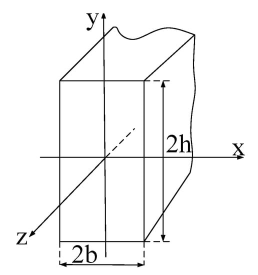
Figure 1.
Schematic of an infinitely long rectangular conductor [22].
2.4. Two-Dimensional Calculation
For a thick rectangular conductor carrying current in the z direction, the magnetic field intensity exists in the x and y directions. As a consequence, the one-dimensional approach is not accurate enough. By combining Maxwell’s equations, a 2D diffusion equation for the z component of the magnetic vector potential A was obtained [23]:
which can also be written in terms of the z component of the current density J [22] as
where . The main concern and difficulty in solving diffusion Equations (4) and (5) is defining accurate boundary conditions. Two main boundary conditions can be found in the literature. In the first approach, which is more suitable for magnetic conductors [23], the surface of the conductor has been considered as a magnetic flux line in which everywhere on the surface of the conductor [23], such that
and current density is given by [23]
In the case of circular conductors and very thin rectangular conductors with constant electric field on their surfaces, the ac resistance is defined as the ratio of surface electric field to the current flowing in the conductor [23]. Knowing that , we used the surface impedance definition for thick rectangular conductors as
In the second approach, a constant and unknown current density, , is considered on the outer boundary of the conductor [22]:
Reference [22] uses the boundary condition Equation (9), but there are some errors in the final result that cause inaccuracies at high frequencies. This is corrected in Appendix A.
According to [23], the results from these two boundary assumptions, Equations (6) and (9), are inconsistent unless , and one should choose one of these two boundary conditions. However, the author of [23] did not calculate ac resistance, and did not prove this claim. The resistance calculation using the surface impedance approach in Equation (8) gives different values for other x and y points as is not unique on the boundary. However, when and are used, the ac resistance of both of these two boundary conditions are exactly the same. For demonstration, a rectangular conductor is considered with conductivity (S/m), and three different dimensions mm, and mm. The ac resistance using both these 2D approaches is compared in Figure 2, and are exactly the same for different dimensions. Moreover, the approach of Equation (8) is easier to work with for optimization purposes and will be used henceforth as the preferred 2D approach.
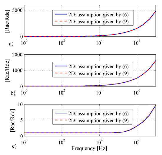
Figure 2.
Ac resistance calculation using 2D analytical approaches for and (a) , (b) , (c) .
2.5. Finite Element Method (FEM) Approach
For a general time-harmonic problem, Maxwell’s equations for an infinitely long conductor with current in the z direction can be written as
where H, E, B, and are magnetic field intensity, electric field intensity, magnetic flux density, and total current density, respectively. The current density is defined as
where , , and are conduction, displacement, and source or external current densities, respectively, and are defined [46] by
and is induced current density. Electric field intensity is composed of two parts [47], given by
where the first part is the Coulomb electric field, defined as , where V is the scalar potential. As the net charge is zero, is equal to zero. The second part is the Faraday electric field, defined as , which is the magnetically induced electric field, and A is the magnetic vector potential. Thus, E can be written as
Under quasi-static approximation, which neglects displacement current, , and knowing that , combining Equations (10)–(17) yields [47]
In this paper, Equation (18) is solved in the two-dimensional (2D) domain using FEM in the frequency range of interest. A Dirichlet boundary condition of is applied to far-enough outer boundaries of the study area.
After solving Equation (18), the r.m.s. value I, the per unit length (p.u.l.) ohmic loss P, and the ac resistance are calculated using
3. Results of ac Resistance Calculation
3.1. Circular Conductor
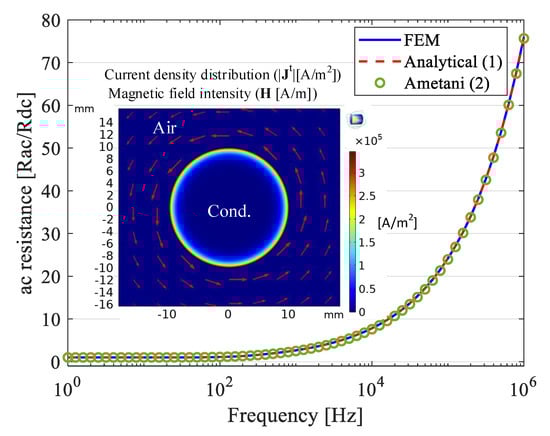
Consider a solid, round conductor with a diameter of and conductivity of carrying current in the frequency range of –. The ac resistance of this conductor calculated using FEM, exact analytical formula, Equation (1) [23], and Ametani’s approach, Equation (2) [30,31], are shown in Figure 3 in which all the results exactly match with each other. Furthermore, the magnitude of current density distribution () at the cross section of the conductor and magnetic field intensity (red arrows) at calculated using FEM are also shown in Figure 3. As shown in Figure 3, due to the skin effect, the current at higher frequencies distributes mostly along the conductor’s outer boundary, consequently results in a smaller effective cross section, and in turn, a higher ac resistance at higher frequencies. Figure 3 verifies that all three approaches accurately calculate ac resistance of circular conductors.
The CPU time requirement and percentage error for various FEM mesh size at are shown in Figure 4. As the error is almost zero for a mesh size less than ten times the skin depth of the conductor (), a mesh size equal to is selected for the rest of the paper. For the case of computationally expensive simulations, such as transformer winding with a number of conductors, it is more suitable to use a fine mesh for the skin depth area and a coarse mesh for the rest of the conductor to increase the efficiency of the computation. For example, by using a mesh size equal to for the skin depth area and for the rest of the conductor, the CPU time decreases from 365 to 12 s, achieving almost the same level of accuracy.
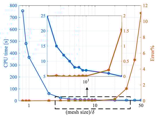
Figure 4.
Effect of FEM mesh size on CPU time and error of resistance calculation of the circular conductor at MHz.
3.2. Foil Type Transformer
A very thin rectangular conductor of LV side of a foil-type transformer with dimensions , (), and conductivity is considered [20]. The ac resistance of the conductor is calculated using 1D analytical Equation (3), 2D analytical Equation (8), Ametani Equation (2), and FEM. As can be seen from Figure 5, the four approaches have identical results. Moreover, the magnitude of current density distribution at the cross section of the conductor, and magnetic field intensity H, calculated using FEM at 10 kHz, are shown in Figure 5. As the conductor is very thin, its width () is smaller than skin depth up to almost , and as a consequence, the current density distributes evenly at the cross section of the conductor. This means no change to the effective cross section of the conductor [48]; hence, the ac resistance eventually equals the dc resistance up to . Due to the thinness of the conductor and, hence, uniform current distribution and magnetic field H only along the y (vertical) axis, the analytical 1D calculation yields the same result as the analytical 2D and FEM.
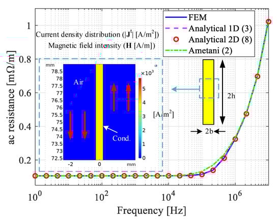
Figure 5.
Ac resistance of the conductor of LV side of the foil type transformer with dimensions mm, mm () [20] at 1–10 MHz, and magnitude of current density distribution, , at the cross section of the conductor and magnetic field intensity, H (red arrows), at .
3.3. Square Conductor
A square conductor with dimension and conductivity is considered [40]. The ac resistance is calculated using 1D analytical Equation (3), 2D analytical Equation (8), Ametani Equation (2), and FEM. The results are compared with published measurement [40], as shown in Figure 6. The magnitude of current density distribution, , at the cross section of the conductor and magnetic field intensity (red arrows), H, are also shown in Figure 6 at 10 kHz. Unlike the very thin rectangular conductor, which has magnetic field intensity in only one direction (i.e., y direction), both x and y components of the magnetic field intensity exist in the square conductor, which must be considered in the calculations. As for square conductors, the assumption of is not valid anymore for 1D calculation. Thus, the 1D approach, Equation (3), is not accurate. The FEM simulation results accurately match with the measurements. The 2D analytical calculation is also accurate, with some errors.
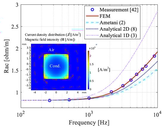
Figure 6.
Ac resistance calculation of a square conductor with dimension mm, conductivity at the frequency range of 1 Hz–10 kHz, and current density distribution, (), at the cross section of the conductor and magnetic field intensity, H (red arrows), at .
Ametani’s approach, Equation (2), is derived from analytical calculations of cylindrical conductors [30,31,33], and it accurately calculates ac resistance of circular conductors (see Figure 3). However, when it comes to rectangular or square conductors, according to Figure 6, more current distributes at the edges of the conductor at higher frequencies. As a consequence, this would produce more resistive loss base on Equation (20), and in turn, higher ac resistance. As Equation (2) does not take the edge effect into account in ac resistance calculation, Ametani’s approach is not very accurate for rectangular conductors.
3.4. Effect of Thickness on Accuracy
The rectangular conductor of Section 3.2 with constant height mm, and variable width between 1–500 mm is considered here. The results of Section 3.3 indicate that the FEM results most accurately match the experimental results, and hence it is used as a template for the discussion in this section. Figure 7 shows the ac resistance for the different approaches versus at 1 MHz. As can be seen, the 1D analytical approach is accurate for , which corresponds to a very thin conductor (). Ametani and the 2D approaches agree well over almost the full range. However, as they do not consider the boundary current distribution for thicker rectangular conductors accurately, they diverge from the FEM result for small ratios. The maximum error is about , which occurs for . However, there is generally good agreement at higher ratios, where the conductor is thin.
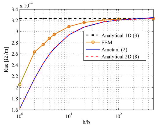
Figure 7.
Ac resistance versus thickness () for constant h and variable b at 1 MHz.
4. Proposed Quasi-Analytical Method for Accurate Calculation of for Rectangular Conductors
This section presents a new quasi-analytical calculation method, which modifies the 2D analytical method to give improved ac resistance values for rectangular conductors when compared with Ametani’s approach or the 2D approaches in [22,23]. The main problem of 2D analytical calculation of thick rectangular conductors is the lack of accurate boundary conditions. To demonstrate this issue, the ac resistance of very thin rectangular conductors with conductivity , mm, and different values ranging from is calculated using FEM and shown in Figure 8. The results show that is a function of the conductor width to skin depth ratio (). However, there is a different scenario for thick conductors. Figure 9a shows a plot of the ac resistance as a function of frequency and Figure 9b shows how varies with conductor width to skin depth ratio for different ratios ranging from 1 to 10. According to Figure 9b, the ac resistance is a function of both and . This observation suggests a way to modify the analytical formula by using the FEM results as follows.
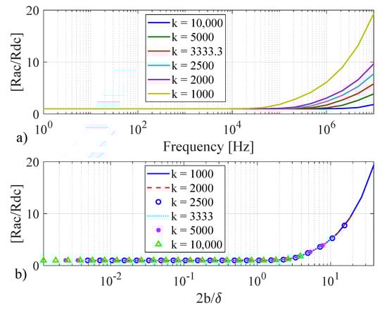
Figure 8.
Ac resistance calculation using FEM of very thin rectangular conductors versus (a) frequency, and (b) , for different dimensions: , mm, and ( 1000:10,000).
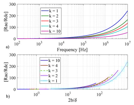
Figure 9.
Ac resistance calculation using FEM of thick rectangular conductors versus (a) frequency, and (b) , for different dimensions: , mm and ().
Based on [19], each ac resistance curve can be defined as two linear functions of k and a, one for and the other one for .
where , , and are unknown. The first part of Equation (23), (i.e., ), shows that when the conductor is sufficiently thin (i.e., ) or the current distributes evenly across the cross section (i.e., ), the two-dimensional analytical calculation is accurate. Moreover, for thicker section, when the width is much greater than skin depth (i.e., ), Equation (22) can be modified and written as a linear combination of and . In this formula, the relative combinations of and are a function of the ratio or k through the multiplying factors () and (). The unknown coefficients , , , and are calculated by solving a least-square problem [49]. , , , and are selected so that Equation (23) fits the FEM-generated data (that in Figure 9) by solving a least-square problem.
Doing so yields the unknown coefficients , , , and as , , , and , based on the conductors in Figure 9. Although shown for a material of , the discussion below shows that the same coefficients work well with other materials also. To analyze the validity of the calculated coefficients for other conductors, three different cases with different dimensions and materials are studied, as follows:
- Case 1: mm, , and S/m.
- Case 2: mm, , and S/m.
- Case 3: mm, , and [40].
The ac resistance of all these three cases are calculated using FEM, the proposed method Equation (23) and the 2D analytical, and the results are shown in Figure 10. According to this figure, the proposed method is very accurate for different thicknesses and materials. The above results show that the formula in Equation (23) can be used to calculate ac resistance for arbitrary conductors without using further computationally-expensive FEM analysis.
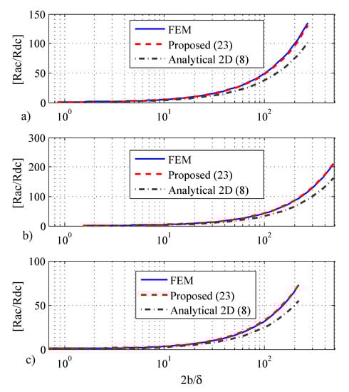
Figure 10.
Ac resistance calculation using FEM, the proposed method Equation (23), and 2D analytical of three different rectangular conductors: (a) mm, , and ; (b) mm, , and S/m; (c) mm, , and conductivity .
5. Transient Simulation
The accurate ac resistance formula Equation (23) is used in this section to show its usefulness in the transient simulation. The square conductor studied in Section 3.3 with 100 m length is considered in a transient study shown in Figure 11 to investigate the effect of different ac resistance calculations on transient simulation. A per-unit Gaussian waveform voltage source with a 10 MHz maximum frequency is considered at the sending end of the conductor with and grounded receiving end. We solved Telegrapher’s equations [50] for calculating currents at both ends of the conductor in which p.u.l. parameters of the conductor are required. The p.u.l. conductance G is considered as zero, inductance L and capacitance C are calculated using magnetostatic and electrostatic [14,45], respectively, and the frequency-dependent is calculated using analytical 1D Equation (3), analytical 2D Equation (8), Ametani (2), FEM, and the proposed method Equation (23). The FEM-based tabulated results are also used as a template for comparison. In this simulation, C and L are calculated as nF/m and nH/m, respectively (see [45] for more discussion).
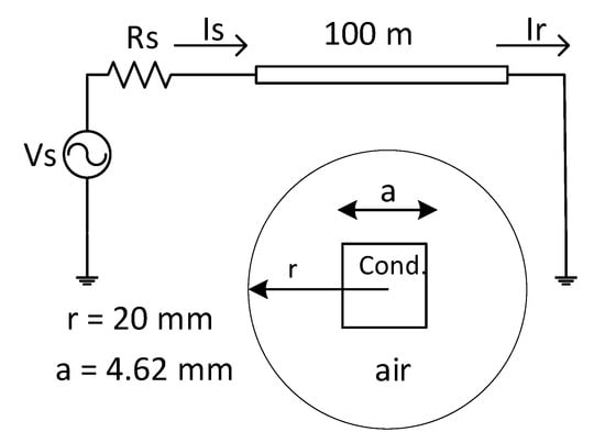
Figure 11.
Square conductor with m, side mm.
The propagation function is defined as [50]
where
In Equation (24), is attenuation constant, and is phase constant. Figure 12 shows the effect of different R calculations on the attenuation constant . Once again, attenuation constant calculated using the proposed approach matches the best with the FEM template results amongst all the approaches. The time-domain results are calculated by applying a frequency-dependent finite difference time-domain (FDTD) analysis [51]. Figure 13 shows the receiving end current in the time domain. Considering a zoomed view around 50 s shown in Figure 13b, the one-dimensional approach of Equation (3) has damped the most among all other approaches and that is due to its largest resistance (see Figure 6), and consequently, the highest attenuation constant (see Figure 12). The envelope of the peak values of the receiving end current is shown in Figure 14.
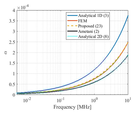
Figure 12.
Attenuation constant of the square conductor.
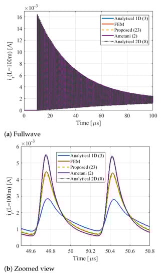
Figure 13.
Receiving end current of the square conductor of Figure 11 due to a Gaussian waveform as the excitation voltage Vs for a time window of (a) 0–100 µs; (b) zoomed view around 50 µs.
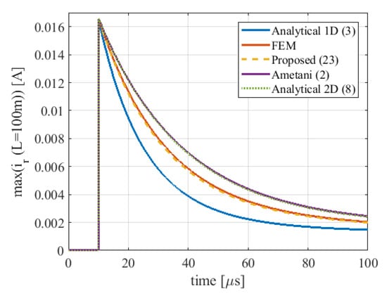
Figure 14.
Envelope of peak values of Figure 13a.
The transient simulation results show that the proposed approach of Equation (23) is very accurate and has almost the same results as FEM, whereas the analytical 2D Equation (8) and Ametani’s Equation (2) approaches are not very accurate. According to Figure 6 and Figure 12, Figure 13 and Figure 14, the higher the R, the larger the , and the better the damping effect. Exact transformer resistance calculation, and, in turn, damping effect calculation, is very important in the determination of the amplitude of resonant waves [8] and transient overvoltage calculations.
6. Conclusions
Different analytical approximation of ac resistance of single rectangular conductors were considered from literature, and their results were compared with those obtained by FEM simulation. It was shown that the one-dimensional analytical calculation was only valid for very thin rectangular conductors, and the two-dimensional analytical and Ametani’s calculations were not accurate for thick rectangular conductors. This is attributed to the fact that due to the edge effect, the distribution of current in the cross section is not calculated accurately in these three formulations. It was shown that the ac resistance of thick rectangular conductors is also a function of conductor thickness, unlike very thin rectangular conductors. In this paper, a new quasi-analytical method was proposed which modeled the analytical 2D method by using a least-square fit, to fit its parameters so that the results accurately matched FEM results. Different conductor thicknesses were used to infer the proposed method. It was shown that the proposed method is very accurate for a variety of conductor dimensions. The proposed model can be used for frequency-dependent resistance modeling of rectangular conductors. The proposed method is computationally efficient and, at the same time, is accurate. Regarding the future work, the effect of proximity on the resistance of rectangular conductors will be formulated and verified. Experimental verification will also be investigated to assess the accuracy of the developed formulations.
Author Contributions
Conceptualization, B.T., A.A., A.M.G. and B.K.; methodology, B.T., A.A., A.M.G. and B.K.; software, B.T.; validation, B.T., A.A., A.M.G. and B.K.; formal analysis, B.T., A.A., A.M.G. and B.K.; investigation, B.T., A.A., A.M.G. and B.K.; resources, A.M.G. and B.K.; data curation, B.T.; writing—original draft preparation, B.T.; writing—review and editing, B.T., A.A., A.M.G. and B.K.; visualization, B.T.; supervision, A.A., A.M.G. and B.K.; project administration, A.M.G. and B.K.; funding acquisition, A.M.G. and B.K. All authors have read and agreed to the published version of the manuscript.
Funding
This research was funded by Natural Sciences and Engineering Research Council of Canada (NSERC).
Institutional Review Board Statement
Not applicable.
Informed Consent Statement
Not applicable.
Data Availability Statement
The data presented in this study are available on request.
Conflicts of Interest
The authors declare no conflict of interest.
Appendix A. Two-Dimensional Analytical Calculations of The Ac Resistance of Rectangular Conductors
Appendix A.1. Calculation of Current Density Distribution
In this section, the analytical derivation of the two dimensional diffusion Equation (A1) with the boundary condition Equation (A2) is provided,
The general answer can be splitted as [52],
Each of these two equations, Equations (A4) and (A5), should be separately solved using equivalent boundary conditions, then combined with Equation (A3) to obtain the final answer. For , it is common to have the separation of variable as [52],
By combining Equations (A4) and (A6), and removing x and y in the functions X and Y for ease in writing, it gives
From boundary conditions, , hence and the new is
From the boundary condition Equation (A4)
where the expression is the Fourier cosine coefficient of as
In a similar way, is calculated as
Appendix A.2. Ac Resistance Calculation
There are two different ways for calculating ac resistance from current density. The first approach is provided in [22], with some mistakes in formulations that are corrected in this section. In the second approach, resistive loss, or Joule loss, formulated in Equations (20) and (21), is used. For the first approach, if the conductor carries a current of value I, then
By combining Equations (A19) and (A20),
and it is simplified as
where the coefficients , , , and are defined as
Hence,
and
The final ac resistance is calculated as [22]
For the loss approach, the main difficulty is calculating integrals. By combining Equations (20)–(21), (A19) and (A21), we calculate p.u.l. ac resistance as
where
It is worth noting that both Equations (A32) and (A33) calculate exactly the same ac resistance and only one of them is used in the results as 2D analytical calculation.
The very thin rectangular conductor of Section 3.2 is considered. The ac resistance calculation using the one-dimensional approach Equation (3), the 2D original formulation provided in [22], and the corrected 2D Equation (A32) are shown in Figure A1. As can be seen in this figure, the original 2D approach provided in [22] is not accurate at higher frequencies due to the error in the derivation.

Figure A1.
Ac resistance of the foil-type transformer conductor provided in Section 3.2, calculated using original analytical 2D in [22], corrected analytical 2D Equation (A32) and analytical 1D Equation (3).
References
- Shintemirov, A.; Tang, W.H.; Wu, Q.H. A hybrid winding model of disc-type power transformers for frequency response analysis. IEEE Trans. Power Deliv. 2009, 24, 730–739. [Google Scholar] [CrossRef]
- Mitchell, S.D.; Welsh, J.S. Modeling power transformers to support the interpretation of frequency-response analysis. IEEE Trans. Power Deliv. 2011, 26, 2705–2717. [Google Scholar] [CrossRef]
- Liu, S.; Liu, Y.; Li, H.; Lin, F. Diagnosis of transformer winding faults based on FEM simulation and on-site experiments. IEEE Trans. Dielectr. Electr. Insul. 2016, 23, 3752–3760. [Google Scholar] [CrossRef]
- Bigdeli, M.; Siano, P.; Alhelou, H.H. Intelligent classifiers in distinguishing transformer faults using frequency response analysis. IEEE Access 2021, 9, 13981–13991. [Google Scholar] [CrossRef]
- Moradzadeh, A.; Pourhossein, K.; Mohammadi-Ivatloo, B.; Mohammadi, F. Locating inter-turn faults in transformer windings using isometric feature mapping of frequency response traces. IEEE Trans. Ind. Inform. 2021, 17, 6962–6970. [Google Scholar] [CrossRef]
- Moradzadeh, A.; Moayyed, H.; Mohammadi-Ivatloo, B.; Gharehpetian, G.B.; Aguiar, A.P. Turn-to-turn short circuit fault localization in transformer winding via image processing and deep learning method. IEEE Trans. Ind. Inform. 2021, 3203, 1–10. [Google Scholar] [CrossRef]
- Abu-Siada, A.; Mosaad, M.I.; Kim, D.; El-Naggar, M.F. Estimating power transformer high frequency model parameters using frequency response analysis. IEEE Trans. Power Deliv. 2020, 35, 1267–1277. [Google Scholar] [CrossRef]
- Electrical Transient Interaction between Transformers and the Power System—Part 1: Expertise. Available online: http://xmlopez.webs.uvigo.es/Html/Info/2014ElectricalTransientsPart1Expertise.pdf (accessed on 15 November 2021).
- Fuhr, J.; Haessig, M.; Boss, P.; Tschudi, D.; King, R.A. Detection and location of internal defects in the insulation of power transformers. IEEE Trans. Electr. Insul. 1993, 28, 1057–1067. [Google Scholar] [CrossRef]
- Jafari, A.M.; Akbari, A. Partial discharge localization in transformer windings using multi-conductor transmission line model. Electr. Power Syst. Res. 2008, 78, 1028–1037. [Google Scholar] [CrossRef]
- Naderi, M.S.; Vakilian, M.; Blackburn, T.R.; Phung, B.T.; Naderi, M.S.; Nasiri, A. A hybrid transformer model for determination of partial discharge location in transformer winding. IEEE Trans. Dielectr. Electr. Insul. 2007, 14, 436–443. [Google Scholar] [CrossRef]
- Akbari, A.; Werle, P.; Borsi, H.; Gockenbach, E. Transfer function-based partial discharge localization in power transformers: A feasibility study. IEEE Electr. Insul. Mag. 2002, 18, 22–32. [Google Scholar] [CrossRef]
- Bjerkan, E.; Høidalen, H.K. High frequency FEM-based power transformer modeling: Investigation of internal stresses due to network-initiated overvoltages. Electr. Power Syst. Res. 2007, 77, 1483–1489. [Google Scholar] [CrossRef]
- Gunawardana, M.; Fattal, F.; Kordi, B. Very fast transient analysis of transformer winding using axial multiconductor transmission line theory and finite element method. IEEE Trans. Power Deliv. 2019, 34, 1948–1956. [Google Scholar] [CrossRef]
- Kane, M.M.; Kulkarni, S.V. MTL-based analysis to distinguish high-frequency behavior of interleaved windings in power transformers. IEEE Trans. Power Deliv. 2013, 28, 2291–2299. [Google Scholar] [CrossRef]
- Stoyanov, L.; Lazarov, V.; Zarkov, Z.; Popov, E. Influence of skin effect on stator windings resistance of AC machines for electric drives. In Proceedings of the 2019 16th Conference on Electrical Machines, Drives and Power Systems (ELMA), Varna, Bulgaria, 6–8 June 2019; pp. 1–6. [Google Scholar]
- Gerling, D. Approximate analytical calculation of the skin effect in rectangular wires. In Proceedings of the 2009 International Conference on Electrical Machines and Systems, Tokyo, Japan, 15–18 November 2009; pp. 1–6. [Google Scholar]
- Morisco, D.P.; Kurz, S.; Rapp, H.; Möckel, A. A hybrid modeling approach for current diffusion in rectangular conductors. IEEE Trans. Magn. 2019, 55, 1–11. [Google Scholar] [CrossRef]
- Wang, X.; Wang, L.; Mao, L.; Zhang, Y. A Simple Analytical Technique for Evaluating the 2-D Conductive Losses in Isolated Rectangular Conductor. In Proceedings of the 2019 IEEE Applied Power Electronics Conference and Exposition (APEC), Anaheim, CA, USA, 17–21 March 2019; pp. 1245–1249. [Google Scholar]
- Barbini, N.; Colavitto, A.; Vicenzutti, A.; Contin, A.; Sulligoi, G. High Frequency Modeling of Foil Type Transformers for Shipboard Power Electronic Power Distribution Systems. In Proceedings of the 2019 AEIT International Annual Conference (AEIT), Florence, Italy, 18–20 September 2019; pp. 1–6. [Google Scholar]
- De León, F.; Gómez, P.; Martinez-Velasco, J.A.; Rioual, M. Transformers. In Power System Transients: Parameter Determination; Martinez-Velasco, J.A., Ed.; CRC Press: Boca Raton, FL, USA, 2010; pp. 177–250. [Google Scholar]
- Lammeraner, J.; Stafl, M. Eddy Currents; Iliffe Books Ltd.: London, UK, 1966. [Google Scholar]
- Stoll, R.L. The Analysis of Eddy Currents; Oxford University Press: Oxford, UK, 1974. [Google Scholar]
- De Leon, F.; Semlyen, A. Time domain modeling of eddy current effects for transformer transients. IEEE Trans. Power Deliv. 1993, 8, 271–280. [Google Scholar] [CrossRef]
- Ferreira, J.A. Improved analytical modeling of conductive losses in magnetic components. IEEE Trans. Power Electron. 1994, 9, 127–131. [Google Scholar] [CrossRef]
- Perry, M.P. Multiple layer series connected winding design for minimum losses. IEEE Trans. Power Appar. Syst. 1979, PAS-98, 116–123. [Google Scholar] [CrossRef]
- Dowell, P. Effects of eddy currents in transformer windings. Proc. Inst. Electr. Eng. 1966, 113, 1387–1394. [Google Scholar] [CrossRef]
- Islam, M.S.; Husain, I.; Ahmed, A.; Sathyan, A. Asymmetric bar winding for high-speed traction electric machines. IEEE Trans. Transp. Electrif. 2020, 6, 3–15. [Google Scholar] [CrossRef]
- Pyrhönen, J.; Jokinen, T.; Hrabovcová, V. Design of Rotating Electrical Machines, 2nd ed.; Wiley: Chichester, UK, 2014. [Google Scholar]
- Ametani, A.; Fuse, I. Approximate method for calculating impedance of multiconductor with arbitrary cross-section. Electr. Eng. Jpn. 1991, 111-B, 896–902. [Google Scholar] [CrossRef]
- Ametani, A.; Ohno, T. Transmission Line Theories for the Analysis of Electromagnetic Transients in Coil Windings. In Electromagnetic Transients in Transformer and Rotating Machine Windings; Su, Q., Ed.; IGI Global: Hershey, PA, USA, 2013; pp. 1–44. [Google Scholar]
- Asada, T.; Baba, Y.; Nagaoka, N.; Ametani, A.; Mahseredjian, J.; Yamamoto, K. A study on basic characteristics of the proximity effect on conductors. IEEE Trans. Power Deliv. 2017, 32, 1790–1799. [Google Scholar] [CrossRef]
- Schelkunoff, S.A. The electromagnetic theory of coaxial transmission lines and cylindrical shields. Bell Syst. Tech. J. 1934, 13, 532–579. [Google Scholar] [CrossRef]
- IEC 60287-1-1; Electric Cables—Calculation of Current Rating—Part 1: Current Rating Equations (100% Load Factor) and Calculation of Losses—Section 1: General. International Electrotechnical Commission: Geneva, Switzerland, 2001.
- Riba, J.R. Analysis of formulas to calculate the AC resistance of different conductors configurations. Electr. Power Syst. Res. 2015, 127, 93–100. [Google Scholar] [CrossRef]
- Liang, G.; Sun, H.; Zhang, X.; Cui, X. Modeling of transformer windings under very fast transient overvoltages. IEEE Trans. Electromagn. Compat. 2006, 48, 621–627. [Google Scholar] [CrossRef]
- De Leon, F.; Semlyen, A. Detailed modeling of eddy current effects for transformer transients. IEEE Trans. Power Deliv. 1994, 9, 1143–1150. [Google Scholar] [CrossRef]
- Zhang, Z.W.; Tang, W.H.; Ji, T.Y.; Wu, Q.H. Finite-element modeling for analysis of radial deformations within transformer windings. IEEE Trans. Power Deliv. 2014, 29, 2297–2305. [Google Scholar] [CrossRef]
- Costache, G.I. Finite element method applied to skin-effect Problems in strip transmission lines. IEEE Trans. Microw. Theory Tech. 1987, 35, 1009–1013. [Google Scholar] [CrossRef]
- Tsuk, M.; Kong, J. A hybrid method for the calculation of the resistance and inductance of transmission lines with arbitrary cross sections. IEEE Trans. Microw. Theory Tech. 1991, 39, 1338–1347. [Google Scholar] [CrossRef]
- Antonini, G.; Orlandi, A.; Paul, C.R. Internal impedance of conductors of rectangular cross section. IEEE Trans. Microw. Theory Tech. 1999, 47, 979–985. [Google Scholar] [CrossRef]
- Preis, K.; Renhart, W.; Rabel, A.; Bíró, O. Transient behavior of large transformer windings taking capacitances and eddy currents into account. IEEE Trans. Magn. 2018, 54, 1–4. [Google Scholar] [CrossRef]
- Goddard, K.F.; Roy, A.A.; Sykulski, J.K. Inductance and resistance calculations for a pair of rectangular conductors. IEE Proc. Sci. Meas. Technol. 2005, 152, 73–78. [Google Scholar] [CrossRef][Green Version]
- Warne, L.K. Eddy current power dissipation at sharp corners: Rectangular conductor examples. Electromagnetics 1995, 15, 273–290. [Google Scholar] [CrossRef]
- Tabei, B.; Ametani, A.; Gole, A.M.; Kordi, B. A Study on AC Resistance Calculation of Single Rectangular Conductors. In Proceedings of the Annual IEEE Canada Electrical Power and Energy Conference (EPEC2021), Toronto, ON, Canada, 22–31 October 2021; pp. 1–4. [Google Scholar]
- Harrington, R.F. Time-Harmonic Electromagnetic Fields; IEEE Press: Piscataway, NJ, USA, 2001. [Google Scholar]
- Larsson, J. Electromagnetics from a quasistatic perspective. Am. J. Phys. 2007, 75, 230–239. [Google Scholar] [CrossRef]
- Tabei, B.; Ametani, A.; Gole, A.M.; Kordi, B. Study of Skin and Proximity Effects of Conductors for MTL-Based Modeling of Power Transformers Using FEM. In Proceedings of the 2020 IEEE Power Energy Society General Meeting (PESGM), Montreal, QC, Canada, 2–6 August 2020; pp. 1–5. [Google Scholar]
- Chapra, S.C. Applied Numerical Methodes with MATLAB for Engineers and Scientists; MC Graw Hill: Natick, MA, USA, 2012. [Google Scholar]
- Paul, C.R. Analysis of Multiconductor Transmission Lines, 2nd ed.; Wiley-IEEE Press: Hoboken, NJ, USA, 2007. [Google Scholar]
- Kordi, B.; LoVetri, J.; Bridges, G. Finite-difference analysis of dispersive transmission lines within a circuit simulator. IEEE Trans. Power Deliv. 2006, 21, 234–242. [Google Scholar] [CrossRef]
- Hillen, T.; Leonard, I.E.; Roessel, H.V. Partial Differential Equations, Theory and Completely Solved Equations; John Wiley and Sons, Inc.: Hoboken, NJ, USA, 2012. [Google Scholar]
Publisher’s Note: MDPI stays neutral with regard to jurisdictional claims in published maps and institutional affiliations. |
© 2022 by the authors. Licensee MDPI, Basel, Switzerland. This article is an open access article distributed under the terms and conditions of the Creative Commons Attribution (CC BY) license (https://creativecommons.org/licenses/by/4.0/).