Occurrence of Low-Level Jets over the Eastern U.S. Coastal Zone at Heights Relevant to Wind Energy

Abstract

Two years of high-resolution simulations conducted with the Weather Research and Forecasting (WRF) model are used to characterize the frequency, intensity and height of low-level jets (LLJ) over the U.S. Atlantic coastal zone. Meteorological conditions and the occurrence and characteristics of LLJs are described for (i) the centroids of thirteen of the sixteen active offshore wind energy lease areas off the U.S. east coast and (ii) along two transects extending east from the U.S. coastline across the northern lease areas (LA). Flow close to the nominal hub-height of wind turbines is predominantly northwesterly and southwesterly and exhibits pronounced seasonality, with highest wind speeds in November, and lowest wind speeds in June. LLJs diagnosed using vertical profiles of modeled wind speeds from approximately 20 to 530 m above sea level exhibit highest frequency in LA south of Massachusetts, where LLJs are identified in up to 12% of hours in June. LLJs are considerably less frequent further south along the U.S. east coast and outside of the summer season. LLJs frequently occur at heights that intersect the wind turbine rotor plane, and at wind speeds within typical wind turbine operating ranges. LLJs are most frequent, intense and have lowest core heights under strong horizontal temperature gradients and lower planetary boundary layer heights.

1. Introduction

The United States (U.S.) Department of Energy has announced a goal of 30 GW of installed offshore wind capacity by 2030, which is sufficient to provide electrical power to 10 million U.S. homes [1]. Sixteen commercial wind energy lease sites are active along the U.S. east coast [2] and under differing states of development [3]. Recent research has indicated development of the 15 northernmost of these lease areas with 15 MW wind turbines having a 1.85 km (1 nautical mile) spacing in the north–south and west–east directions will yield nearly 3% of national electricity demand [4]. One of these lease areas (Vineyard Wind, proposed installation of 800 MW) south of Massachusetts, has recently been approved for development and represents a milestone in the development of U.S. offshore wind energy infrastructure [5]. Improved understanding of the wind climate at these and other prospective lease areas will aid in planning and optimization of these developments.

Wind speeds offshore tend to be higher than over adjacent land areas due to lower roughness, which reduces the frequency of calms and increases the persistence of higher, power producing, wind speeds [6,7]. Strongly stable conditions and low turbulence intensity are relatively frequent offshore [4], so under land–sea flow regimes, the internal boundary layer grows slowly and long offshore fetch is required before the wind fully equilibrates to the water surface. This, and the action of coastal waves, result in complex wind speed profiles and large, height-varying horizontal gradients in wind speeds [8].

There are many challenges to making climatologically representative measurements of wind resources and operating conditions offshore [9]. Two buoys with vertical potentially continuous wave lidars onboard are operating in the northern and southern extents of New York bight (an offshore region east of New Jersey and south of Long Island) [10,11]. These lidar systems measure wind speed and turbulence conditions in the lowest 200 m above sea level (a.s.l.) [12]. However, evidence of large spatial variability in wind conditions along the U.S. east coast from satellite-based analyses, NOAA buoy measurements at 2 to 7 m height, and previous numerical simulations indicates data from these floating lidar are valuable but insufficient to characterize flow at all of the lease areas [13]. Further, the G.E. Haliade-X 13 MW wind turbine that has been selected for the first lease area has a hub-height (HH) of ~140 m and a rotor diameter (D) ~220 m. Hence, the rotor plane extends well above the measurement range of these buoy-mounted lidars. Thus, herein numerical simulations are presented to characterize low-level jets within and close to the U.S. east coast lease areas at heights relevant to wind energy.

Low-level jets (LLJs), defined as wind maxima at heights within the planetary boundary layer, frequently occur in coastal areas [14]. Analyses of ERA-Interim reanalysis data found locations with large-scale (100 km+) LLJs with core heights below 2 km occur with frequencies above 50% in summertime, in coastal areas offshore of California, and the Iberian and Arabian Peninsulas [15]. Coastal LLJ formation is often associated with low-level baroclinicity (i.e., thermal gradients on horizontal pressure surfaces), due to land-sea temperature contrasts [16]. Topographic forcing (such as inland terrain or the presence of complex coastline morphology such as capes, peninsulas and inlets), upwelling, and frontal passages have also been identified as important LLJ genesis mechanisms [17,18,19,20,21,22]. The diversity of formation mechanisms implies the scales and dominant altitudes of LLJs may vary greatly, and that prior work (such as [15]) may have under-sampled LLJs at heights of relevance to the wind energy industry.

Although regionally forced LLJs may have core maxima above typical wind turbine HH, coastal LLJs in the North Sea and Baltic Sea have been found to occur at heights as low as 90 m a.s.l. and at many locations have a median jet core height of 100–120 m a.s.l. [23]. Further, the increasing physical dimensions of wind turbine heights over time, and particularly offshore, mean LLJs may more frequently intersect with the wind turbine rotor plane [24,25]. When a LLJ occurs within the rotor plane, changes to the distributions of turbulent kinetic energy, shear, wind speed and wind direction [26,27] may increase energy production and enhance wind turbine wake recovery [28,29]. However, it is also likely to be associated with enhanced static and mechanical loading, fatigue cycles and deflections [30]. A study using the NREL FAST code to model interaction of a LLJ with a horizontal-axis wind turbine found increased power and aerodynamic loads in the presence of positive and negative shear regions of the LLJ [31].

A comprehensive assessment of the frequency and characteristics of LLJs along the U.S. eastern seaboard offshore lease areas is lacking. Previous research on specific areas includes the New York Bight jet (east of New Jersey and south of Long Island). This found, based on 9 years of observations from two offshore buoys and WRF simulations of a LLJ case study, that LLJs develop during the warm season and occur with jet core speeds of 11–17 ms⁻¹ [32]. An integrated study of a LLJ event off the New Jersey coast based on WRF simulations and wind profilers found LLJs with maxima around 12–15 ms⁻¹ [33]. A coastal LLJ event observed off the Maryland coast, captured through Doppler wind lidar observations and analyzed through WRF simulations, exhibited maxima at heights of around 250 m [34].

The objective of this research is to provide a quantitative assessment of LLJ frequencies and characteristics along the U.S. east coast that incorporates both seasonal and diurnal timescales. This research employs simulations with the Weather Research and Forecasting (WRF) model. This model has been extensively used and validated within the wind energy community and in modeling regional LLJs [33,35,36]. Two years of WRF output encompassing 13 of the 16 active lease areas off the U.S. east coast are used to characterize wind directions and speeds at HH and boundary layer heights. We provide a monthly map of LLJ frequency over an extensive area off the U.S. east coast. We quantify the LLJ monthly and hourly frequency, core height and speed, and spatial extent, and describe the meteorological conditions associated with LLJ occurrence. Two transects are constructed to compare variations in LLJ characteristics and meteorological conditions associated with their occurrence across scales. Comprehensive evaluation of the characteristics of LLJs from WRF simulations is not possible due to the relative paucity of publicly-available observations. Partial validation of the LLJ climatology from WRF is performed using information from one of the two buoy-mounted conically-scanning continuous wave lidars deployed by New York State Energy Research and Development Authority (NYSERDA) in the New York Bight [12]. The northernmost of these two buoy-mounted lidars (39.97° N, 72.72° W) is close to the centroid of the second lease area group (the NY Equinor lease area), and thus is used here.

2. Materials and Methods

2.1. WRF Simulation

WRF (v3.8.1) simulations were conducted over a 2-year period in the contemporary climate. A Lambert projection was used for a nested domain wherein the outer two domains (d01, d02) comprise 340 by 320 12 km by 12 km grid cells and 298 by 298 4 km by 4 km grid cells, respectively (see model configuration in

Table 1. Multi-domain high-resolution WRF simulation—key model physics and domain configurations. Analyses presented herein used once-hourly output from d03 (see Figure 1).

	d01	d02	d03
Simulation Period	2 calendar years in the contemporary climate
Lateral Boundary Conditions	MPI-ESM-LR Global Climate Model (Low Resolution Max Planck Institute for Meteorology Earth System Model)
Grid resolution (km)	12 × 12	4 × 4	1.3 × 1.3
Time step (s)	60	20	6.66
Cumulus scheme	Kain-Fritsch	None	None
Vertical levels	41
Microphysics	WRF-single-moment-microphysics classes 5 (WSM5)
Longwave radiation	Rapid radiative transfer model
Shortwave radiation	Goddard
Surface layer physics	Eta similarity
Land surface physics	Noah land surface model
Planetary boundary layer	MYNN

). Unless otherwise noted, all analyses presented herein use hourly output from the entire two-year simulation. The outer domain (d01) encompasses much of the U.S. East Coast and Great Plains, whereas the next inner domain (d02) encompasses much of the U.S. East Coast, with the western domain boundary in the center of Ohio. The third domain (d03) comprises 352 by 352 1.3 km by 1.3 km grid cells. It is the focus of the research herein, and extends from north of Massachusetts to south of New Jersey (Figure 1). It encompasses thirteen active commercial lease areas off the U.S. East Coast [2]. Note: herein, the simulations do not use WRF wind farm parametrizations, but rather analyze LLJ climatology without the influence of the planned wind farms.

An evaluation of offshore wind speeds at a nominal wind turbine hub-height of 100 m from an ensemble of WRF simulations at 5 km grid resolution found relatively low sensitivity to the: product used to provide lateral boundary conditions, the number of vertical levels (6 versus 14 in the lowest 200 m), the resolution of the sea surface temperature data applied, or the strength of spectral/grid nudging, but found a high sensitivity to the planetary boundary layer (PBL) scheme [37]. Offshore LLJ characteristics, such as frequency and height or speed of the jet core (the jet’s wind speed maximum), have also been shown to be dependent on the WRF physics scheme employed, with particular sensitivity to the PBL scheme [33]. The Mellor–Yamada Nakanishi and Niino (MYNN) 2.5 order PBL scheme is used here [38]. It has been shown previously to simulate PBL structure well in offshore regions [39], to exhibit fidelity in modeling a strong LLJ event over the U.S. Northeast Coast (near Martha’s Vineyard, MA) [40], and in reproducing observed near-surface wind speeds [41]. Further, the MYNN PBL scheme was shown to simulate the marine atmospheric boundary layer well over the North Sea, with low wind speed biases and standard deviations when compared to observational data [39]. MYNN is compatible with three different surface layer (SL) parameterizations; here we use Eta similarity surface layer physics [42,43] and the Noah land surface model [44] (Table 1).

Offshore WRF simulations conducted over the Baltic Sea at 1 km grid horizontal resolution (for the inner nested domain) showed that initial boundary conditions have a greater impact in resolving LLJ characteristics compared to increasing vertical resolution from 14 to 21 layers in the lower 180 m a.s.l. [45]. Simulations presented herein use 41 vertical (sigma) levels, 13 of which are below 540 m a.s.l., similar to past research on coastal wind profiles [46]. For the first ~200 m a.s.l., these levels are approximately 30 m deep. To focus primarily on LLJs that occur at or near the typical wind turbine rotor plane, output from the first 13 sigma layers of the model were considered for LLJ characterization and were sampled once-hourly. The simulations presented herein are part of those performed for analyses of future wind climates and thus used lateral boundary conditions (including sea surface temperatures, SST) from the Low Resolution Max Planck Institute for Meteorology Earth System Model (MPI-ESM-LR). MPI-ESM-LR exhibits a similar climate to that from ERA-Interim [47], and WRF simulations within MPI-ESM-LR generate a similar wind climate to that from WRF nested in ERA-Interim [48]. A recent inter-comparison of global re-analyses over Europe and North America with respect to representation of near-surface temperature and precipitation regimes concluded that, although ERA5 reanalysis outperforms other global re-analyses over Europe, ERA-Interim outperforms ERA5 for climate indices over North America [49]. Sea surface temperatures were remapped based on recommendations from NCAR using bilinear interpolation from the MPI ocean model grid (122 × 101) to a global cylindrical equidistant (CE) grid to match the MPI atmospheric model grid (256 × 220). SST values were updated every 24 h. ESM simulates a plausible sequence of atmospheric conditions rather than a specific calendar date and year. The simulations presented here are for a nominal period of July 2009–June 2011.

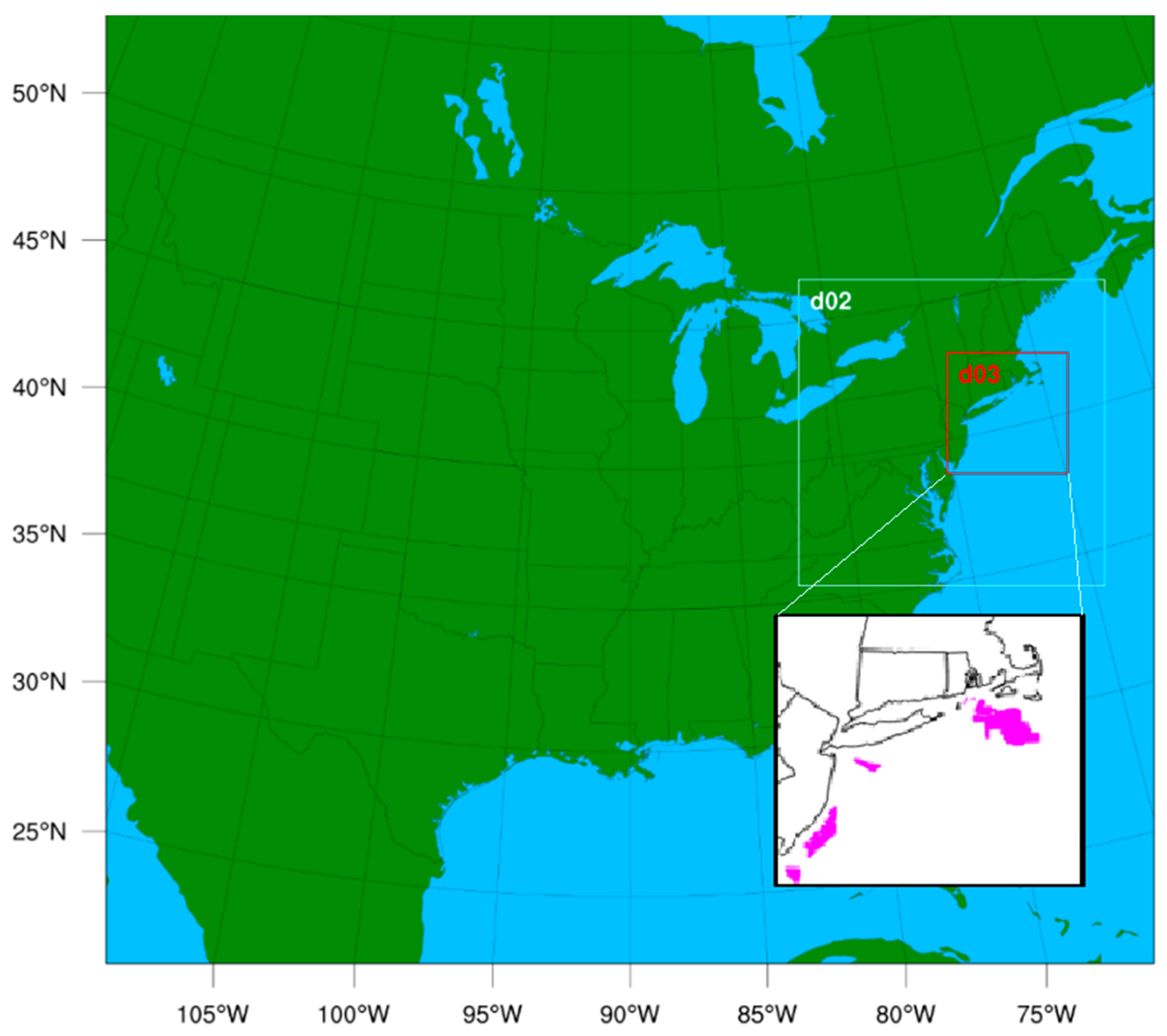
2.2. LLJ Analysis Domains

Wind speed components, potential temperature, and planetary boundary layer (PBL) height are analyzed from grid cells containing the centroid of each of thirteen active offshore wind energy lease areas (Figure 2). Results from the individual lease areas (LA) are clustered into four groups to examine the macroscale variability in LLJ characteristics. Group 1 encompasses seven lease areas and is centered south of Massachusetts. Group 2 is an individual lease area located in New York bight. Group 3 covers two lease areas off the New Jersey coast. Group 4, comprised of three lease areas, is the most southerly and is centered south of New Jersey and east of Delaware (Figure 2a).

Two transects are also constructed for LLJ analysis. Transect A comprises 9 points spaced at 40 km. It extends approximately 300 km west–east off the coast of New Jersey, and was constructed to analyze meso-scale variability in LLJ characteristics and specifically examine LLJ frequency as a function of fetch without the influence of other coastal landforms (such as Long Island or Cape Cod) (Figure 2b). Transect B was used to examine intra-farm variability and was sampled at nine points over a 30 km total length. Transect B is influenced by Long Island to the north and covers the entirety of the planned lease area off the coast of Long Island (NY Equinor). It is used to describe LLJ variability on an intra-wind farm scale (Figure 2c).

2.3. LLJ Detection and Characterization

2.3.1. LLJ Detection

LLJ frequency and characteristics are sensitive to the definition employed [50,51]. Use of only an absolute wind speed threshold for detection (i.e., maximum wind speed at the jet core exceeds that above and below the jet by X ms⁻¹) results in higher speed LLJs, whereas the use of only a relative (or variable) wind speed threshold (i.e., jet core wind speed exceeds wind speeds above and below by X%) results in lower speed LLJs [52]. A combination of relative and absolute threshold was employed here. An LLJ was identified at a given location and hour if the maximum wind speed from any vertical level (15–500 m a.s.l.) deviated from any speeds above and below by both (i) > 20% and (ii) > 2 ms⁻¹.

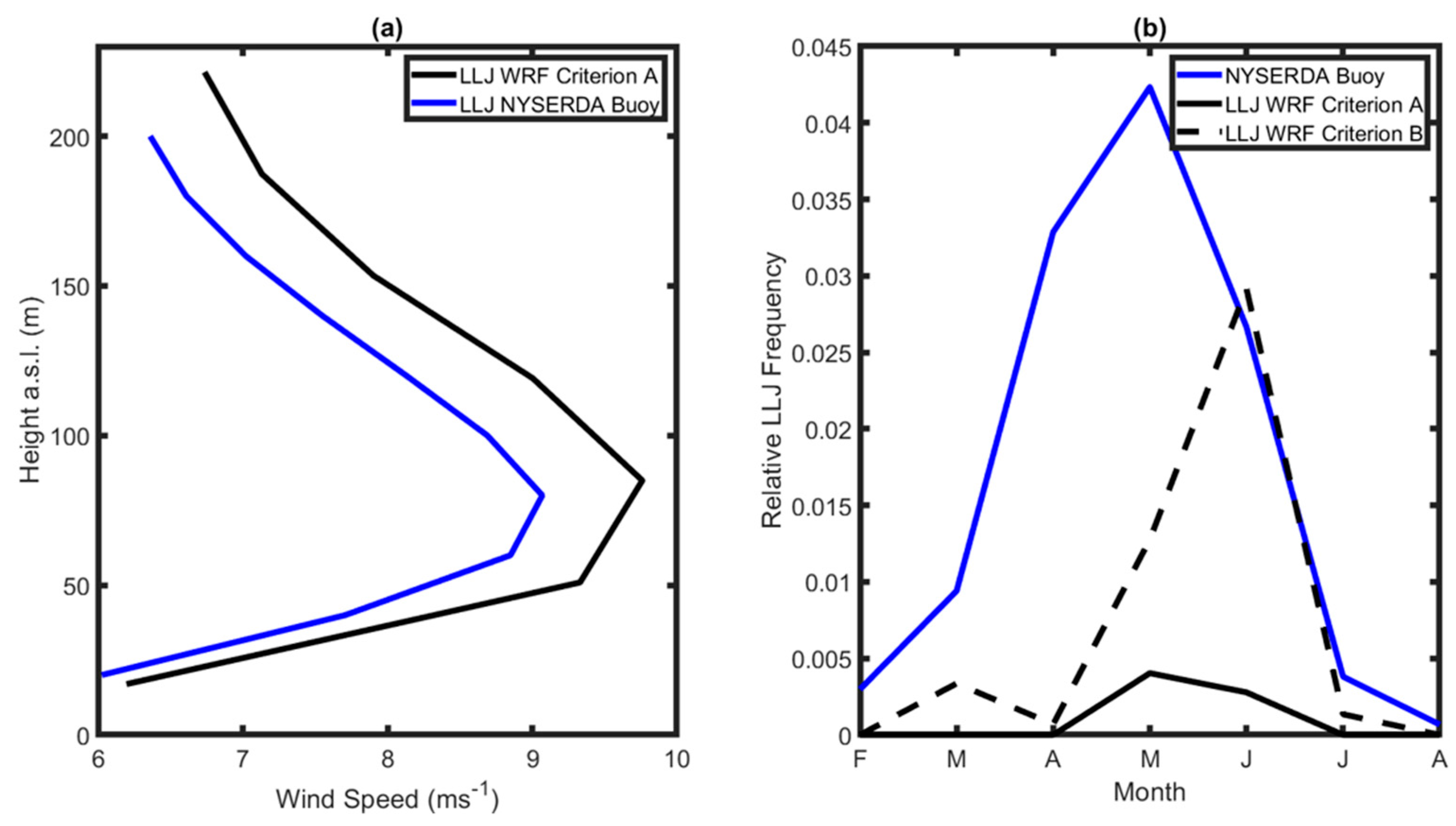
2.3.2. Preliminary WRF Simulation Validation

The LLJ climatology generated from the WRF output was evaluated using data from the buoy-mounted lidar closest to the centroid of the second lease area group (the NY Equinor lease area 39.97° N, 72.72° W). Because the lidar only measures wind speeds at heights of 20 to 200 m with a 20 m interval, in this comparison WRF output from the grid cell containing the buoy is sampled over the lowest 7 model levels (i.e., to 200 m a.s.l.) for comparability. Two LLJ extraction criteria are applied to compare seasonality between the WRF output and buoy data due to the low vertical window of the data (approximately 200 m a.s.l.): Criterion A, 1 ms⁻¹ and 10%; and Criterion B, 2 ms⁻¹ and 20%. Mean LLJ profiles and LLJ seasonality from seven months of the NYSERDA buoy data and WRF simulation are compared.

2.3.3. LLJ Characterization

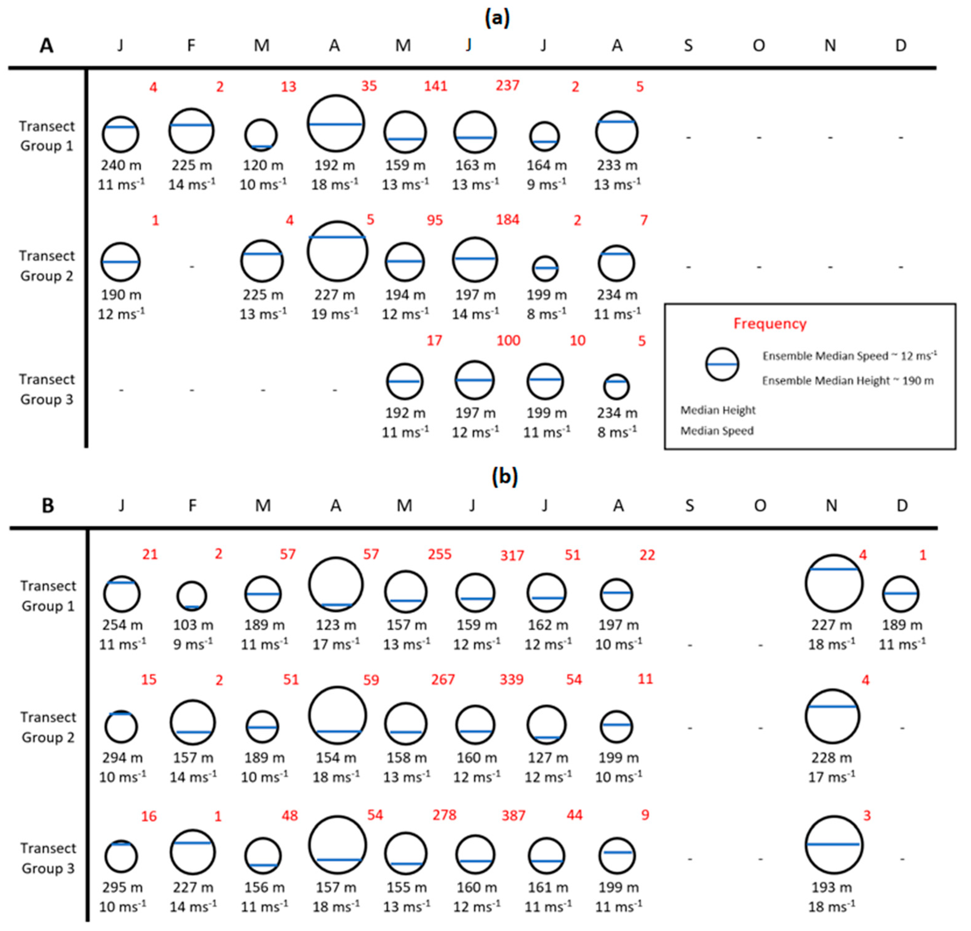
Following preliminary validation of the WRF simulation in resolving LLJs, LLJ characterization is outlined broadly as follows: spatiotemporal mean LLJ and non-LLJ wind speed profiles from each LA group are evaluated for the 2-year period to evaluate differences in the wind climate with changes in latitude. Following this, seasonal empirical probability distributions for LLJ occurrence across each LA group and transect group are presented. Next, monthly LLJ frequencies are further evaluated across the entire domain. For this analysis, wind speed profiles are sampled every three hours at every third grid point for computational efficiency, and monthly maps for relative monthly LLJ frequencies are produced across the domain. Because many of the variables considered herein are not Gaussian distributed, in much of the following the median is used as the primary measure of the central tendency of regional LLJ characteristics. However, to enable comparisons with past work, mean values are also cited for some LLJ properties. Where spatiotemporal median or mean values of wind speed, direction, horizontal potential temperature gradients, or PBL height (PBLH) are presented, the averaging is first performed for a given grid cell in time, and then averaged in space. Mean wind speed profiles for the LLJ and non-LLJ conditions are calculated from the mean wind speed components (u, v) at each vertical level during hours with and without LLJs. Where lease area centroids and transects are grouped (i.e., the four LA centroid groups and three groups per east–west transect as described in Figure 2), LLJ wind profiles are sampled for each group to create separate data subsets. From these subsets (4 subsets for each LA centroid group and 3 subsets across each transect), LLJ statistics and characteristics are calculated.

After the investigation of LLJ ensemble characteristics, four key aspects of LLJs and their occurrence are presented herein via joint distributions and conditional probabilities. Each joint distribution extends the initial LLJ characterization and investigates the probability of conditions in which they occur (probability of jet core speed and height, spatial extent, diurnal variability and seasonality of occurrence, variations in wind direction during LLJ occurrence):

(i)

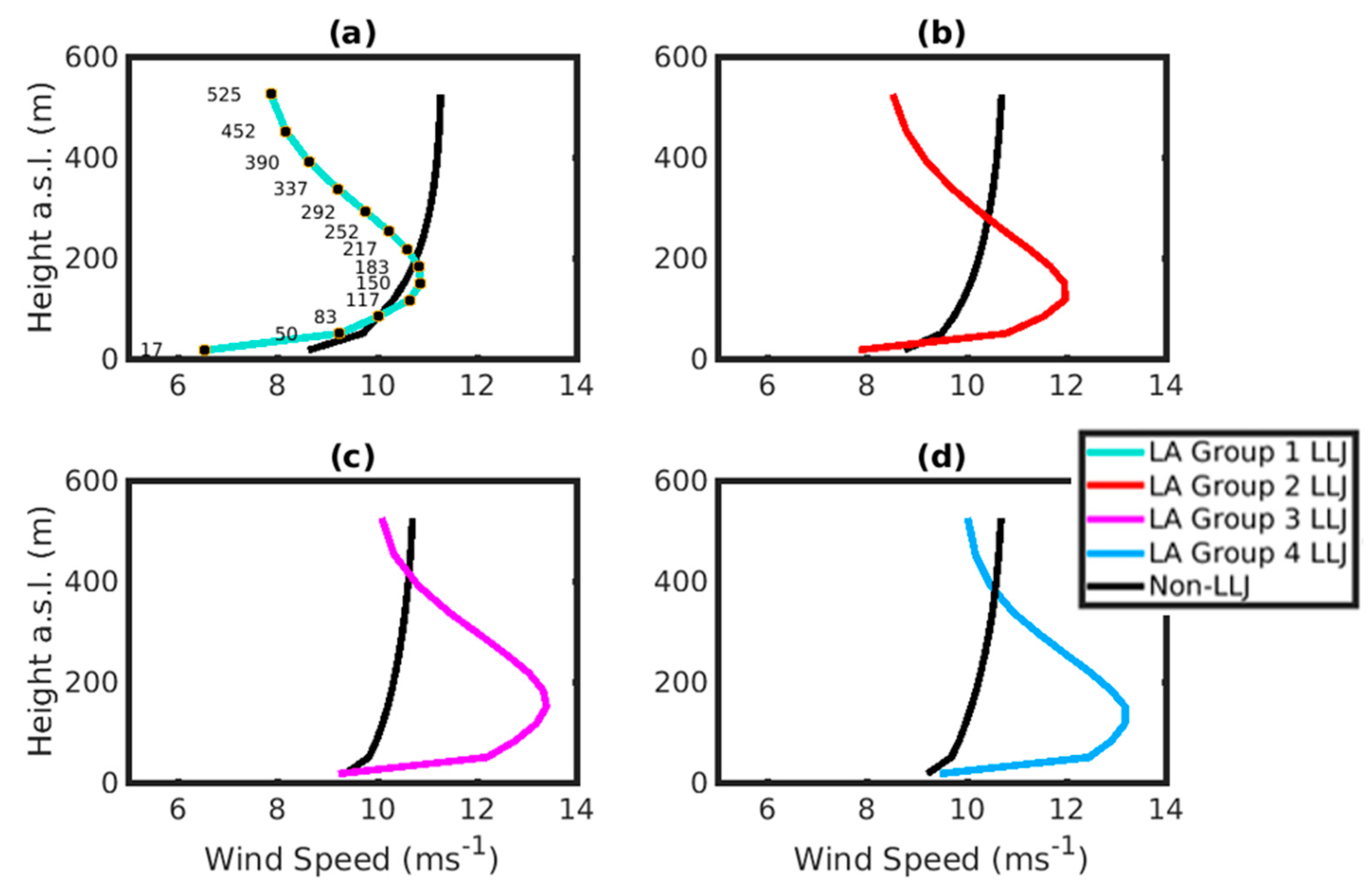
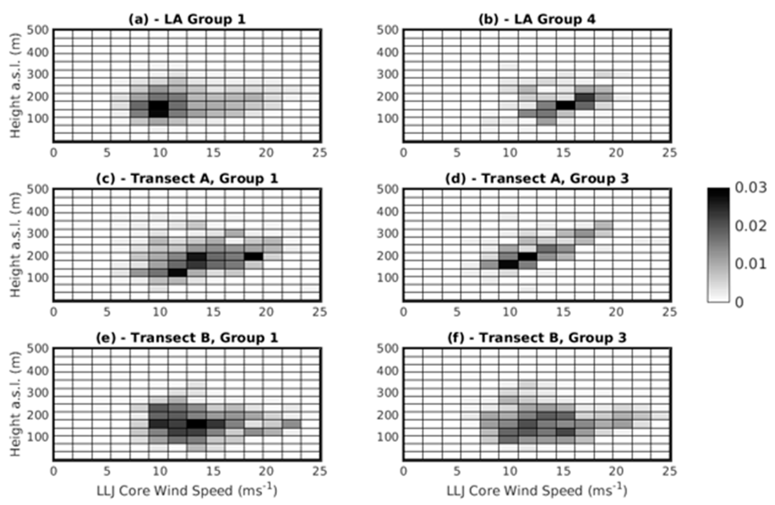
Joint probability distributions of LLJ core heights and speeds are analyzed across the selected LA groups and transect groups to examine how LLJ characteristics change with latitude and distance from the coast (macro- meso- and intra-farm scales). This analysis is performed for transect groups closest to the coast and farthest from the coast for both transects (Groups 1 and 3), plus LA groups 1 (south of MA) and 4 (highest and lowest latitude, respectively).

(ii)

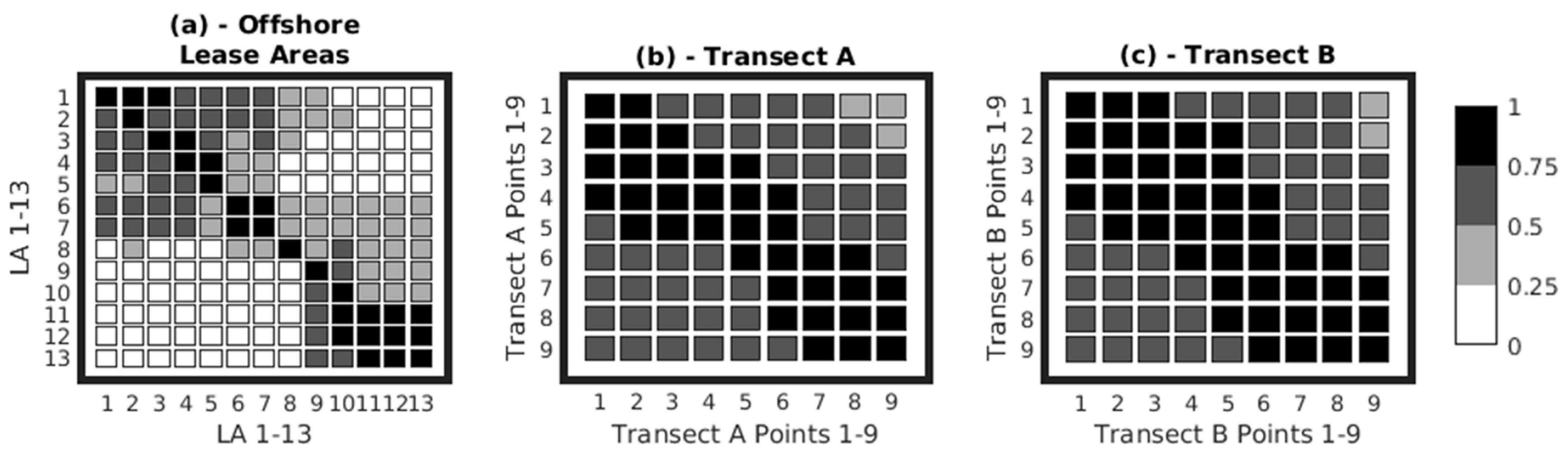
Spatial extent (i.e., co-occurrence in space). In this analysis, conditional probabilities of LLJ occurrence are calculated for each LA centroid and/or each pair of points along both transects. For example, for transect A, the conditional probability is calculated that, if a LLJ is detected at point 1 (closest to the coast) in one hour, a LLJ will also occur at point 9 (farthest from the coast) in that same hour.

(iii)

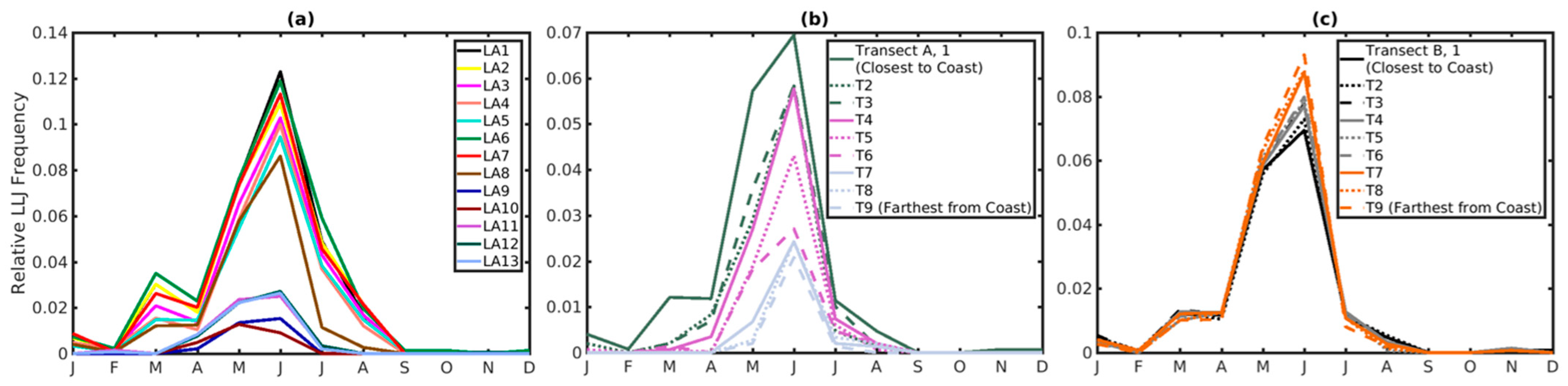
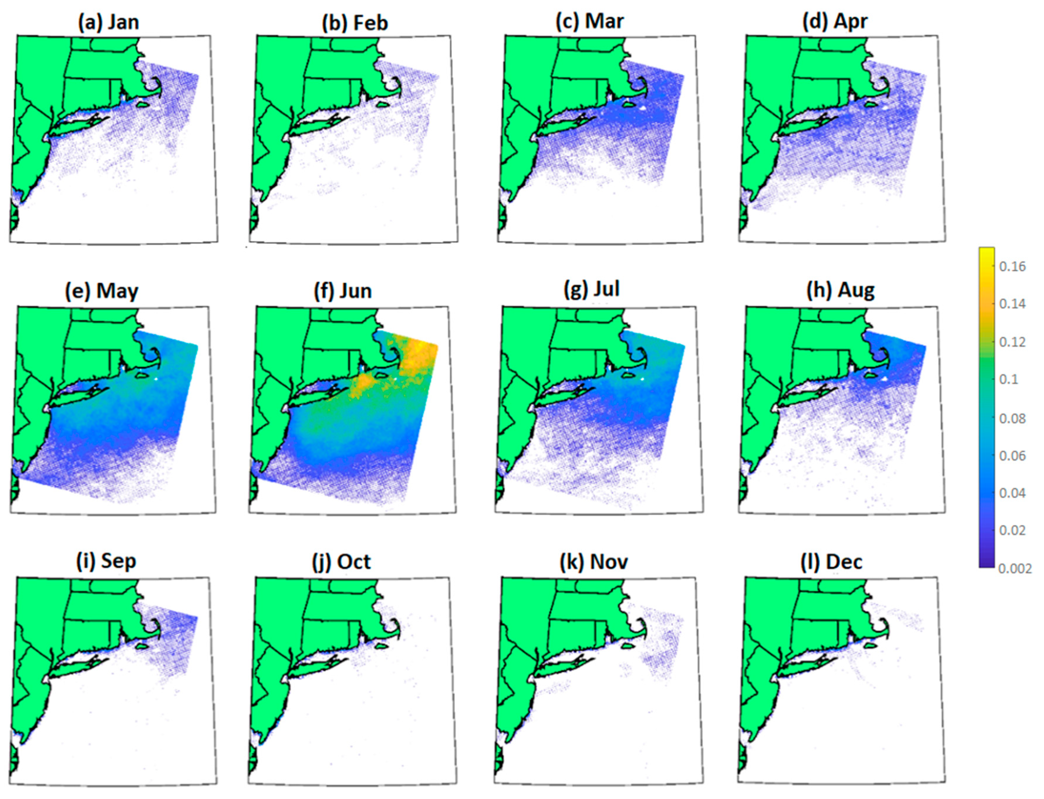
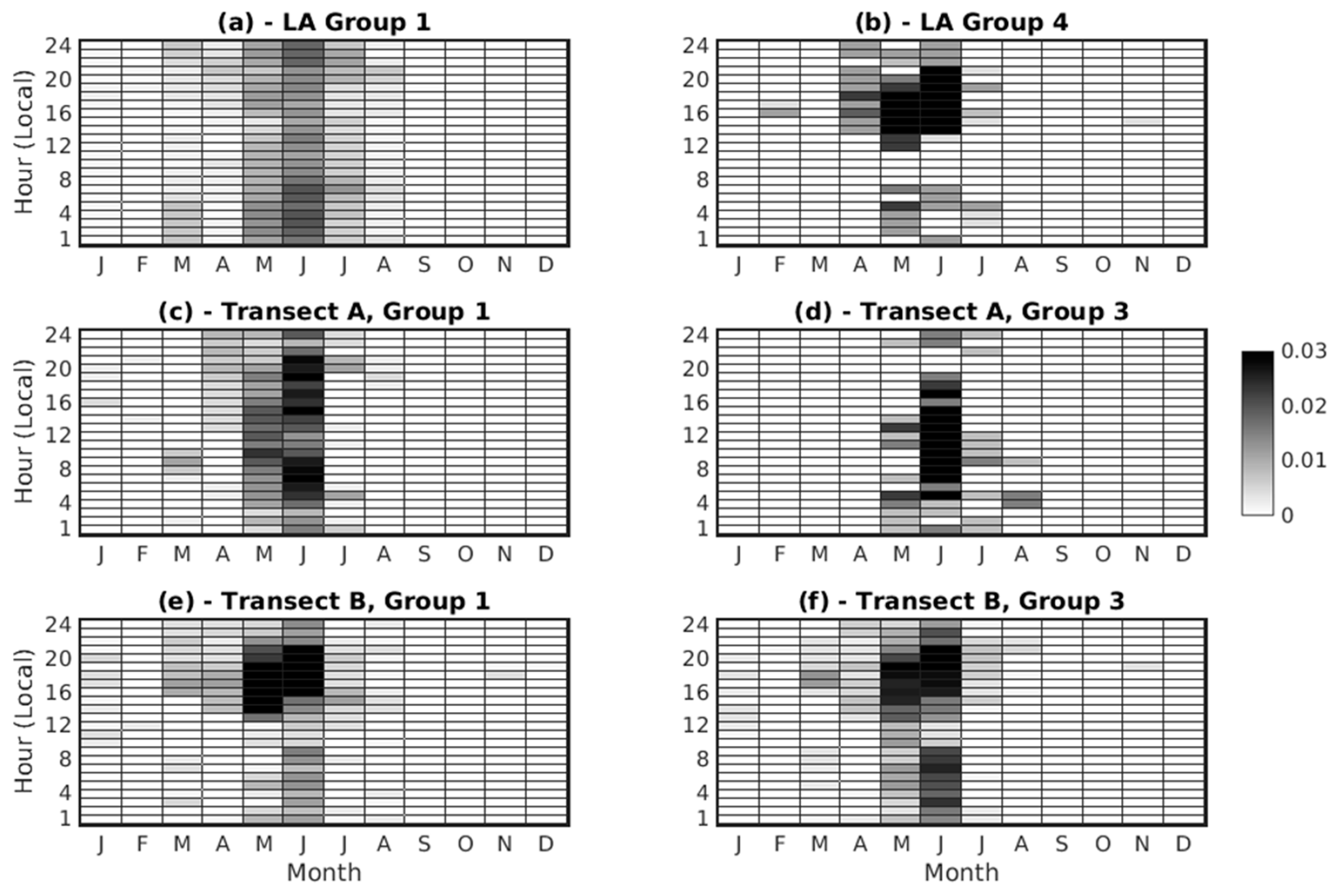
LLJ probability of occurrence as a function of hour of the day and calendar month.

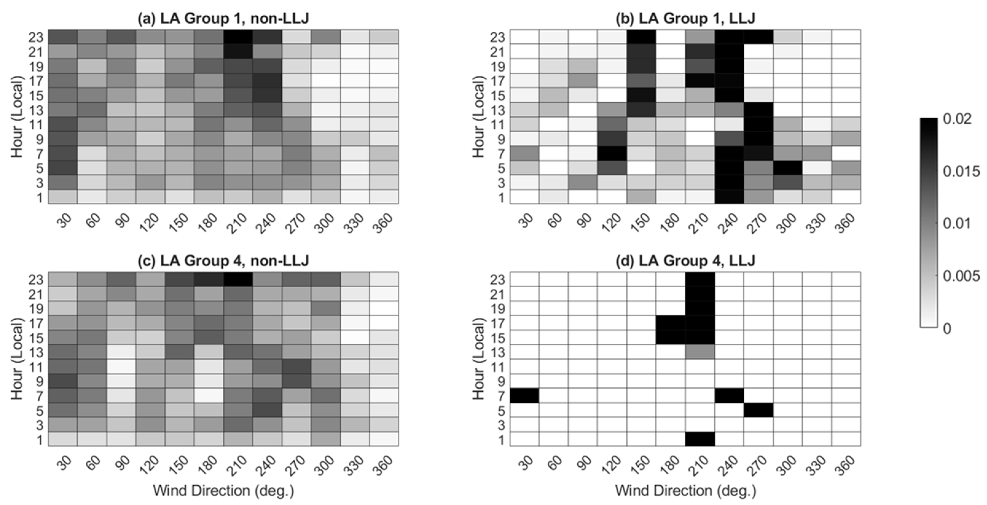
(iv)

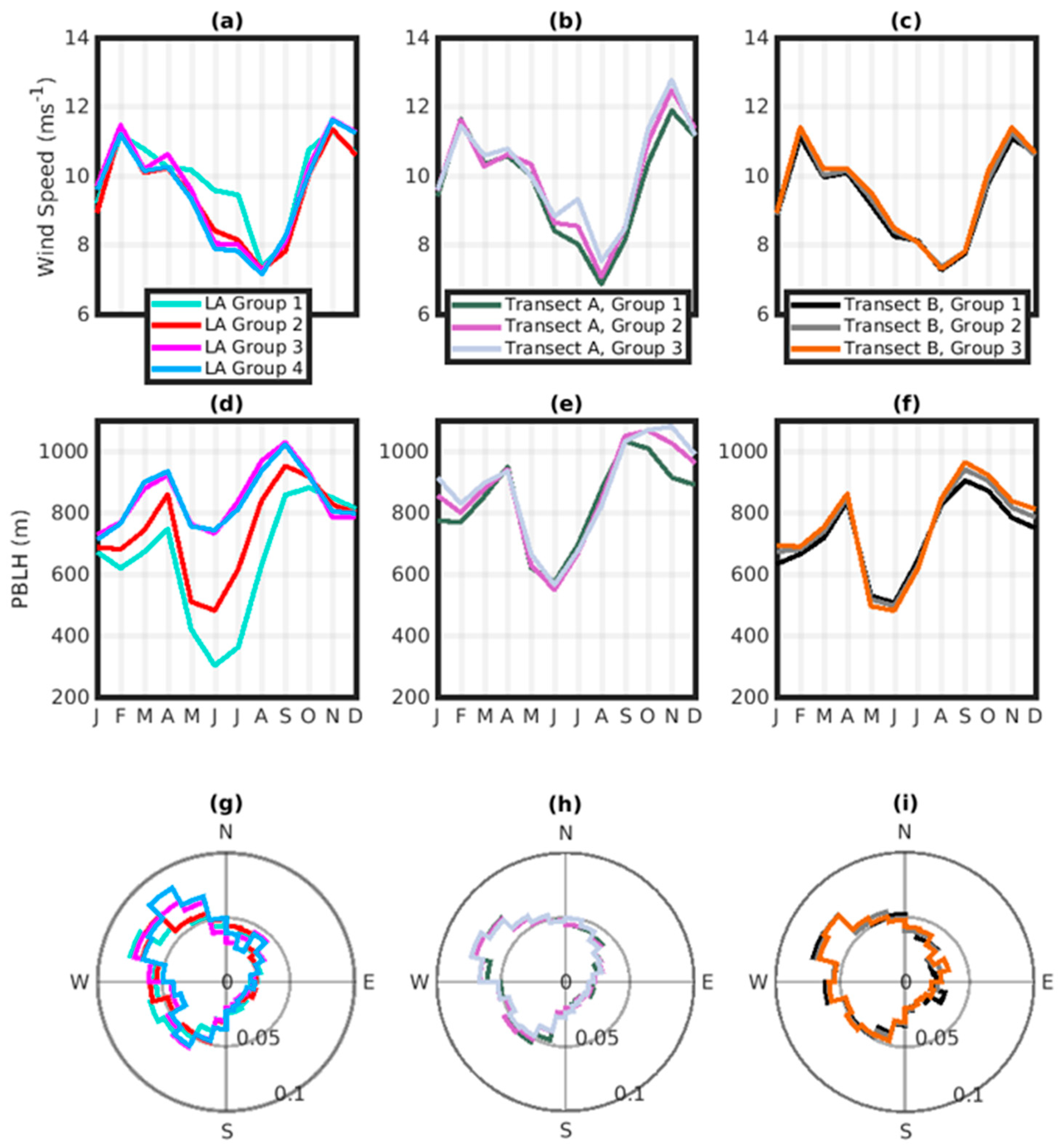
Joint probability distributions are constructed for LLJ occurrence considering both hour of the day and wind direction at ~100 m for the month of highest LLJ frequency (June). This analysis focused on two LA groups. Probabilities of LLJs in the first group (LA group 1 in the north) are almost exclusively confined to the evening hours to early morning hours (approximately 8 pm–8 am, local time) in June. Conversely, for this month, probabilities of LLJs in the second (LA group 4 in the south) do not follow a pronounced diurnal cycle.

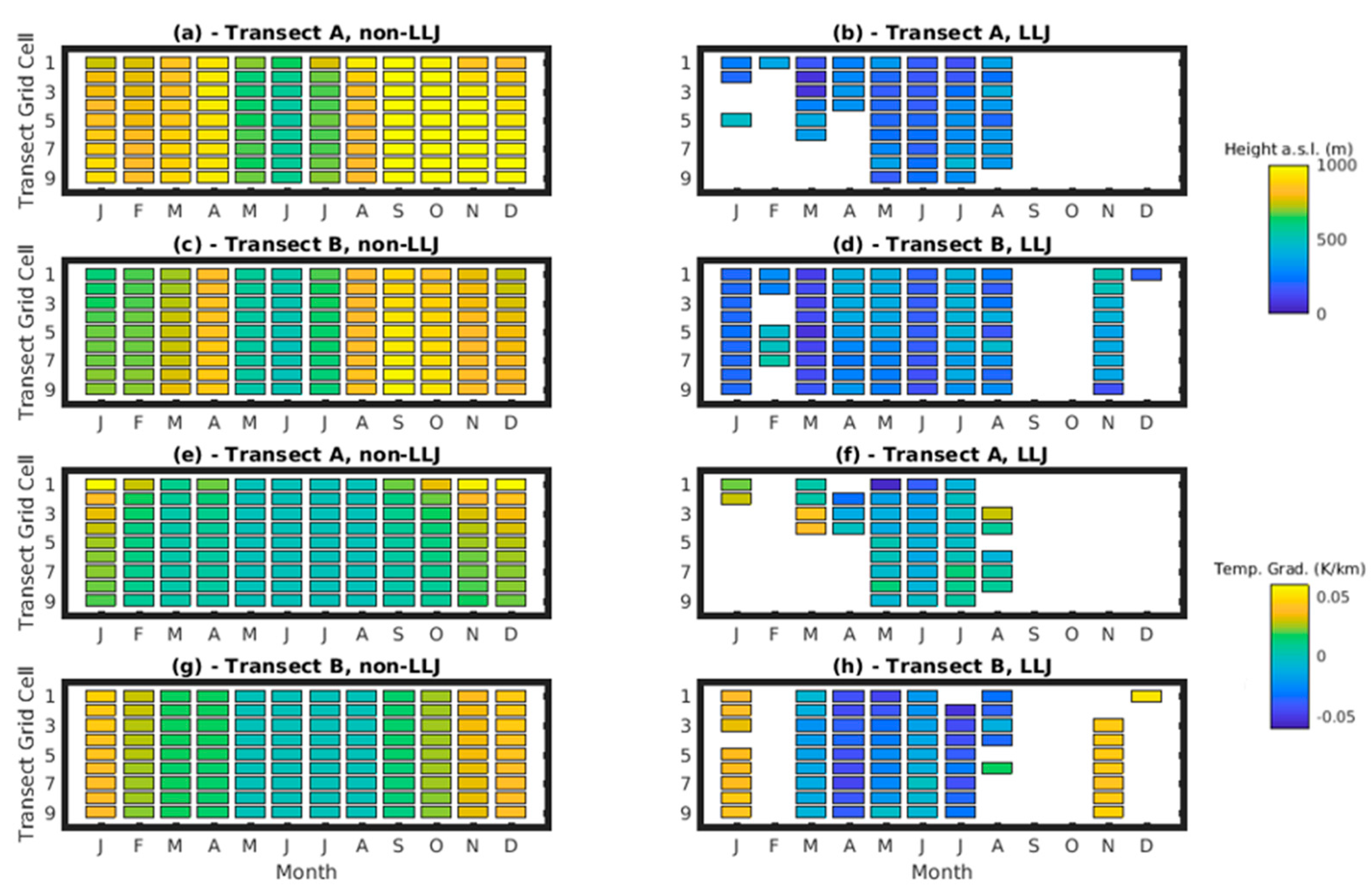
2.3.4. Analysis of Meteorological Conditions associated with LLJs

The probability of occurrence and LLJ characteristics are analyzed with respect to two key meteorological variables; horizontal land–sea gradients of potential temperature (θ) at the sixth WRF sigma level (~180 m a.s.l., corresponding to the value of the median jet core height) and PBLH along the two transects (Figure 2b,c). Horizontal gradients of potential temperature are calculated every three hours at each point along each transect (X_i) relative to output from the reference land grid cell denoted in Figure 2 (X_ref = 0):

$${\frac{\Delta \theta }{\Delta X}}_i=\frac{{\theta }_i-{\theta }_{ref}}{X_i-X_{ref}}$$

(1)

PBLH is analyzed hourly and is as defined within the MYNN scheme as the lowest height at which modeled turbulent kinetic energy (TKE) < 1.0 × 10⁻⁶ m²s⁻² [51].

Mann–Whitney U tests [53] are used to evaluate the null hypothesis that PBLH or potential temperature gradients in the non-LLJ and LLJ samples are from the same population. Rejection of the null hypothesis at the 95% confidence level indicates that, for a given month, horizontal temperature gradients or PBLH associated with LLJ and non-LLJ conditions are drawn from different populations, and thus that PBLH and/or horizontal gradients of temperature are causally linked to LLJ occurrence.

After significance testing of climatological conditions associated with LLJ occurrence, LLJs are characterized monthly for each subset in terms of median LLJ core height, frequency (for hourly realizations of wind speed profiles), and wind speed. LLJ characteristics are then analyzed relative to the significance of climatological conditions associated with their development, i.e., median LLJ characteristics for months in which the LLJ gradients are deemed significant according to the Mann–Whitney U-Tests are compared to median characteristics during months without significant temperature gradients.

3. Results

3.1. Wind Climate

Consistent with previous independent WRF simulations and satellite-based remote sensing [13], wind speeds output for all lease area (LA) centroids and transect groups exhibit lower values in the warmer months (Figure 3a–c). The median wind speed at ~100 m a.s.l. is <8 ms⁻¹ in August, whereas values during the winter months are approximately 11–12 ms⁻¹. Transect A (extending west–east off the coast of New Jersey, NJ, see Figure 2) exhibits highest seasonality. Median wind speeds in August and November differ by 80% of the August value. The seasonal variability of wind speeds at the individual LA or along transects exceeds the spatial variability in the annual wind speeds. For the LA south of Massachusetts (LA group 1), the mean annual wind speed at 100 m is approximately 9.89 ms⁻¹, whereas it is 9.55 ms⁻¹ for the southernmost lease areas (LA group 4) off the coast of Delaware. There are also only modest differences in average wind speed across the transects (i.e., with distance to the coast). For transect A (340 km long) and B (40 km long), annual mean wind speeds at ~100 m a.s.l. increase by 0.0014 and 0.0057 ms⁻¹ per km from the coast, respectively. This is consistent with the largest wind speed gradients occurring within 40 km of the coastline as the flow adjusts to the lower surface roughness and the changing surface energy fluxes. All groups exhibit predominantly northwesterly and southwesterly flows with few observations from the southeast.

PBLHs also exhibit a profound seasonal cycle and spatial variability (Figure 3). For all LA and transect groups considered, highest median PBLHs occur during transition months (spring and fall), in agreement with lidar observations [54]. PBLHs are lower during summer due to advection of warmer air over the cooler sea surface. Lease area groups at lower latitudes that also have shorter over-water fetches in the dominant wind direction exhibit higher median PBLHs than those of LA groups 1 and 2 (Figure 3h–i). There is also marked variability in PBLH across the transects in fall (September–November, inclusive).

3.2. Preliminary WRF Simulation Validation

Depicted in Figure 4, mean LLJ profiles extracted from the buoy-mounted lidar in the lowest 200 m a.s.l. exhibit similar mean jet core heights but slightly lower mean jet core speeds than LLJs extracted with the same definition (Criterion A) from the first 220 m a.s.l. of WRF output (corresponding to the lowest 7 sigma levels). The mean values for jet core speed and height from the buoy are 9.1 ms⁻¹ and 80 m a.s.l., whereas values from WRF are 9.8 ms⁻¹ and 84 m a.s.l. (Figure 4a). Both datasets indicate relatively low monthly LLJ frequencies (Figure 4b). When LLJs are extracted with Criterion A, LLJ frequency is comparatively low in magnitude but exhibits a peak in the warm months (Figure 4b). When LLJs are extracted from the lowest 7 sigma levels of WRF output under Criterion B, the absolute frequency of LLJ occurrence increases in magnitude and peaks in the warm season. Thus, the absolute magnitude of monthly frequency is sensitive to the LLJ definition employed (particularly due to the limit of the low vertical window) but the peak of LLJs in the warm season is well-resolved. Some discrepancies may be further explained by inter-annual variability of LLJ frequency and characteristics, because the lidar data only cover 7 months whereas the WRF output covers 2 years.

3.3. LLJ Identification and Characterization

Mean wind speed profiles conditionally sampled by the presence or absence of LLJs exhibit pronounced spatial variability across the LA groups (Figure 5). The mean profiles when LLJs are absent have an approximately logarithmic form. Output for LA group 1 non-LLJ (south of Massachusetts) exhibits more vertical shear and higher wind speeds at ≈100 m a.s.l. For LA group 1, the mean LLJ core wind speed is 10.9 ms⁻¹, whereas LA groups 2, 3, and 4 exhibit higher mean jet core speeds of 12.0, 13.4, and 13.2 ms⁻¹, respectively. Importantly in a wind energy context, the spatiotemporal mean heights of the LLJ cores are below 200 m a.s.l. for all LA groups, indicating that LLJs tend to occur within or near the nominal wind turbine rotor plane. LA groups 1, 2, 3, and 4 exhibit spatiotemporal mean jet core heights of 170, 157, 172, and 160 m a.s.l., respectively. Weibull distribution fits to hourly wind speeds at ~100 m a.s.l. during LLJs indicate LLJs exhibit very similar shape (k) and scale (c) parameters. For example, in output from LA group 1, k = 1.997 and c = 11.93 ms⁻¹ when LLJs are absent, and k = 2.013 and c = 11.94 ms⁻¹ when LLJs are identified as present. The implication is LLJs may have comparatively little impact on the wind resource close to hub-height but may have a greater impact on rotor equivalent wind speeds and/or shear across the rotor plane.

LLJs are most frequent over all LA and transects during the summer months (Figure 6). The highest probability of occurrence is found for LA group 1 (south of Massachusetts), with LLJs occurring in up to 12% of hours during June. LLJs are least frequent at LA off the Maryland coast (Figure 6). Along transect A, highest jet frequencies (up to 7% of all time periods) are observed approximately 30 km off of the coast (T1) with a decrease in frequency with increasing distance from the coast across all months considered. However, along the shorter near-coastal transect (B), as distance from the land increases, LLJ frequency increases for warmer months and there is less evident spatial variability in the winter. At approximately 60 km from the coast along transect B, frequency increases to 9% of all hours in June (T9). This re-emphasizes the multiple scales of influence on LLJ frequency and characteristics (i.e., sea breeze circulations vs. the role of capes and peninsulas). The increase in LLJ frequency in the warm months may be attributed partially to differences in land–sea horizontal temperature gradients observed in these months (and described in Section 3.5).

To provide a geospatial context for the LLJ frequencies in the LA, the same detection algorithm was applied to 3-hourly output sampled at every third grid cell in the domain (Figure 7). The results emphasize the summer peak in LLJ frequency and indicate LLJs are identified in output from nearly every grid cell of the domain (Figure 7). During the warm months, LLJs are observed throughout the majority of the domain, whereas from October to December LLJs are infrequent everywhere. LLJ frequency is particularly high in the Cape Cod, Nantucket Sound, and Cape Ann regions (i.e., near the state of Massachusetts). During June, LLJs are identified in these regions in up 18% of hours. LLJ frequency generally declines with decreasing latitude during both warm and cool months, although areas of Long Island Sound (near LA group 2) exhibit relatively high LLJ frequency in both warm and cool months. Thus, spatial patterns in LLJ frequency are dependent on both month and location within the domain, further validating the results in Figure 6.

3.4. Extended Analysis of LLJ Characterization

Joint probability distributions of LLJ core height and magnitude indicate most jets identified using the criteria described above occur within the likely wind turbine rotor plane (heights 50–250 m) and at wind turbine operating conditions (i.e., wind speeds above cut-in and below cut-out) (Figure 8). LA group 1 has the highest LLJ frequency (Figure 6) and a clear maximum rate of occurrence with LLJ core wind speeds of approximately 10 ms⁻¹ and core heights of 100–170 m a.s.l. (Figure 8). Conversely, WRF output for LA group 4 (the most southerly), indicates a low frequency of LLJs (Figure 6) and a clearer association between LLJ intensity (wind speed) and core height (Figure 8). Higher core heights are generally associated with higher LLJ core wind speeds. There is a clear decrease in LLJ frequency with distance offshore along transect A (Figure 6), and LLJs further from the coast also appear to be associated with lower core wind speeds (Figure 8). Across the shorter transect B, LLJs occur at similar heights and with similar jet core wind speeds.

LLJs exhibit spatial coherence over tens of kilometers but the probability of co-occurrence greatly declines with greater separation (Figure 9). The mean separation of the LA centroids in the cluster south of Massachusetts (LA 1–7) is 28 km. When a LLJ is detected in one of these LA centroids, it is highly likely (0.50 < p < 0.75) that a LLJ will be detected concurrently at the centroid of other nearby lease areas (LA 1–7) (Figure 9a). For lease area centroids 11–13 (Figure 2), which are in closer proximity to each other, it is highly likely (p > 0.75) that if a LLJ is detected at one centroid, there is a LLJ is detected at the other centroids. Thus, based on this analysis of WRF output, whereas LLJs are detected in relatively few hours on average, LLJs are highly likely to simultaneously impact multiple nearby lease areas.

Intra-transect conditional probabilities of concurrent LLJs are also high (p > 0.5). In over three-quarters of time periods when a LLJ is detected at one point along transect A, a LLJ is simultaneously indicated in grid cells displaced up to 120 km east and west of it (Figure 9). There is asymmetry of conditional probabilities in both transects. It is less likely if a LLJ occurs at the transect point closest to the coast that it will also occur further offshore than vice-versa. These asymmetries are further evidence that LLJ generation in the region occurs across multiple scales from intra-farm to meso-scale.

Joint probability distributions for LLJ occurrence by month and hour illustrate the dominance of the seasonal cycle over the diurnal cycle in terms of frequency with which LLJs are manifest (Figure 10); that is, there is a more consistent seasonal cycle (with a peak in the warm months) for LLJs across the domain, whereas there is evidence of intermittent diurnal signals in LLJ appearance depending on location and season. For LA group 1, transect A group 1 (approximately 40 km from the coast) and transect B group 3 (approximately 50 km from the coast), LLJs are observed during all hours of the day in May and June. LA group 1 exhibits a higher probability of LLJ occurrence overnight and in the evening. For the more southerly lease areas (LA group 4), the variability in the frequency of occurrence with hour of the day is even more pronounced. At LA group 4, there is a clear evening peak in LLJ occurrence. The presence or absence of a diurnal cycle in LLJ occurrence may be related to diurnal variability in flow direction and the proximity to land as described further below.

LA group 1 has west–east and south–north oriented coastlines to the north and west, respectively. WRF output for this location during June indicates the highest frequency of LLJs under west-southwesterly (240°) and southeasterly (120°) flows at ~100 m a.s.l. (Figure 11). Thus, LLJs are most frequently observed when the flow is nearly parallel to the coastlines. Output for LA group 4 (off a south–north oriented coastline) exhibits LLJs that are preferentially associated with south-southwesterly flow (Figure 11). This is again almost parallel to the closest coastline (to the west, see Figure 1).

LLJ characteristics across the two transects (A and B) are summarized in Figure 12. Recall, transect A extends over 300 km from the closest coastline, whereas transect B is used to describe intra-wind farm variability and thus extends only 40 km. Across the intra-farm transect B, median LLJ core height in peak months (April, May, June, July) is lower than in other months, indicating that, during the months of highest frequency, LLJs are likeliest to interact with the rotor plane. LLJs occur with higher jet core heights in the cooler months. Further, for transect A, jet height increases with distance from the coast, with LLJs closest to the coast exhibiting lowest heights for nearly all months. Increases in jet height with increasing distance from the coast are similarly observed for transect B, particularly for cooler months and into the early warm season (Jan–April).

3.5. Meteorological Context for LLJs

Boundary layer heights during periods with LLJs are consistently lower, on average, than hours in which LLJs do not occur (Figure 13). Median PBLHs during LLJ occurrence across all months for transects A and B are 277 and 299 m a.s.l., respectively, whereas median PBLHs during non-LLJ conditions for transects A and B are 864 m and 760 m a.s.l., respectively. This may reflect the importance of frictional decoupling at the top of the PBL and occurrence of super-geostrophic flow in generating LLJs [55]. Although PBLHs vary markedly with season (Figure 3), this association between lower PBLH and higher LLJ frequencies is maintained.

Thermal gradients associated with LLJ occurrence are characterized using the gradient in potential temperature (θ) close to the median LLJ core height of 180 m a.s.l. from the coast and at each point along transects A and B (i.e., increasing x, as described in Equation (1), indicates further offshore). The median horizontal gradients of potential temperature (Δθ/ΔX) across transects A and B during non-LLJ hours are positive (higher θ further offshore) during the winter months, and close to zero during the summer (Figure 13). LLJ occurrence during the summer is generally associated with negative horizontal potential temperature gradients (colder temperatures further offshore). This is consistent with warmer air temperatures over land surfaces during the day and a contribution from the thermal wind to LLJ generation. As noted by [49], the occurrence of LLJs mainly in the summer “supports a baroclinic contribution and possibly an interplay with the evolution of sea breezes”.

Mann–Whitney U-tests applied to land–sea horizontal potential temperature gradients and PBLH during each calendar month indicate median values of Δθ/ΔX and PBLH are generally significantly different for non-LLJ and LLJ periods (Figure 14). Median Δθ/ΔX during LLJ and non-LLJ occurrence is not statistically significant in data from across the two transects in all months, but median PBLHs are frequently significantly lower when LLJs are detected.

For months in which LLJ occurrence is linked to variations in horizontal land–sea potential temperature gradients, LLJs exhibit marked spatial variability across both transects, in terms of frequency of occurrence, maximum wind speed and jet core height (Figure 12, Figure 13 and Figure 14). Along transect A, LLJs exhibit higher median jet core wind speeds during months when the potential temperature gradients differ most from the “background” (i.e., the median value from the sample of non-LLJ cases). In months when the median horizontal gradient of potential temperature differed from that in non-LLJ periods, the median LLJ core wind speed on transect A is 12.6 ms⁻¹, whereas for months where the median Δθ/ΔX in the LLJ and non-LLJ samples do not differ, it is 11.0 ms⁻¹. The same is observed for transect B, which exhibits jet core speeds of 12.4 and 10.6 ms⁻¹, respectively. This may imply that, although the dominant mechanism of formation is linked to frictional decoupling, the LLJ intensity is being enhanced by the thermal wind.

4. Summary and Conclusions

Data availability on flow conditions over and in the coastal zone along the U.S. east coast is sparse, although the United States plans to install nearly 30 GW of offshore wind energy capacity in this region by 2030. To aid in filling this data gap, 2 years of high-resolution WRF simulations were performed and analyzed. The analyses focus on characterizing the wind climate and coastal LLJ characteristics and spatial and temporal frequencies in the current generation of offshore lease areas and along two transects extending from the coastline (Figure 2). The 13 active offshore lease areas examined here are clustered into four groups—group 1: LA 1–7 south of Massachusetts; group 2: LA 8 off the east coast of New York state; group 3: LA 9–10 off the coast of New Jersey; and group 4: LA 11–13 (further south) (see Figure 2). Transect A is a nine point east–west transect located off the coast of New Jersey extending approximately 300 km from the coast. Transect B also comprises nine equidistant points but has a spatial extent of approximately 30 km near Long Island in the New York bight region. This transect crosses the extent of the New York Equinor lease area and was designed to examine LLJ variability at the intra-farm scale.

Wind speeds close to 100 m a.s.l. are lower in the warmer months, with median monthly values around 8 ms⁻¹ (warmer months) to 11 ms⁻¹ (winter months) throughout the study region. Wind directions in each lease area group are found to be dominated by northwesterly and southwesterly flows.

LLJs are identified from the hourly WRF output as vertical profiles where a wind speed maximum is evident in the lowest 530 m of the column and wind speeds are 20% and 2 ms⁻¹ lower both above and below that height. This analysis fully encompasses the height of the rotor plane of all currently available wind turbines. A similar analysis was also applied to output from WRF for the lowest 200 m a.s.l. and a vertically scanning lidar on a buoy in the New York Bight region. These analyses indicate relatively good agreement between the LLJ jet core height and wind speed and seasonality from the lidar and WRF, with peak LLJ frequency in the warm season (May–September). LLJ occurrence is highest in June for all groups of LA and indeed over the entire simulation domain. LLJs are detected most frequently in the northern-most lease areas located south of Massachusetts (LA 1–7). This region shows LLJs in up to 12% of hours in June, with winter exhibiting comparatively low LLJ frequency (Figure 5). LLJs also exhibit a high probability to occur at rated wind speeds for turbines planned in the region, with all domains exhibiting relatively high probability of LLJs occurring with jet cores of 10 ms⁻¹ or higher. Generally, LLJ frequency decreases with decreasing latitude, but increases or decreases with increasing fetch, depending on the location within the domain. For all locations considered, LLJ cores are frequently found at heights that intersect wind turbine rotor planes; the median LLJ height is ~150 m a.s.l. in all LA groups. LLJ characteristics (speed, height) exhibit less variation on the intra-farm scale (across transect B) when compared to meso- (transect A) or inter-farm (across lease area groups) scales.

Co-occurrence of LLJs in space (i.e., in grid cells of varying horizontal separation) was used to characterize the spatial scales of LLJs. LLJs typically do not simultaneously impact the southern-most and northern-most LA groups. Although LLJs are most frequent in the northern LA group, there is clear evidence LLJs are less likely to occur simultaneously in this region than in the southern-most LA group, which exhibits high probability of jet co-occurrence.

Although there is clear seasonality in LLJ frequency, variability with hour of the day is considerably more modest. LLJs are preferentially found to be aligned with the nearest coastline. For all transect and LA groups, LLJ occurrence is associated with lower boundary layer heights and negative horizontal land-sea potential temperature gradients (cooler conditions offshore) during the summer months. Future work will include investigation of the impact of LLJs on rotor equivalent wind speed and shear across the rotor plane, in addition to further investigation of causal mechanisms of LLJs for the region.

References

1. Energy Secretary Granholm Announces Ambitious New 30GW Offshore Wind Deployment Target by 2030. Available online: https://www.energy.gov/articles/energy-secretary-granholm-announces-ambitious-new-30gw-offshore-wind-deployment-target (accessed on 10 October 2021).
2. Barthelmie, R.J.; Dantuono, K.E.; Renner, E.J.; Letson, F.L.; Pryor, S.C. Extreme Wind and Waves in US East Coast Offshore Wind Energy Lease Areas. Energies 2021, 14, 1053. [Google Scholar] [CrossRef]
3. U.S. Offshore Wind Power Economic Impact Assessment. American Clean Power Association. Available online: https://supportoffshorewind.org/wp-content/uploads/sites/6/2020/03/AWEA_Offshore-Wind-Economic-ImpactsV3.pdf (accessed on 10 October 2021).
4. Pryor, S.C.; Barthelmie, R.J.; Shepherd, T.J. Wind Power Production from Very Large Offshore Wind Farms. Joule 2021, 5, 2663–2686. [Google Scholar] [CrossRef]
5. Record of Decision, Vineyard Wind 1 Offshore Wind Energy Project Construction and Operations Plan. Bureau of Ocean Energy Management. Available online: https://www.boem.gov/sites/default/files/documents/renewable-energy/state-activities/Final-Record-of-Decision-Vineyard-Wind-1.pdf (accessed on 10 October 2021).
6. Pryor, S.C.; Barthelmie, R.J. Comparison of Potential Power Production at On- and Offshore Sites. Wind Energy 2001, 4, 173–181. [Google Scholar] [CrossRef]
7. Pryor, S.C.; Barthelmie, R.J. Statistical Analysis of Flow Characteristics in the Coastal Zone. J. Wind Eng. Ind. Aerodyn. 2002, 90, 201–221. [Google Scholar] [CrossRef]
8. Vickers, D.; Mahrt, L. Observations of Non-Dimensional Wind Shear in the Coastal Zone. Q. J. R. Meteorol. Soc. 1999, 125, 2685–2702. [Google Scholar] [CrossRef]
9. Barthelmie, R.J.; Hansen, O.F.; Enevoldsen, K.; Højstrup, J.; Frandsen, S.; Pryor, S.C.; Larsen, S.; Motta, M.; Sanderhoff, P. Ten Years of Meteorological Measurements for Offshore Wind Farms. J. Sol. Energy Eng. 2005, 127, 170–176. [Google Scholar] [CrossRef]
10. NYSERDA Announces Contracts for Collecting Environmental and Metocean Data in Support of Offshore Wind Energy Development—NYSERDA. Available online: https://www.nyserda.ny.gov/About/Newsroom/2019-Announcements/2019-01-31-NYSERDA-Announces-Contracts-for-Collecting-Environmental-and-Metocean-Data-in-Support-of-Offshore-Wind-Energy-Development (accessed on 10 October 2021).
11. Papadopoulos, P.; Coit, D.; Azizezzat, A. Seizing Opportunity: Maintenance Optimization in Offshore Wind Farms Considering Accessibility, Production, and Crew Dispatch. IEEE Trans. Sustain. Energy 2021, 13, 111–121. [Google Scholar] [CrossRef]
12. Debnath, M.; Doubrawa, P.; Optis, M.; Hawbecker, P.; Bodini, N. Extreme Wind Shear Events in US Offshore Wind Energy Areas and the Role of Induced Stratification. Wind Energy Sci. 2021, 6, 1043–1059. [Google Scholar] [CrossRef]
13. Ahsbahs, T.; Maclaurin, G.; Draxl, C.; Jackson, C.R.; Monaldo, F.; Badger, M. US East Coast Synthetic Aperture Radar Wind Atlas for Offshore Wind Energy. Wind Energy Sci. 2020, 5, 1191–1210. [Google Scholar] [CrossRef]
14. Lima, D.C.A.; Soares, P.M.M.; Semedo, A.; Cardoso, R.M. A Global View of Coastal Low-Level Wind Jets Using an Ensemble of Reanalyses. J. Clim. 2018, 31, 1525–1546. [Google Scholar] [CrossRef]
15. Ranjha, R.; Svensson, G.; Tjernström, M.; Semedo, A. Global Distribution and Seasonal Variability of Coastal Low-Level Jets Derived from ERA-Interim Reanalysis. Tellus A Dyn. Meteorol. Oceanogr. 2013, 65, 20412. [Google Scholar] [CrossRef] [Green Version]
16. Guest, P.; Persson, P.O.G.; Wang, S.; Jordan, M.; Jin, Y.; Blomquist, B.; Fairall, C. Low-level Baroclinic Jets over the New Arctic Ocean. J. Geophys. Res. Ocean. 2018, 123, 4074–4091. [Google Scholar] [CrossRef]
17. Burk, S.D.; Thompson, W.T. The Summertime Low-Level Jet and Marine Boundary Layer Structure along the California Coast. Mon. Weather Rev. 1996, 124, 668–686. [Google Scholar] [CrossRef] [Green Version]
18. Soares, P.M.M.; Cardoso, R.M.; Semedo, Á.; Chinita, M.J.; Ranjha, R. Climatology of the Iberia Coastal Low-Level Wind Jet: Weather Research Forecasting Model High-Resolution Results. Tellus A Dyn. Meteorol. Oceanogr. 2014, 66, 22377. [Google Scholar] [CrossRef] [Green Version]
19. Giannakopoulou, E.M.; Toumi, R. The Persian Gulf Summertime Low-level Jet over Sloping Terrain. Q. J. R. Meteorol. Soc. 2012, 138, 145–157. [Google Scholar] [CrossRef]
20. Macklin, S.A.; Bond, N.A.; Walker, J.P. Structure of a Low-Level Jet over Lower Cook Inlet, Alaska. Mon. Weather Rev. 1990, 118, 2568–2578. [Google Scholar] [CrossRef] [Green Version]
21. Fennel, W.; Lass, H.U. On the Impact of Wind Curls on Coastal Currents. J. Mar. Syst. 2007, 68, 128–142. [Google Scholar] [CrossRef]
22. Ranjha, R.; Tjernström, M.; Semedo, A.; Svensson, G.; Cardoso, R.M. Structure and Variability of the Oman Coastal Low-Level Jet. Tellus A Dyn. Meteorol. Oceanogr. 2015, 67, 25285. [Google Scholar] [CrossRef]
23. Hallgren, C.; Arnqvist, J.; Ivanell, S.; Körnich, H.; Vakkari, V.; Sahlée, E. Looking for an Offshore Low-Level Jet Champion among Recent Reanalyses: A Tight Race over the Baltic Sea. Energies 2020, 13, 3670. [Google Scholar] [CrossRef]
24. Smedman, A.S.; Bergstrom, H.; Hogstrom, U. Spectra, Variances and Length Scales in a Marine Stable Boundary Layer Dominated by a Low Level Jet. Oceanogr. Lit. Rev. 1996, 9, 869. [Google Scholar] [CrossRef]
25. Pichugina, Y.L.; Brewer, W.A.; Banta, R.M.; Choukulkar, A.; Clack, C.T.M.; Marquis, M.C.; McCarty, B.J.; Weickmann, A.M.; Sandberg, S.P.; Marchbanks, R.D.; et al. Properties of the Offshore Low Level Jet and Rotor Layer Wind Shear as Measured by Scanning Doppler Lidar. Wind Energy 2017, 20, 987–1002. [Google Scholar] [CrossRef]
26. Gutierrez, W.; Araya, G.; Basu, S.; Ruiz-Columbie, A.; Castillo, L. Toward understanding low level jet climatology over west Texas and its impact on wind energy. J. Phys. Conf. Ser. 2014, 524, 012008. [Google Scholar] [CrossRef] [Green Version]
27. Barthelmie, R.J.; Shepherd, T.J.; Aird, J.A.; Pryor, S.C. Power and Wind Shear Implications of Large Wind Turbine Scenarios in the US Central Plains. Energies 2020, 13, 4269. [Google Scholar] [CrossRef]
28. Doosttalab, A.; Siguenza-Alvarado, D.; Pulletikurthi, V.; Jin, Y.; Bocanegra Evans, H.; Chamorro, L.P.; Castillo, L. Interaction of Low-Level Jets with Wind Turbines: On the Basic Mechanisms for Enhanced Performance. J. Renew. Sustain. Energy 2020, 12, 053301. [Google Scholar] [CrossRef]
29. Na, J.S.; Koo, E.; Jin, E.K.; Linn, R.; Ko, S.C.; Muñoz-Esparza, D.; Lee, J.S. Large-eddy Simulations of Wind-farm Wake Characteristics Associated with a Low-level Jet. Wind Energy 2018, 21, 163–173. [Google Scholar] [CrossRef]
30. Gutierrez, W.; Ruiz-Columbie, A.; Tutkun, M.; Castillo, L. The Structural Response of a Wind Turbine under Operating Conditions with a Low-Level Jet. Renew. Sustain. Energy Rev. 2019, 108, 380–391. [Google Scholar] [CrossRef]
31. Zhang, X.; Yang, C.; Li, S. Influence of Low-Level Jet Intensity on Aerodynamic Loads of Horizontal Axis Wind Turbine Rotor. Eng. Appl. Comput. Fluid Mech. 2019, 13, 300–308. [Google Scholar] [CrossRef] [Green Version]
32. Colle, B.A.; Novak, D.R. The New York Bight Jet: Climatology and Dynamical Evolution. Mon. Weather Rev. 2010, 138, 2385–2404. [Google Scholar] [CrossRef]
33. Nunalee, C.G.; Basu, S. Mesoscale Modeling of Coastal Low-Level Jets: Implications for Offshore Wind Resource Estimation. Wind Energy 2014, 17, 1199–1216. [Google Scholar] [CrossRef]
34. Strobach, E.; Sparling, L.C.; Rabenhorst, S.D.; Demoz, B. Impact of Inland Terrain on Mid-Atlantic Offshore Wind and Implications for Wind Resource Assessment: A Case Study. J. Appl. Meteorol. Climatol. 2018, 57, 777–796. [Google Scholar] [CrossRef]
35. Jiménez-Sánchez, G.; Markowski, P.M.; Jewtoukoff, V.; Young, G.S.; Stensrud, D.J. The Orinoco Low-level Jet: An Investigation of Its Characteristics and Evolution Using the WRF Model. J. Geophys. Res. Atmos. 2019, 124, 10696–10711. [Google Scholar] [CrossRef]
36. Zhang, M.; Meng, Z. Warm-Sector Heavy Rainfall in Southern China and Its WRF Simulation Evaluation: A Low-Level-Jet Perspective. Mon. Weather Rev. 2019, 147, 4461–4480. [Google Scholar] [CrossRef]
37. Hahmann, A.N.; Vincent, C.L.; Peña, A.; Lange, J.; Hasager, C.B. Wind Climate Estimation Using WRF Model Output: Method and Model Sensitivities over the Sea. Int. J. Climatol. 2015, 35, 3422–3439. [Google Scholar] [CrossRef]
38. Nakanishi, M.; Niino, H. An Improved Mellor–Yamada Level-3 Model: Its Numerical Stability and Application to a Regional Prediction of Advection Fog. Bound.-Layer Meteorol. 2006, 119, 397–407. [Google Scholar] [CrossRef]
39. Giannakopoulou, E.M.; Nhili, R. WRF Model Methodology for Offshore Wind Energy Applications. Adv. Meteorol. 2014, 2014, 319819. [Google Scholar] [CrossRef] [Green Version]
40. Tay, K.; Koh, T.Y.; Skote, M. Characterizing Mesoscale Variability in Low-Level Jet Simulations for CBLAST-LOW 2001 Campaign. Meteorol. Atmos. Phys. 2021, 133, 163–179. [Google Scholar] [CrossRef]
41. Edson, J.; Crawford, T.; Crescenti, J.; Farrar, T.; Frew, N.; Gerbi, G.; Helmis, C.; Hristov, T.; Khelif, D.; Jessup, A. The Coupled Boundary Layers and Air–Sea Transfer Experiment in Low Winds. Bull. Am. Meteorol. Soc. 2007, 88, 341–356. [Google Scholar] [CrossRef]
42. Janjić, Z.I. The Step-Mountain Eta Coordinate Model: Further Developments of the Convection, Viscous Sublayer, and Turbulence Closure Schemes. Mon. Weather Rev. 1994, 122, 927–945. [Google Scholar] [CrossRef] [Green Version]
43. Monin, A.S.; Obukhov, A.M. Basic Laws of Turbulent Mixing in the Surface Layer of the Atmosphere. Contrib. Geophys. Inst. Acad. Sci. USSR 1954, 151, 187. [Google Scholar]
44. Tewari, M.; Chen, F.; Wang, W.; Dudhia, J.; LeMone, M.; Mitchell, K.; Ek, M.; Gayno, G.; Wegiel, J.; Cuenca, R.H. Implementation and Verification of the Unified NOAH Land Surface Model in the WRF Model. In Proceedings of the 20th conference on Weather Analysis and Forecasting/16th Conference on Numerical Weather Prediction, Seattle, WA, USA, 12–16 January 2004; pp. 11–15. [Google Scholar]
45. Li, H.; Claremar, B.; Wu, L.; Hallgren, C.; Körnich, H.; Ivanell, S.; Sahlée, E. A Sensitivity Study of the WRF Model in Offshore Wind Modeling over the Baltic Sea. Geosci. Front. 2021, 12, 101229. [Google Scholar] [CrossRef]
46. Floors, R.; Vincent, C.L.; Gryning, S.E.; Peña, A.; Batchvarova, E. The Wind Profile in the Coastal Boundary Layer: Wind Lidar Measurements and Numerical Modelling. Bound. Layer Meteorol. 2013, 147, 469–491. [Google Scholar] [CrossRef]
47. Giorgetta, M.A.; Jungclaus, J.; Reick, C.H.; Legutke, S.; Bader, J.; Böttinger, M.; Brovkin, V. Climate and Carbon Cycle Changes from 1850 to 2100 in MPI-ESM Simulations for the Coupled Model Intercomparison Project Phase 5. J. Adv. Modeling Earth Syst. 2003, 5, 572–597. [Google Scholar] [CrossRef]
48. Pryor, S.C.; Shepherd, T.J.; Bukovsky, M.; Barthelmie, R.J. Assessing the Stability of Wind Resource and Operating Conditions. J. Phys. Conf. Ser. 2020, 1452, 012084. [Google Scholar] [CrossRef]
49. Keller, J.D.; Wahl, S. Representation of Climate in Reanalyses: An Intercomparison for Europe and North America. J. Clim. 2021, 34, 1667–1684. [Google Scholar] [CrossRef]
50. Kalverla, P.C.; Duncan, J.B., Jr.; Steeneveld, G.-J.; Holtslag, A.A.M. Low-Level Jets over the North Sea Based on ERA5 and Observations: Together They Do Better. Wind Energy Sci. 2019, 4, 193–209. [Google Scholar] [CrossRef] [Green Version]
51. Aird, J.A.; Barthelmie, R.J.; Shepherd, T.J.; Pryor, S.C. WRF-Simulated Low-Level Jets over Iowa: Characterization and Sensitivity Studies. Wind Energy Sci. 2021, 6, 1015–1030. [Google Scholar] [CrossRef]
52. Banks, R.F.; Tiana-Alsina, J.; Rocadenbosch, F.; Baldasano, J.M. Performance Evaluation of the Boundary-Layer Height from Lidar and the Weather Research and Forecasting Model at an Urban Coastal Site in the North-East Iberian Peninsula. Bound.-Layer Meteorol. 2015, 157, 265–292. [Google Scholar] [CrossRef] [Green Version]
53. Wilks, D.S. Statistical Methods in the Atmospheric Sciences; Academic Press: Cambridge, MA, USA, 2011; Volume 100. [Google Scholar]
54. McGrath-Spangler, E.L.; Denning, A.S. Global Seasonal Variations of Midday Planetary Boundary Layer Depth from CALIPSO Space-borne LIDAR. J. Geophys. Res. Atmos. 2013, 118, 1226–1233. [Google Scholar] [CrossRef]
55. Blackadar, A.K. Boundary Layer Wind Maxima and Their Significance for the Growth of Nocturnal Inversions. Bull. Am. Meteorol. Soc. 1957, 38, 283–290. [Google Scholar] [CrossRef] [Green Version]
Figure 1. WRF simulation domains; d01 comprises the entire area shown in the map; d02 is the area encompassed by white boundary; d03 covers the area encompassed by red boundary. The white panel displays the spatial extent of the 13 offshore lease areas (magenta) in d03 considered in this study.
Energies 15 00445 g001
Figure 2. (a) Centroids of the active commercial offshore lease areas numbered 1–13 (white), and the LA groups 1–4 into which the lease areas are clustered for analyses presented here (colored circles). (b) Locations of grid cells in the control transect A, with the three subsets denoted as Groups 1–3 and colored accordingly. (c) Grid cells in transect B that crosses the New York Equinor offshore lease area, with the three subsets denoted as Groups 1–3 and colored accordingly. State names frequently mentioned herein (New York, New Jersey, Massachusetts) are indicated on the domain maps as NY, NJ, and MA, respectively.
Energies 15 00445 g002
Figure 3. Monthly median wind speed at ≈100 m height across (a) LA groups and (b,c) transects A and B. Monthly median boundary layer heights across (d) LA groups and (e,f) transects; 2-year wind direction frequency across (g) LA groups and (h,i) transects. Recall transect A extends 300 km from the coast and transect B extends 40 km.
Energies 15 00445 g003
Figure 4. (a) Spatiotemporal mean LLJ wind speed profiles extracted under Criterion A at the location of the NYSERDA buoy from buoy data (blue) and 2-year WRF output (black, solid). (b) Seasonality of LLJ occurrence from the NYSERDA buoy (blue) and 2-year WRF output at the location of the buoy (black, solid) extracted under Criterion A and Criterion B (black, dashed).
Energies 15 00445 g004
Figure 5. Spatiotemporal mean wind speed profiles in the lowest 500 m for hours when LLJs are present (LLJ) or not (non-LLJ) at the centroids in the lease area clusters (LA groups 1–4, ad). The spatiotemporal mean height a.s.l. across the 13 offshore lease area centroids is calculated for each WRF sigma level and displayed in the black points in panel (a).
Energies 15 00445 g005
Figure 6. Monthly LLJ frequency computed from once-hourly output across (a) all thirteen commercial lease areas in LA groups 1–4, (b) transect A, (c) transect B; in both (b) and (c) “T” represents the grid cell along the transect, with T1 being closest to the coast and T9 being farthest from the coast.
Energies 15 00445 g006
Figure 7. (al) LLJ frequency in each calendar month based on WRF output sampled at every third hour for every three grid cells. Color shading begins at the lowest possible LLJ frequency within the domain (as given by the color bar) and lack of shading indicates no LLJ events occurred at that grid cell during the calendar month.
Energies 15 00445 g007
Figure 8. Empirical joint probability distributions for LLJ height and core wind speed (ms−1) in (a) LA group 1 (LA 1–7) and (b) LA group 4 (LA 11–13); and on transect A approximately (c) 40 km and (d) 340 km from the coast; and transect B approximately (e) 20 km and (f) 50 km from the coast. Joint probabilities will sum to one for each individual panel.
Energies 15 00445 g008
Figure 9. (a) Conditional probability of LLJ occurrences at a LA centroid given that a LLJ is occurring at any other LA centroid in the same hour; conditional probability of LLJ occurrences for transect A (b) and transect B (c) at any point along the transect given that a LLJ is occurring at another point in the same hour.
Energies 15 00445 g009
Figure 10. Empirical joint probability distributions of LLJ occurrence by hour of the day (local) and month in (a) LA group 1 (LA 1–7) and (b) LA group 4 (LA 11–13); and on transect A approximately (c) 40 km and (d) 340 km from the coast; and transect B approximately (e) 20 km and (f) 50 km from the coast. Joint probabilities will sum to one for each individual panel.
Energies 15 00445 g010
Figure 11. Probability of LLJs sampled by hour of day (local time) and wind direction at 100 m in (b) LA group 1 (LA 1–7) and (d) LA group 4 (LA 11–13), compared with probability of wind direction sampled by hour of day during non-LLJ conditions in LA group 1 (a) and LA group 4 (c). Joint distributions calculated for only the month of highest LLJ frequency (June). Joint probabilities will sum to one for each individual panel.
Energies 15 00445 g011
Figure 12. Monthly median jet core height (as indicated by position of blue lines within the circles), magnitude (as indicated by the relative size of the circles), and frequency (as indicated in red) for LLJs occurring in the three transect groups for (a) transect A and (b) transect B. The size of circles and placement of the lines correspond to LLJ core speed and height, respectively. The given key depicts the circle size corresponding to the ensemble median jet core speed, and a line positioned at the center of the circle corresponds to the ensemble median jet core height (i.e., circles larger than that given in the key indicate that the median jet core speed for that group and month is higher than the ensemble median; lines positioned lower than the center of the circle indicate the median jet core height for that group and month is lower than the ensemble median).
Energies 15 00445 g012
Figure 13. Median boundary layer height per month along transects A and B for non-LLJ (a,c) and LLJ (b,d) conditions, respectively. Median potential temperature gradients per month calculated relative to the reference land grid cell and at the height of the ensemble median jet core (180 m a.s.l.) along transects A and B for non-LLJ (e,g) and LLJ (f,h) conditions, respectively. Transect groups and months with no LLJ occurrences are undefined (white).
Energies 15 00445 g013
Figure 14. Monthly Mann–Whitney U Test results for LLJ and non-LLJ (a,b) horizontal land-sea temperature gradients and boundary layer heights (c,d) across the three transect groups in transect A (a,c) and transect B (b,d). The null hypothesis is tested at the significance level α = 0.05. Blue or orange indicates rejection of the null hypothesis, indicating that median boundary layer heights or temperature gradients during LLJ occurrence for each month are significant. Gray indicates failure to reject the null hypothesis. Transect groups and months with no LLJ occurrences are undefined (white). Colors are chosen to represent each variable in consideration (PBLH or horizontal land–sea temperature gradient).
Energies 15 00445 g014