Abstract
As the number of available renewable energy sources has increased annually, there has been a corresponding rise in the levels of pollution created by traditional electricity generation, ultimately contributing to breaking down the stability of the electrical system at large. Therefore, there is an increasing need to integrate the use of nonpolluting electricity sources, such as pumped storage hydropower plants (PSHP), to ensure the stability of the power system and to maintain the frequency of the system from year-to-year. This paper addresses the issue of PSHP being unsuitable for providing Frequency Containment Reserve (FCR) services and proposes real measurements of the aggregation approach to obtain different data arrays. Based on this, the proposed methodology is orientated toward obtaining transfer functions that were developed using the parametric identification models, and the efficiency of these functions was thoroughly investigated. The proposed transfer function in this paper, in combination with battery energy storage system (BESS) technologies, would allow PSHP technologies to occupy a space in the ancillary services market by providing FCR, Frequency Restoration Reserve (FRR), and Replacement Reserve (RR) services. The performance of the function activated in the BESS is positively validated using the Simulink modeling environment.
1. Introduction
To simultaneously reduce carbon emissions and to meet the needs of today’s customers, the electricity system has not only experienced a rapid expansion but also received an increasing amount of attention and financial investment toward the development of renewable energy technologies. The European electricity system changes each year as centralized and synchronous high-power machines are being replaced by a decentralized production of low-power RES [1]. Such transformations to this power system pose new challenges, such as an increasing need to balance unpredictable fluctuations in power from RES (e.g., wind farms and solar power plants) and reducing inertia and problems resulting from controlling the frequency. Therefore, frequency control becomes an essential challenge for power system operators to ensure frequency fluctuations within acceptable limits [2]—given that, in the future, traditional generation sources and, in particular, coal-fired power plants, will no longer be in use—to meet the targets of the electricity sector [3]. An issue concerning the short-term inertia that will be experienced at the peak of wind farm production can be solved by utilizing PSHP—a solution that also balances any potential loss of energy or surplus, such as in the case of intermittent electricity generation from RES (wind farms and solar power plants).
PSHP energy storage technology is currently the most advanced and widely used, accounting for more than 99 percent of presently existing large-scale energy storage systems worldwide [4]. It is estimated that, in the future, the demand for the electricity system can be met through production from all types of hydropower plants, including PSHP. However, due to the complex and challenging nature of the process to regulate electricity through hydro units, not only is the reaction time of hydro generators estimated to take longer, but also, because the nature of the transient process is different from that of thermal turbines, this will ultimately result in a decrease in overall system stability or, in the event of a rapid change in load, total loss of stability [5]. Thus, due to its hydrodynamic properties and cavitation phenomenon, PSHP is not suitable for operation in short-term power control modes.
In recent years, the cost of battery energy storage systems (BESS) has fallen due to their widespread use in balancing the global electricity system. This has also resulted in a significant decline in prices in the Li-ion chemical industry due to their widespread and promising potential for usage in the automotive industry. BESSs are increasingly being used in the energy sector, specifically serving as the primary choice to provide frequency control services across the market due to their potential to rapidly change in power across entire ranges. Therefore, the transfer function proposed in this paper could be utilized with BESS technologies by combining it with PSHP into virtual power plants (VPPs) or installing locally. Such a solution would allow PSHP technologies to occupy a space in the ancillary services market by providing FCR, FRR, and RR services.
2. Fundamentals and Review of Applications: The Hydro Power Plants Providing FCR
2.1. PSHP Participation in the Ancillary Services Market
For the stable and reliable operation of the continental European electricity system, ENTSO-E has set several requirements that each European synchronous area transmission network operator must comply with. One of these requirements is primary frequency regulation—FCR. Network Code on Requirements for Grid Connection Applicable to all Generators (RFG) [6] and The Guideline on Electricity Transmission System Operation (SO) [7] define frequency regulation reserves at three levels: FCR, FRR, and RR. The Frequency Containment Reserve (FCR) is the active power reserve available to restrain system frequency after a short-circuit or loss generation/load in the power system. The FCR must be activated within 30 s and should supply the network with active power for up to 15 min. The Frequency Restoration Reserve (FRR), which can be activated both automatically and manually, is necessary to restore the power frequency to the nominal value, to replace the activated sources of the primary reserve, and to maintain these energy sources so that they are ready for the next emergency. The Replacement Reserve (RR), which is intended to replace the FRR upon activation, must be activated within 15 min of the start of an accident and no later than up to 12 h after.
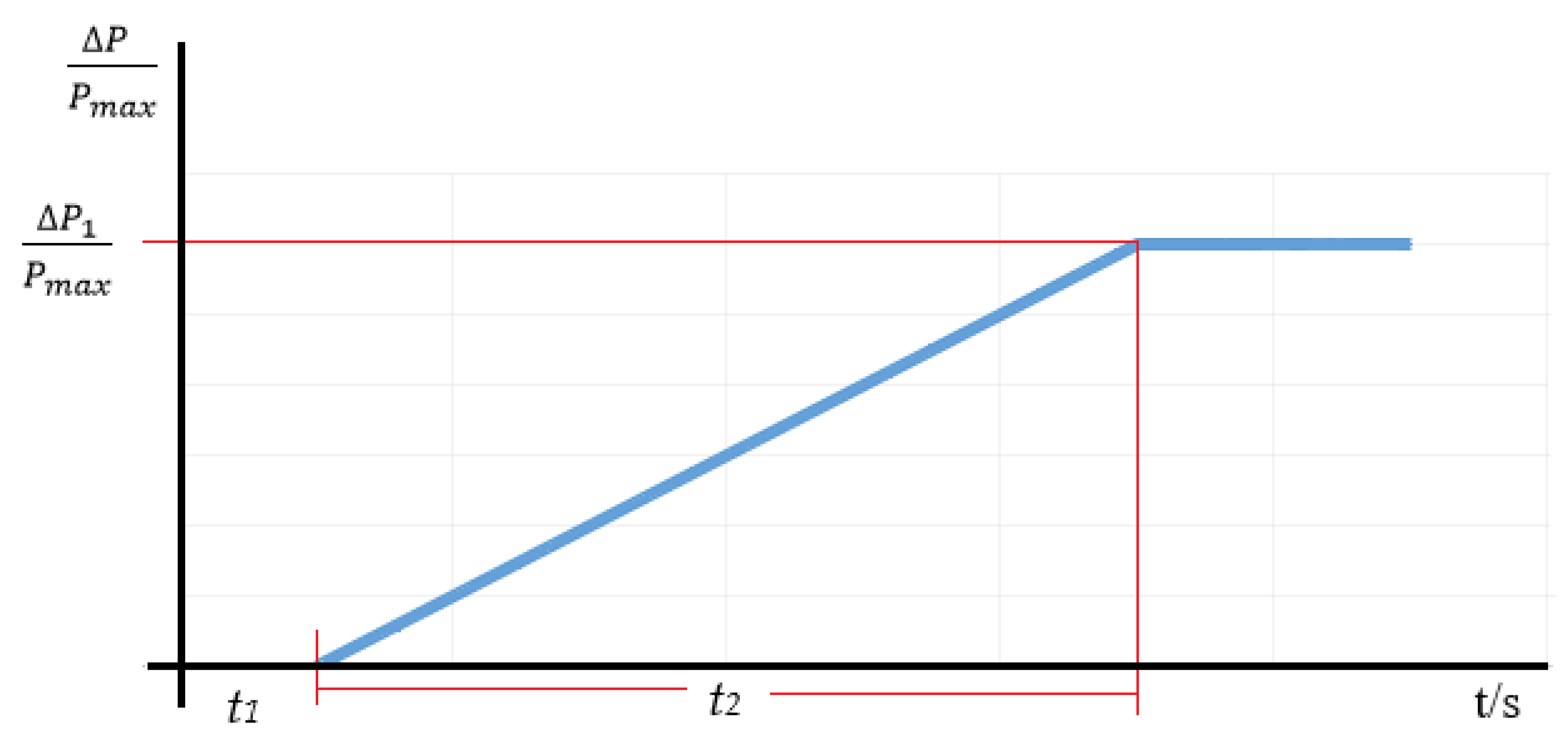
The following are the primary frequency and power reserve requirements that any generators providing the FCR services or that are connected to the transmission system must meet [6] requirements (Figure 1).

Figure 1.
Active power frequency response capability [6].
For the PSHP to provide FCR and FRR services, the PSHP must be able to operate at a partial load and to be able to both quickly and frequently change the operating mode from pump to generator and vice versa. As such, any unstable operating conditions have a negative impact on the entire PSHP system, including on the planned modes of operation for any power operating in a constant state [8]. In [9,10], after considering all potential possibilities for virtual frequency control of PSHP in combination with the examination of the usage of wind farms or diesel generators in islanded operation, it was established that PSHP is too slow to provide FCR.
More details regarding the unstable operation of PSHP under fast-changing and transient load conditions are described in [11,12]. In [11], examining and explaining the influence of the S-shape characteristic on the operation of the PSHP, the authors identified complex flows in the S-shape characteristic zone, such as backflow at the runner inlet, stationary vortex formation, and a rotating stall in the vaneless space. As such, any sudden changes in pressure drop, turbine or generator rotor speed, and torque can be observed in short-term and intermittent operations.
Other authors [13,14,15] examined complementary technologies to balance short-term power fluctuations due to volatile RES production through PSHP. The authors named the disadvantages of PSHP to be slow responses due to high water constants, which occurred as compensation for the need for additional technology to supply and consume power in a relatively short period of time to avoid excessive system-wide power and frequency fluctuations.
Several papers examined the positive impact of PSHP on the provision of short and medium-term regulatory services in an RES dominated power system. According to [16,17,18,19,20], in all studies, PSHP is considered an independent operating unit or one connected to VPPs, and PSHP is modeled using a simplified mathematical model. In doing so, this takes into account capacity; power limits; and in some cases, both the lower and upper permissible power limits, without considering the dynamic capabilities of the PSHP. There is a very limited number of studies that provided detailed and dynamic analyses of PSHP usage and system integration. Many scientists are looking for new ways to balance the increasing number of short-term fluctuations that occur in an actively changing power system, thus eliminating short-term frequency fluctuations and doing so without exceeding the allowable bandwidth of power fluctuations occurring on interconnectors. Therefore, many papers examine and refine an automatic generation control (AGC) algorithms to increase the integration of renewable energies (e.g., solar and wind power) together with hydro power plants (HPPs) or PSHP. Guezgouz [21] proposed an energy management strategy that combines PSHP with a flexible battery system to balance solar and wind farms. The above-proposed management strategy is based on the Gray Wolf optimization method, which aims to optimize such an integrated system by streamlining its composition of it. The author of [22] proposed to combine a battery systems into an AGC system to reduce the impact of RES power fluctuations on the power system. In [23], the authors analyzed the influence of system load fluctuations on frequency regulation when AGC was installed in both thermal–thermal and hydro–thermal environments. To improve system frequency control, this paper proposed simultaneously optimizing the parameters of AGC and Double-Fed Induction Generator (DFIG) controllers using the Cuckoo search algorithm.
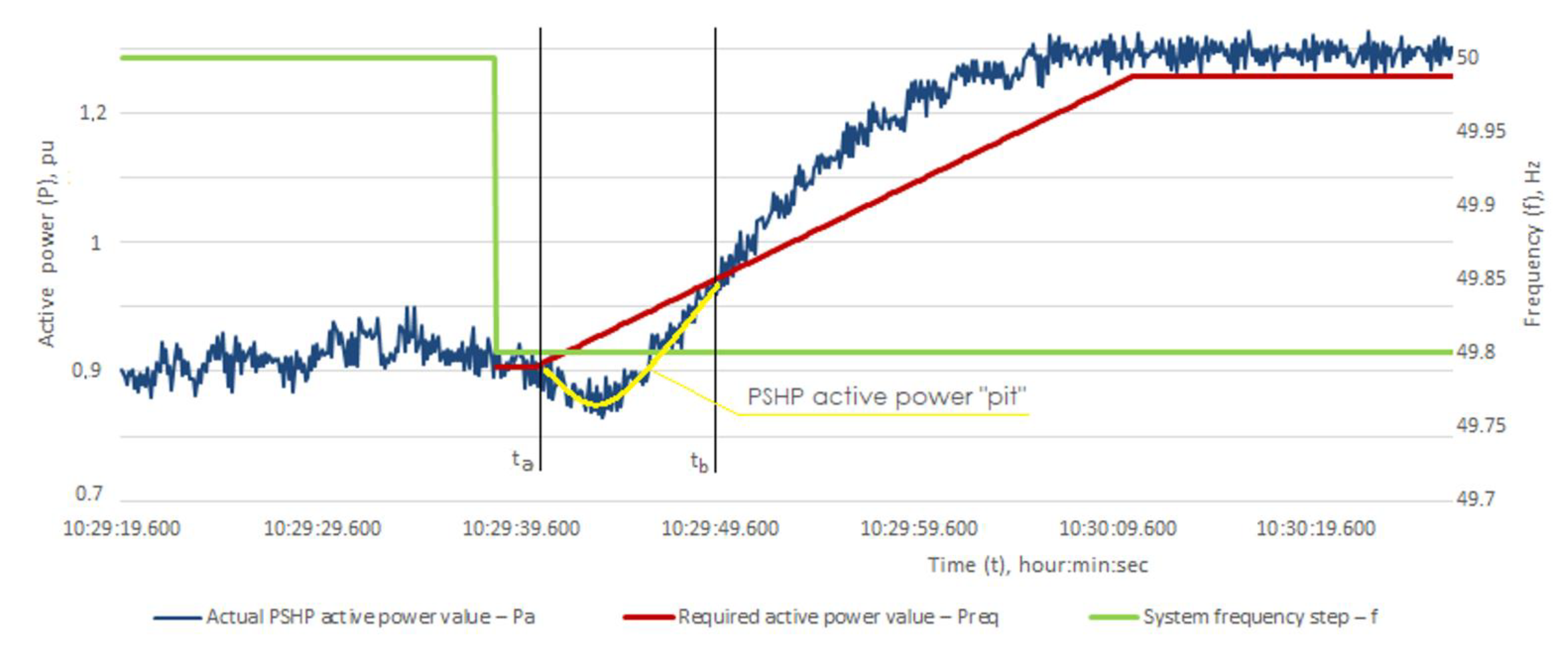
The analyzed papers mentioned above only confirm the results of real measurements (Figure 2), where the regulation of short-term power fluctuations and the provision of FCR services are not possible with the use of PSHP. From the curve in Figure 2, we can see that after activating the FCR, due to a cavitation phenomenon and high water constant observable active power loss only at the initial moment of activation, an increase is observed approximately 6–10 s following. Therefore, PSHP is unable to meet the requirement outlined by network codes [6,7], which requires generators providing FCR service to be able to fully activate power within 2 s to meet the set power increase characteristic from Figure 1, thus limiting their participation in the FCR services provider market.

Figure 2.
Actual curves of the PSHP when primary power regulator is activated.
2.2. BESS Participation in the Ancillary Services Market
More than one paper examined and presented solutions for the use of BESS in short-term power regulation regimes, including the possibility for them to be utilized in FCR. In [24], the authors suggested a possibility for leasing BESS, where the consumer was given the opportunity to increase the profits provided by BESS by combining energy sources as well as by providing frequency management services. Additionally, many papers provided innovative solutions for battery power optimization, the control of various algorithm methods, and successful battery participation in the FCR market [25,26,27,28,29,30]. Due to its fast electrochemical processes, BESS is mainly used to provide ancillary services. Most energy storage technologies are connected to the grid via power converters, so they can change their active power output and consumption over the entire power range in a matter of 0.5–2 s. BESSs with appropriate control systems have the potential to help the power system in reducing frequency deviations better than conventional generators [31].
There are currently no published scientific papers outlining when PSHP is involved in primary frequency regulation. Only [5] provides an instance where the 13 MWh battery is used as ancillary equipment to the existing PSHP, which contributes to energy supply by ensuring FCR, FRR, and RR. A more detailed outline operation of the technology and algorithms is not provided.
This paper presents an algorithm that not only allows PSHP to ensure FCR but also ultimately helps to increase PSHP flexibility and provides the opportunity to work in short-term power control modes. This solution can be used as a remote virtual power plant that can optimize the response of each PSHP governor during a short circuit, thus ensuring the requirements and quality of the FCR as specified in the network code requirements.
3. The Methodology and Mathematical Models
The aims of the methodology development and its effectiveness research include the following:
- Using the results of real measurements of a hydro-generator (PSHP), while FCR is activated, to develop a methodology for determining the transfer function;
- Determining the transfer function suitable for use in real controllers; and
- Checking the suitability of the obtained transfer function for hydro “pit” compensation while the FCR operates.
Hydroelectric electromechanical processes related to active power and frequency control are usually modeled using the following mathematical models: HYGOV, HYGOV2, HYGOVM, HYGOVRU, etc. The simpler mathematical model chosen in this study consists of a single transfer function, the parameters of which are determined using parametric identification. This function is used to model the unit’s characteristics during the initial transition process for up to 6–10 s because, in this power range, hydro units generally do not meet the requirements stated in [6].
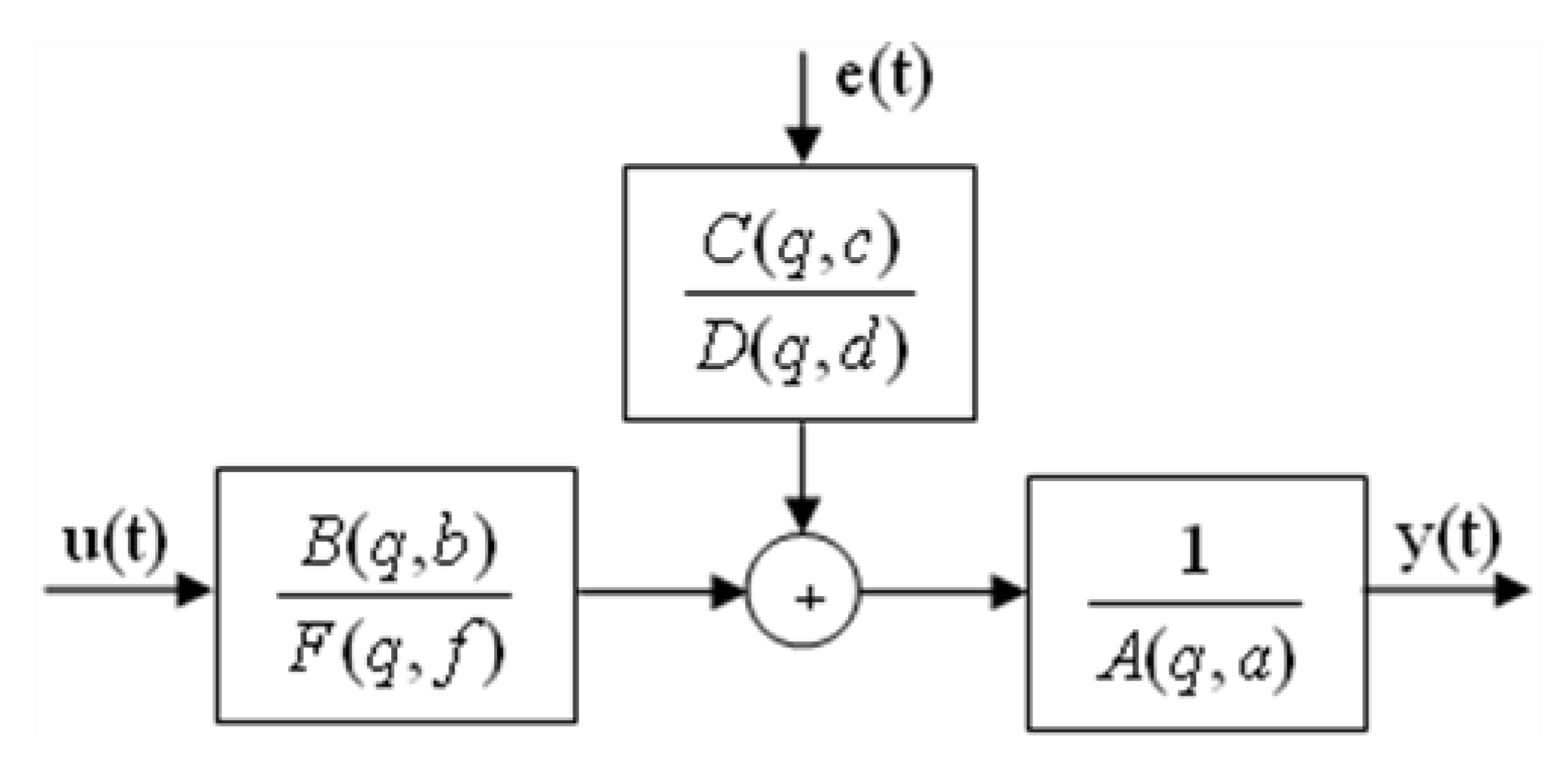
The typical discrete-time linear mathematical model (Figure 3) used for parametric identification can be summarized as follows:

Figure 3.
The schematic diagram of a generalized typical discrete-time linear mathematical model.
Depending on the polynomial combinations of A, B, C, D, and F, there can be thirty-two structures of the mathematical models. In the study, three models were used in parametric identification (autoregressive moving average model with exogenous inputs model (ARMAX), Output Error Model (OE), Box–Jenkins (BJ)). These models were selected to determine the parameters of the mathematical model of the hydro unit (to obtain the best estimates).
3.1. ARMAX Model
ARMAX model structure is as follows:
Accordingly, we have the following:
A simplified expression can be rewritten:
A(q, a)y(t) = B(q, b)u(t − nk) + C(q,c)e(t).
This model is recommended for modeling dynamic systems and autoregressive moving average processes.
3.2. OE Model
The OE model does not use any parameters to model the noise/interference characteristics. The model identifying the parameters of the OE model is the same as the ARMAX model. This is a slightly simpler structure model than the BJ mathematical model and is a separate case of the BJ model. If the component of the real disturbance is close to white noise e(t), then this model can ensure the conditions of identification and achieve high adequacy of the model for real processes.
The OE model is expressed as follows:
Accordingly, we have the following:
nb: B(q) = b1+b2 q−1+⋯+bnb q−nb+1,
nf: F(q) = 1+f1 q−1+⋯+fnf q−nf.
3.3. BJ Model
The BJ polynomial model is more complex than the ARMAX and OE models, and a more complex optimization problem needs to be solved to obtain results. The problem of double model selection has to be solved, i.e., not only the dependence coefficients of the input and output values describing the model but also the parameters of the noise transfer functions are selected. The BJ model is recommended for use in modeling dynamic systems.
The optimized structure of the BJ model can be expressed as follows:
The sequence of the BJ model is defined by the following:
To apply the discrete transfer function to most controllers, a Laplace transform was performed, and continuous transfer function was obtained, but if the controller can implement Z transformation, then it is recommended to use discrete transfer function, avoiding additional errors related to transfer function transformation. The parameters of the mathematical model are selected during the optimization:
After concluding mathematical models, it is very important to evaluate their adequacy in the real system. In this study, identity is assessed by calculating these parameters:
3.4. The Data Used in the Calculations
In 2019–2020, the tests and measurements were performed in the power plants of the Lithuanian electricity system to create mathematical models of the power plants. For the selected PSHP, all measurements, results, and profiles/graphs are not included in the paper to ensure energy security and data confidentiality.
Measurements were performed in the power plant using a test bench. With it, the frequency step signal was transmitted to the power plant control system. Measurement data were captured at all primary active power set points: Pn1 = 0.9 pu and Pn2 = 1 pu, at +200 mHz and −200 mHz frequency deviation. Four curves, Pn1(−200), Pn1(+200), Pn2(−200), and Pn2(+200), were obtained and used for the calculations presented in this paper. The recorded measurements data were further used in the calculations to obtain a transfer function; to compensate for the active power deficit/surplus of the PSHP when FCR is activated; and to provide the FCR according to requirements (graph shown in red in Figure 2) [6]. The measurements provided in Figure 2 were aggregated to obtain a universal transfer function. The four curves obtained during the measurements were aggregated, and three curve stets were derived. It should be noted that the PSHP active power “pit” (yellow curve, Figure 2) was used for the calculations, i.e., part of the curve where the active power of the PSHP reaches the value of the FCR requirement (point of intersection of the red and blue graphs in Figure 2).
3.5. The Developed and Proposed Methodology
- 1.
- The required active power value Preq was calculated to activate FCR, based on FCR requirements (in accordance with the requirements stated in [6]).
- 2.
- Active power difference PΔ was calculated, at t1 = i + tst, for each time period i, between the actual PSHP active power value Pa and the required active power Preq for FCR:For further calculations, the measurement data were used in the time interval, from ta to tb (Figure 2). The active power differences PΔ1(−200), PΔ1(+200), PΔ2(−200), and PΔ2(+200) were calculated for each curve in the range from ti to tb, Pn1(−200), Pn1(+200), Pn2(−200), Pn2(+200).
- 3.
- Measurement data were aggregated and obtained three different measurement data sets (hereinafter “Measurements”):
- 3.1
- First Measurements: maximum value PΔ1(−200), PΔ1(+200), PΔ2(−200), and PΔ2(+200) in the range (ta; tb). That means the maximum value from four real measured curves was used to compile a new curve;
- 3.2
- Second Measurements: one of four curves was selected, taking into account the maximum deviation of PΔ1(−200), PΔ1(+200), PΔ2(−200), and PΔ2(+200) curves by amplitude in the range (ti; tb).
- 3.3
- Third Measurements: the arithmetic mean of four curves was calculated:
- 4.
- New value is calculated when the aggregated curve of each Measurement is moved upward so that the active power crosses zero value at time ta when FCR is activated. Therefore, the initial value of active power at time ta is subtracted from all values of active power up to tb so that the initial value of PΔ starts from zero (Figure 4):
 Figure 4. Representation of the PSHP transition process.
 - 5.
- Parametric identification was performed using the aggregated Measurements obtained in the fourth point of the methodology. Three sets of discrete transfer functions for each Measurement were obtained using the BJ, ARMAX, and OE parametric identification models. Transfer functions for the first set are presented below. The transfer function in (22) was obtained by the OE model, that of (23) was obtained by ARMAX, and that of (24) was obtained by BJ. The other two sets of transfer functions are not presented in this paper.
- 6.
- Ryŷ and R2 coefficients were calculated for all three sets of transfer functions to choose the most accurate transfer function. The calculation results are presented in Table 1.
 Table 1. Ryŷ coefficient of discrete transfer functions.
 - 7.
- The continuous transfer functions are derived from the discrete transfer function (first sets—(22)–(24); second and third sets not presented in the paper) using Laplace transform. Such a transform is performed to facilitate implementation of the controller algorithm in practice, as most controllers support continuous transfer functions, and moreover, it simplifies the tuning work of controllers, as continuous transfer functions are engineer-friendly (engineers usually have more experience with continuous transfer functions). The continuous transfer function in (25) was obtained by the OE model, that of (26) was obtained by ARMAX, and that of (27) was obtained by BJ.Other sets (second and third) of transfer functions were obtained using the same method.
- 8.
- The most accurate transfer functions that were obtained by the OE parametric identification model were selected based on the Ryŷ and R2 calculated in the sixth point of the methodology. As we see from the results presented in Table 1, the OE parametric identification model is 2.31% more accurate than ARMAX and 4.04% more accurate than BJ. The transfer functions in (28)–(30) obtained by the OE model have the highest Ryŷ (0.908). These transfer functions are used in further calculations. It is worth mentioning that (28) obtained by the OE model using first Measurements are a maximum value (3.1), that (29) obtained using the second Measurements are the maximum deviation (3.2), and that (30) obtained using the third Measurements are the arithmetic mean (3.3).
- 9.
- To be able to achieve optimal performance of BESS covering active power “pit”, it is necessary to calculate proper sizing of the battery. In general, BESS capacity (MWh) is calculated by using Equation (31):Therefore, with real measurement data of the PSHP, more accurate mathematical equations are used (Equation (32)). It requires accurate measurements with a high sampling rate.The simplified Equation (33) presents how to calculate BESS capacity (MWh) in a more convenient way if real measurements of PSHP are known:The BEES power in MW can be calculated using the maximum value between Pa and Preq in time periods ta and tb of the real data measurements of PSHP presented in Figure 4:
4. Results and Discussion
The continuous low-order transfer functions are easier to adapt and configure controllers. These transfer functions require the frequency change input signal to obtain the active power difference at the controller output and to submit a command to the battery system.
In this paper, the frequency change signal is simulated and submitted as an input signal of transfer functions; therefore, the active power is obtained at the output. It is important to mention that the output curve of transfer function is used for the first 6–10 s only to compensate for the power deficit/surplus of the PSHP and to meet the requirements of the FCR requirements stated in [6]. Depending on the water time constant of the HPSPP and hydraulic processes in the hydro turbine, the time period of power surplus/deficit (the first few seconds when FCR activated) may vary. Therefore, the transfer function is adjusted for each HPSPP or HPP using provided methodology in Section 3.5. considering the results of real measurements when FCR is activated.
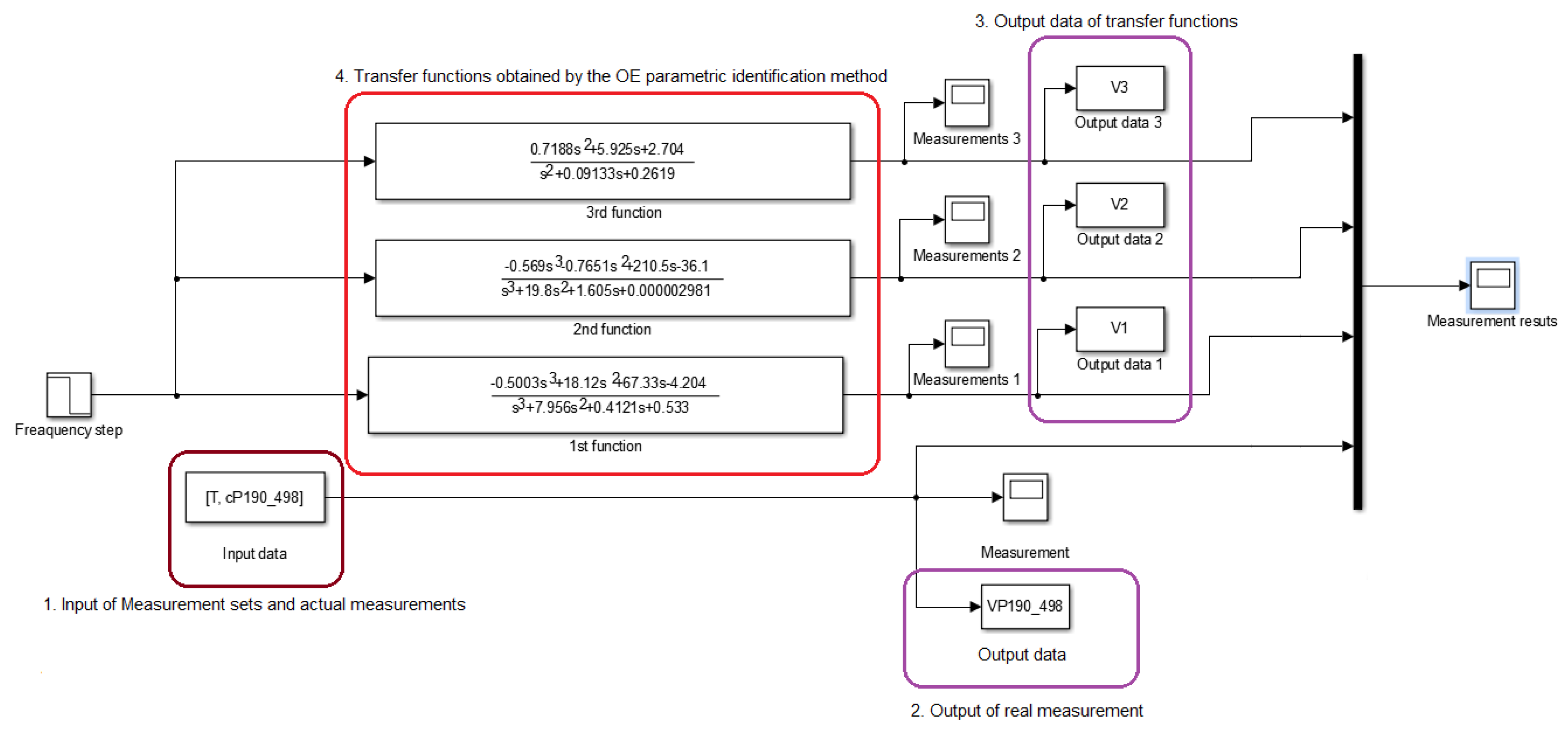
A calculation in the Matlab Simulink environment was performed to investigate the efficiency of the developed methodology. The simulated frequency step is an input signal of the transfer functions in (28)–(30) in the MATLAB Simulink environment (Figure 5).

Figure 5.
Research model developed in the Simulink environment.
The output signals of the transfer functions in (28)–(30) obtained by the OE parametric identification model at the frequency change (fourth square, Figure 5) are compared with the actual measurement data Pn1(−200), Pn1(+200), Pn2(−200), and Pn2(+200) and aggregated measurements (first square, Figure 5) obtained according to Section 3.5, (3.1, 3.2, and 3.3 points) (Figure 6).

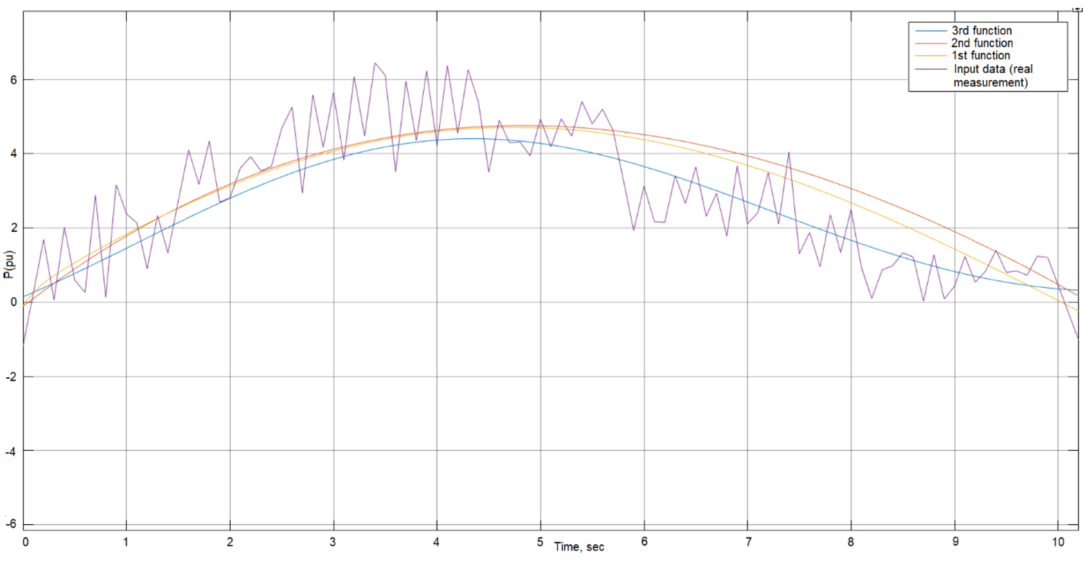
Figure 6.
Comparing the real measurement Pn1(−200) and the functions in (28)–(30), when the frequency deviates by −200 mHz.
The output data of research model (Figure 5) in square No. 2 “Real measurement output” and No. 3 “Output of the transfer functions” were used to calculate the Ryŷ, RMSE, and R2 coefficients. Real-time measurements (Pn1(−200), Pn1(+200), Pn2(−200), Pn2(+200)) and transfer functions (28)–(30) were used. The calculated results are presented in Table 2.
Table 2.
Ryŷ, RMSE, and R2 coefficients of continuous transfer functions obtained by the OE model, when actual measurements, at ± 200 mHz frequency deviation (Pn1(−200), Pn1(+200), Pn2(−200), Pn2(+200)), were used.
As we can see from Table 2, output signal of the transfer function (30) has the most accurate results in comparison with actual measurements because Ryŷ is the highest and RMSE is the smallest. From the Ryŷ results, we see that the output signal of transfer function (30) is 2.31% better than that of transfer function (28) and 1% better than that of transfer function (29). The same is seen for the R2 results in that the output signal of transfer function (30) is 4.77% better than that of transfer function (28) and 2.00% better than that of transfer function (29). RMSE proves that the output signal of transfer function (30) shows the best results—25.23% and 45.87% accordingly.
Ryŷ, RMSE, and R2 were calculated in the same way as that for the data provided in Table 2. Instead, real-time measurements (Pn1(−200), Pn1(+200), Pn2(−200), Pn2(+200)) used aggregated Measurement (3.1, 3.2, and 3.3). The calculated results are presented in Table 3.
Table 3.
Ryŷ, RMSE, and R2 coefficients of continuous transfer functions obtained by the OE model, when aggregated Measurements (3.1, 3.2, and 3.3) were used.
As we see from the calculation results provided in Table 3, it is obvious that the third function shows the most reliable results by covering the “pit” of the PSHP when FCR is activated because Ryŷ is the highest coefficient and the RMSE is the lowest. From the Ryŷ results, we see that the output signal of transfer function (30) is 3.32% better than that of transfer function (28) and 4.36% better than that of transfer function (29). Similarly, the R2 results show that the output signal of transfer function (30) is 6.54% better than that of transfer function (28) and 8.53% better than that of transfer function (29). RMSE proves that the output signal of transfer function (30) shows the best results—143.48% and 160.75% accordingly. Moreover, transfer function (30) has the smallest order, which leads to a mathematically more stable state.
Seeing as aggregated measurements were used to obtain transfer functions, calculation results in Table 3 are better because function output results are compared with the same aggregated measures. To determine which function to use in a real system, it is necessary to consider the results of Table 2, as the output signal of the function is compared with the actual measurements. This gives the most precise picture of transfer function capability to cope with the hydro-generator “pit” and to supply/consume a necessary amount of active power in case of PSHP participating in the FCR market.
The comparison of the results was performed according to Ryŷ, as this coefficient shows exactly how the output signal of the function corresponds to the trend of the compared curve and not to the active power peaks, as RMSE indicates. In a real system, it is most important to follow the PSHP/HPP active power decrease/increase trend, as it impacts system stability. The power system inertia will “cut out” the active power peaks and therefore will be not visible in a real system, so it is meaningless to follow the active power peaks.
5. Validation of Transfer Function Modeling BESS
BESS model with an embedded transfer function (29) simulated in Simulink consists of a 3.6 MWh and a 9 MW Li-ion battery. Capacity (MWh) and power (MW) were calculated using Equations (33) and (34) accordingly. It is recommended that the transmission or distribution system operators determine the j coefficient (33) and issue as one of the mandatory requirements in the connection condition to connect BESS to a power system.
In this paper, the j coefficient was calculated by assuming that FCR services are provided only up to one hour because such a mode is the most difficult for BESS operation. It is worth mentioning that FCR services are usually provided both upward and downward throughout an hour in a real system. The quantity of FCR services, provided both downward and upward throughout the hour, is approximately equal. To accurately determine the value of j, the historical data of the frequency measurements must be evaluated; therefore, statistical analysis must be performed.
The controller activates BESS at the initial time period simultaneously with FCR, when the frequency of the power system deviates from the nominal value. The total activating time of BESS is calculated as follows:
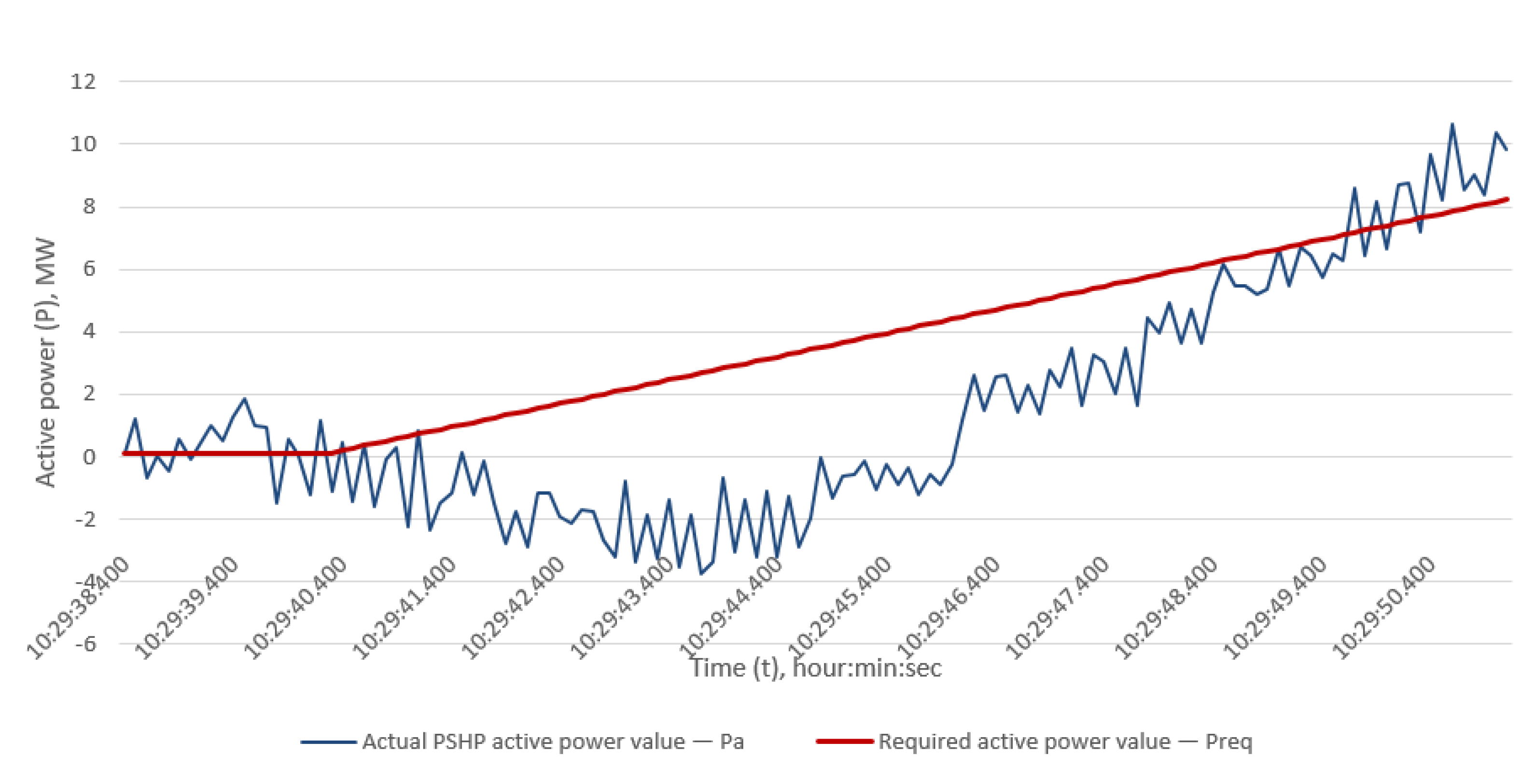
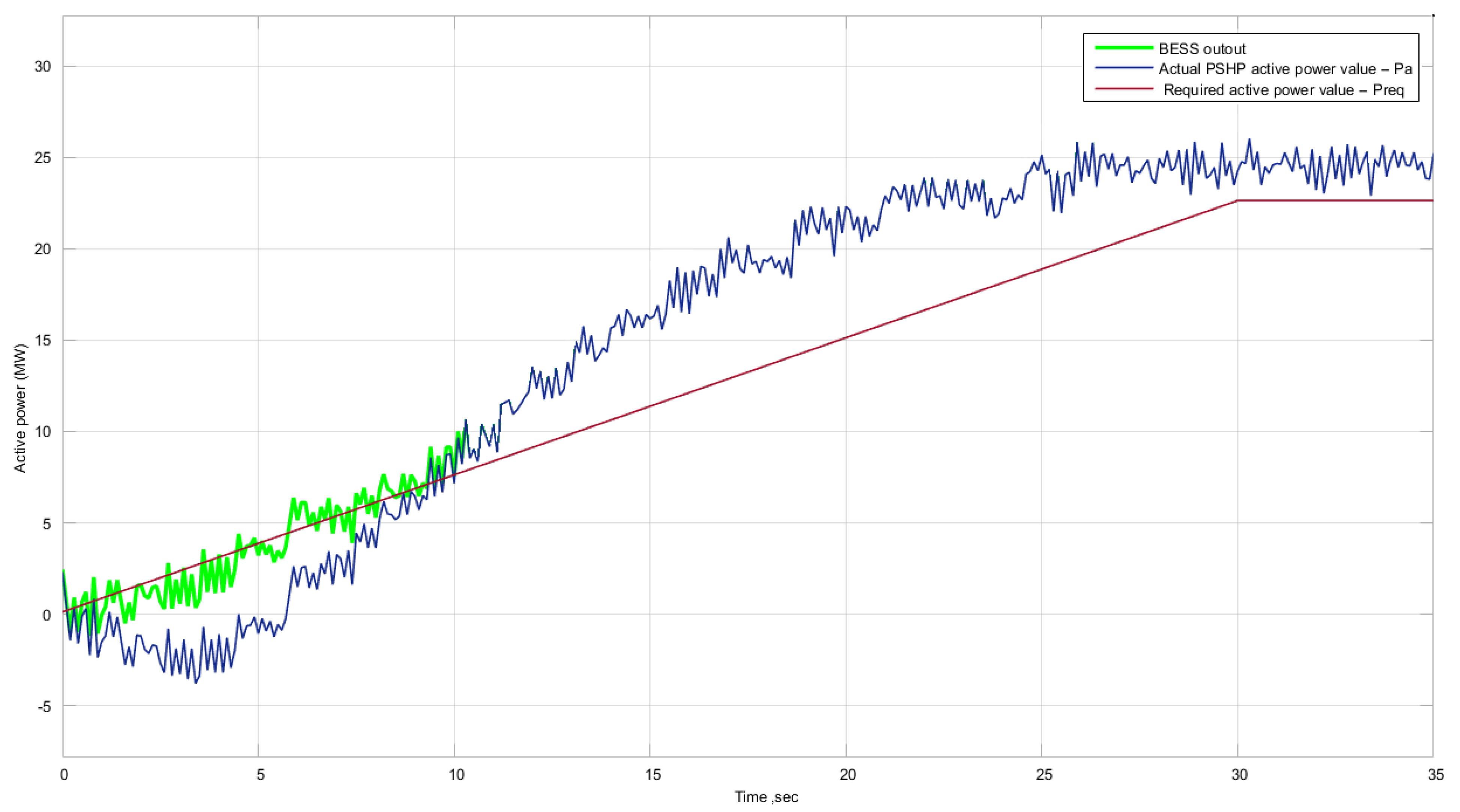
In a Li-ion battery, the maximum active power can be activated within 0.5–1 s, and the maximum ramping speed is 0.021–0.042 MW/ms. According to Figure 7, the maximum power shall be activated at the fourth second. After analyzing real data measurements, it can be concluded that BESS shall reach maximum active power output between the fourth and sixth second (measurements cannot be enclosed in the paper due to confidentiality).

Figure 7.
Comparison of BESS output (green) and actual PSHP output activating FCR with required active power output.
The results show that BESS with an embedded transfer function (29) improves the active power input to the power system and covers the PSHP active power “pit”. The results provided in Figure 7 prove that the derived transfer function using the provided methodology allows PSHP to provide FCR services according to the requirements stated in [6].
6. Conclusions
A methodology was developed to obtain a transfer function using PSHP measurement data recorded during a real experiment when FCR is activated. The continuous low-order transfer functions created using the Laplace transform can be applied and used in real controllers.
Parametric identification mathematical models (ARMAX, OE, BJ) were used to obtain transfer functions. The most optimal OE identification model was selected because it is 2.31% more accurate than ARMAX and 4.04% more accurate than BJ, and discrete, continuous transfer functions were created.
The output signal of continuous transfer functions was compared with actual and aggregated measurements. The correlation function (), determination coefficient (R2), and root-mean-square error (RMSE) were calculated to determine which transfer function is capable of coping with a hydro-generator “pit” and to supply/consume a necessary amount of active power in case PSHP participates in the FCR market.
The correlation results in Table 2 show that, when comparing transfer functions’ output signals with the actual measurements, the output signal in transfer function (30) is 2.31% better than that of transfer function (28) and 1% better than that of transfer function (29). Comparing the output signals from transfer functions with aggregated measures shows that the output signal of transfer function (30) is 3.32% better than that of transfer function (28) and 4.36% better than that of transfer function (29). Based on the calculation results, using the transfer function in (30) in a real system was suggested. Moreover, this function has the smallest order, so its output signal is closer to the active power trend of PSHP curve, and such a function is mathematically more stable.
It can be concluded that using the provided methodology and obtained transfer function in combination with BESS allows PSHP to provide FCR services according to the requirements stated in [6]. This transfer function is based on the power system frequency deviation signal, which is transmitted to the input of the transfer function, and its output signal is the active power order to BESS. This output signal is used only at the initial time until the PSHP reaches the value of the active power required by regulations to participate in FCR services; in other words, BESS only operates in the range of active power variation in which PSHP does not meet the requirements of [6].
A methodology for battery power (MW) and capacity (MWh) selection is proposed. The proposed transfer function allows for combining battery systems with HPP/PSHP to VPP. The biggest benefit of such a VPP is not only providing FFR and RR services but also allowing participation in the market of FCR provision services. Taking into account the increasing integration of RES and the fact that many European countries have a goal to reach 100% generation of electricity from RES, the proposed methodology allows for obtaining a transfer function for BESS, which in combination with HPP/PSHP, can be successfully integrated into the market of ancillary services as remote VPP.
Author Contributions
Conceptualization, P.C. and V.R.; methodology, P.C.; software, P.C.; validation, P.C. and V.R.; formal analysis, P.C.; writing—original draft preparation, P.C.; writing—review and editing, P.C. and V.R.; visualization, P.C.; supervision, V.R. All authors have read and agreed to the published version of the manuscript.
Funding
This research received no external funding.
Institutional Review Board Statement
Not applicable.
Informed Consent Statement
Not applicable.
Data Availability Statement
Not applicable.
Conflicts of Interest
The authors declare no conflict of interest.
Nomenclature
| the active power range and the maximum power ratio (frequency response range); | |
| t1 | the maximum allowable initial delay, up to 2 s; |
| t2 | the maximum allowed activation time, up to 30 s; |
| A, B, C, D, F | polynomial functions; |
| q | the time shift operator; |
| u(t) | freely variable input variable (e.g., control signal); |
| y(t) | output variable; |
| e(t) | sequence of unrelated random values, also called white noise; |
| a, b, c, d, f | vectors of parameters of corresponding polynomials; |
| y(t) | output at time t; |
| u(t) | input at time t; |
| na | the order of the autoregressive (AR) model; |
| nb | the order of the exogenous input model (X); |
| nc | the order of the moving average model (MA) |
| nk | number of input samples; |
| y(t−1)…y(t−na) | primary outputs; |
| u(t−nk)…u(t−nk− nb+1) | primary and delayed inputs; |
| e(t−1)…e(t−nc) | white noise value; |
| the parameter vector; | |
| na, nb, nc | coefficients of ARMAX model variables; |
| nk | a delay of ARMAX; |
| q | the backward shift operator of ARMAX; |
| correlation function; | |
| actual/measured value; | |
| y(t) | value of the parameter of ; |
| R2 | determination coefficient; |
| RMSE | root-mean-square error; |
| tst | FCR activation delay, which is determined for each HPP individually; |
| n | sampling of measurement data (measurement time step); |
| P | active power, pu; |
| f | frequency, mHz; |
| the capacity, MWh; | |
| t | time period for capacity calculation, sec; |
| P | active power, MW; |
| needed BESS capacity, MWh; | |
| required capacity, MWh; | |
| BESS actual capacity, MWh; | |
| ta, tb | time period for the calculation of needed BESS capacity (duration of PSHP active power “pit”), sec; |
| required active power according to [6], MW; | |
| the actual power output of PSHP, MW; | |
| k | battery activation time in hours, depending on characteristics of PSHP generator; |
| j | battery activation quantity providing FRC services, times per hour; |
| needed BESS power, MW; | |
| coefficient of battery depth of discharge, pu; | |
| coefficient of battery efficiency, pu; | |
| BESS total activating time, sec. |
References
- Aziz, A.; Than Oo, A.; Stojcevski, A. Analysis of frequency sensitive wind plant penetration effect on load frequency control of hybrid power system. Int. J. Electr. Power Energy Syst. 2018, 99, 603–617. [Google Scholar] [CrossRef]
- Chen, M.; Xiao, X. Hierarchical frequency control strategy of hybrid droop/VSG-based islanded microgrids. Electr. Power Syst. Res. 2018, 155, 131–143. [Google Scholar] [CrossRef]
- Gerdun, P.; Ahmed, N.; Weber, H. Active Power Regulation of a Storage Power Plant (SPP) with Voltage Angle Control as Ancillary Service. IFAC-PapersOnLine 2020, 53, 13477–13482. [Google Scholar] [CrossRef]
- Liu, J.; Chen, X.; Cao, S.; Yang, H. Overview on hybrid solar photovoltaic-electrical energy storage technologies for power supply to buildings. Energy Convers. Manag. 2019, 187, 103–121. [Google Scholar] [CrossRef]
- Schreider, A.; Bucher, R. An auspicious combination: Fast-ramping battery energy storage and high-capacity pumped hydro. Energy Procedia 2018, 155, 156–164. [Google Scholar] [CrossRef]
- Commission Regulation (EU) 2016/631, Network Code on Requirements for Grid Connection of Generators. Available online: https://eur-lex.europa.eu/eli/reg/2016/631/oj (accessed on 14 April 2016).
- Commission Regulation (EU) 2017/1485, Guideline on Electricity Transmission System Operation, 2 August 2017. Available online: https://eur-lex.europa.eu/legal-content/EN/TXT/?uri=uriserv:OJ.L_.2017.220.01.0001.01.ENG (accessed on 2 August 2017).
- Cavazzini, G.; Houdeline, J.-B.; Pavesi, G.; Teller, O.; Ardizzon, G. Unstable behaviour of pump-turbines and its effects on power regulation capacity of pumped-hydro energy storage plants. Renew. Sustain. Energy Rev. 2018, 94, 399–409. [Google Scholar] [CrossRef]
- Papaefthymiou, S.V.; Lakiotis, V.G.; Margaris, I.D.; Papathanassiou, S.A. Dynamic analysis of island systems with wind-pumped-storage hybrid power stations. Renew. Energy 2015, 74, 544–554. [Google Scholar] [CrossRef]
- Martínez-Lucas, G.; Sarasúa, J.I.; Sánchez-Fernández, J.Á. Eigen analysis of wind–hydro joint frequency regulation in an isolated power system. Int. J. Electr. Power Energy Syst. 2018, 103, 511–524. [Google Scholar] [CrossRef]
- Zuo, Z.; Fan, H.; Liu, S.; Wu, Y. S-shaped characteristics on the performance curves of pump-turbines in turbine mode—A review. Renew. Sustain. Energy Rev. 2016, 60, 836–851. [Google Scholar] [CrossRef]
- Fu, L.; Wei, J.; Huang, B. Research on influence factors of primary frequency regulation contribution electric energy of hydropower unit. In Proceedings of the 2019 IEEE 3rd Conference on Energy Internet and Energy System Integration (EI2), Changsha, China, 8–10 November 2019; Volume 3, pp. 1058–1063. [Google Scholar]
- Zhao, H.; Wu, Q.; Hu, S.; Xu, H.; Nygaard Rasmussen, C. Review of energy storage system for wind power integration support. Appl. Energy 2015, 137, 545–553. [Google Scholar] [CrossRef]
- Brown, P.; Lopes, J.A.; Matos, M. Optimization of Pumped Storage Capacity in an Isolated Power System with Large Renewable Penetration. IEEE Trans. Power Syst. 2008, 23, 523–531. [Google Scholar] [CrossRef]
- Makarov, Y.V.; Yang, B.; DeSteese, J.G.; Lu, S.; Miller, C.H.; Nyeng, P.; Ma, J.; Hammerstrom, D.J.; Vishwanathan, V.V. Wide-Area Energy Storage and Management System to Balance Intermittent Resources in the Bonneville Power Administration and California ISO Control Areas; Pacific Northwest National Laboratory (PNNL): Richland, WA, USA, 2008. [Google Scholar]
- Nathaniel, S.; Pearre, L.; Swan, G. Technoeconomic feasibility of grid storage: Mapping electrical services and energy storage technologies. Appl. Energy 2015, 137, 501–510. [Google Scholar]
- Bradbury, K.; Pratson, L.; Patiño-Echeverri, D. Economic viability of energy storage systems based on price arbitrage potential in real-time U.S. electricity markets. Appl. Energy 2014, 114, 512–519. [Google Scholar] [CrossRef]
- Deane, J.P.; Gallachóir, B.P.Ó.; McKeogh, E.J. Techno-economic review of existing and new pumped hydro energy storage plant. Renew. Sustain. Energy Rev. 2010, 14, 1293–1302. [Google Scholar] [CrossRef]
- Pérez-Díaz, J.I.; Jiménez, J. Contribution of a pumped-storage hydropower plant to reduce the scheduling costs of an isolated power system with high wind power penetration. Energy 2016, 109, 92–104. [Google Scholar] [CrossRef] [Green Version]
- Cavazzini, G.; Pavesi, G.; Ardizzon, G. A novel two-swarm based PSO search strategy for optimal short-term hydro-thermal generation scheduling. Energy Convers. Manag. 2018, 164, 460–481. [Google Scholar] [CrossRef]
- Guezgouz, M.; Jurasz, J.; Bekkouche, B.; Ma, T.; Shahzad Javed, M.; Kies, A. Optimal hybrid pumped hydro-battery storage scheme for off-grid renewable energy systems. Energy Convers. Manag. 2019, 199, 112046. [Google Scholar] [CrossRef]
- Zhao, X.; He, J.; He, L.; Xu, G. A System Compensation Based Model Predictive AGC Method for Multiarea Interconnected Power Systems with High Penetration of PV System and Random Time Delay between Different Areas. Math. Probl. Eng. 2018, 2018, 1–10. [Google Scholar] [CrossRef] [Green Version]
- Chaine, S.; Tripathy, M. Performance of CSA optimized controllers of DFIGs and AGC to improve frequency regulation of a wind integrated hydrothermal power system. Alex. Eng. J. 2019, 58, 579–590. [Google Scholar] [CrossRef]
- Sun, L.; Qiu, J.; Han, X.; Yin, X.; Dong, Z. Per-use-share rental strategy of distributed BESS in joint energy and frequency control ancillary services markets. Appl. Energy 2020, 277, 115589. [Google Scholar] [CrossRef]
- Wu, Y.-K.; Tang, K.-T. Frequency Support by BESS—Review and Analysis. Energy Procedia 2019, 156, 187–191. [Google Scholar] [CrossRef]
- Zhao, T.; Parisio, A.; Milanović, J.V. Location-dependent distributed control of battery energy storage systems for fast frequency response. Int. J. Electr. Power Energy Syst. 2021, 125, 106493. [Google Scholar] [CrossRef]
- Yuan, Z.; Wang, W.; Wang, H.; Yıldızbaşı, A. Allocation and sizing of battery energy storage system for primary frequency control based on bio-inspired methods: A case study. Int. J. Hydrog. Energy 2020, 45, 19455–19464. [Google Scholar] [CrossRef]
- El-Bidairi, K.S.; Nguyen, H.D.; Thair, S.; Mahmoud, S.D.G.; Jayasinghe, J.; Guerrero, M. Optimal sizing of Battery Energy Storage Systems for dynamic frequency control in an islanded microgrid: A case study of Flinders Island, Australia. Energy 2020, 195, 117059. [Google Scholar] [CrossRef]
- Zecchino, A.; Yuan, Z.; Sossan, F.; Cherkaoui, R.; Paolone, M. Optimal provision of concurrent primary frequency and local voltage control from a BESS considering variable capability curves: Modelling and experimental assessment. Electr. Power Syst. Res. 2021, 190, 106643. [Google Scholar] [CrossRef]
- Tan, Z.; Li, X.; He, L.; Li, Y.; Huang, J. Primary frequency control with BESS considering adaptive SoC recovery. Int. J. Electr. Power Energy Syst. 2020, 117, 105588. [Google Scholar] [CrossRef]
- Fernández-Muñoz, D.; Pérez-Díaz, J.I.; Guisández, I.; Chazarra, M.; Fernández-Espina, A. Fast frequency control ancillary services: An international review. Renew. Sustain. Energy Rev. 2020, 120, 109662. [Google Scholar] [CrossRef]
Publisher’s Note: MDPI stays neutral with regard to jurisdictional claims in published maps and institutional affiliations. |
© 2022 by the authors. Licensee MDPI, Basel, Switzerland. This article is an open access article distributed under the terms and conditions of the Creative Commons Attribution (CC BY) license (https://creativecommons.org/licenses/by/4.0/).