Article

Modified Levy-based Particle Swarm Optimization (MLPSO) with Boost Converter for Local and Global Point Tracking

by
Chanuri Charin
1,2,*,
Dahaman Ishak
1,
Muhammad Ammirrul Atiqi Mohd Zainuri
3,*,
Baharuddin Ismail
2,
Turki Alsuwian
4,* and
Adam R. H. Alhawari
4,*
1
School of Electrical and Electronic Engineering, Universiti Sains Malaysia, Pulau Pinang 14300, Malaysia
2
Faculty of Electrical Engineering and Technology, Universiti Malaysia Perlis, Perlis 02600, Malaysia
3
Department of Electrical, Electronic and Systems Engineering, Faculty of Engineering and Built Environment, Universiti Kebangsaan Malaysia, Selangor 43600, Malaysia
4
Electrical Engineering Department, College of Engineering, Najran University, Najran 11001, Saudi Arabia
*
Authors to whom correspondence should be addressed.
Energies 2022, 15(19), 7370; https://doi.org/10.3390/en15197370
Submission received: 13 July 2022 / Revised: 21 September 2022 / Accepted: 30 September 2022 / Published: 7 October 2022

Abstract

:
This paper presents a modified Levy particle swarm optimization (MLPSO) to improve the capability of maximum power point tracking (MPPT) under various partial shading conditions. This method is aimed primarily at resolving the tendency to trap at the local optimum particularly during shading conditions. By applying a Levy search to the particle swarm optimization (PSO), the randomness of the step size is not limited to a specific value, allowing for full exploration throughout the power-voltage (P-V) curve. Therefore, the problem such as immature convergence or being trapped at a local maximum power point can be avoided. The proposed method comes with great advantages in terms of consistent solutions over various environmental changes with a small number of particles. To verify the effectiveness of the proposed idea, the algorithm was tested on a boost converter of a photovoltaic (PV) energy system. Both simulation and experimental results showed that the proposed algorithm has a high efficiency and fast-tracking speed compared to the conventional HC and PSO algorithm under various shading conditions. Based on the results, it was found that the proposed algorithm successfully converges most rapidly to the global maximum power point (GMPP) and that the tracking of GMPP under complex partial shading is guaranteed. Furthermore, the average efficiency for all test conditions was 99% with a tracking speed of 1.5 s to 3.0 s and an average output steady-state oscillation of 0.89%.

1. Introduction

Considering the depletion of fossil fuels, the role of renewable energy sources is now seen as vital in shaping a more sustainable future. Photovoltaic (PV) energy has attracted considerable attention from both researchers and the industry as an alternative to the conventional fossil fuel-based electricity generation, due to lower manufacturing costs and higher efficiency [1,2]. High-efficiency operation is the major concern regarding the PV system, as energy generated from the PV array should always operate at optimum power in any conditions. The ability to harvest the full amount of energy would help to maximize the return of investment of PV installation [3].
However, the challenge lies in the non-linear characteristics of PV, where the performance depends on the dynamic environmental conditions, i.e., irradiance and temperature. Consequently, the optimum power of the PV system should be extracted with the use of a power electronics converter [4,5]. In response to this, a dc-dc converter is integrated with a maximum power point tracking (MPPT) control to harvest the PV optimum power. As a result, various studies based on maximum power point tracking (MPPT) algorithms have been carried out [6,7]. The most popular techniques, such as perturb and observe (P&O) [8,9,10] and incremental conductance (IC) [11], are widely used in academia and practical applications [12].
Generally, the shading phenomenon is unavoidable in PV generation [10,13]. The shadows of buildings, trees, and clouds lead to a non-uniform irradiance penetrating the PV array [13,14]. Once partial shading occurs, the conventional MPPT control is unable to distinguish the accurate operating point of the PV system [11,13,15]. This idea has gained significant interest in addressing the these disadvantages. The implementation of the hardware method, which increases the complexity and cost of the PV installation, is also explored, but will not be discussed here [1,16]. The antiparallel bypass diode method is, therefore, the simplest solution to prevent the creation of a hot spot due to reverse currents flowing through the cell. This happens once the serially connected cell is in a reversed biased state that may cause heat dissipation in the cell. Dissipated heat can become severe if it is higher than the cell’s maximum power, potentially destroying the cell and causing the device to have an open circuit. Furthermore, the presence of the antiparallel diode creates multiple peaks in the P-V and I-V curves, where the global maximum power point (GMPP) is the highest peak [11]. The rests of the peak are known as the local maximum power point (LMPP) [1,17].
Recently, studies have addressed the problem of partial shading conditions (PSC) in the PV system. Conventional MPPT techniques, such as perturb and observe (P&O) [8,18] and incremental conductance (IC) [19], fail to search for the optimum point [16,20]. In the conventional method, the decision is made based on the gradient of the curve. It uses a fixed step size in the search with an easier climbing process towards the optimum point. A larger step size leads to a faster time to reach the optimum point, but comes with a high probability of overlooking the optimum point. Meanwhile, a small step size in the execution leads to a longer time to reach the optimum point, with lower chances to overlook the optimum point. In the conventional method, the next movement is based on the previous location, and no memory is employed; thus this method fails to identify the optimum point under shading conditions [20,21]. Therefore, soft computing techniques using particle swarm optimization (PSO) [17,18], cuckoo search [22] differential evaluation (DE) [23,24], fuzzy logic control [25], ant colony optimization (ACO) [26], artificial bee colony (ABC) [21,27], musical chairs algorithm [28], salp swarm algorithm (SSA) [29,30,31], horse herd optimization algorithm [13], and the grasshopper optimization algorithm (GOA) [32] are used in the search for the global point. These techniques are more preferable due to their superiority in handling extreme conditions, such as shading and the dynamic change of irradiance [33]. However, the challenge is to choose the right parameters, including initial state, control parameters, population sizes, and the acceptable search space [34]. Mainly, the improper selection of the initial condition causes the convergence to fail at a certain value of power [27,34].
For example, the PSO algorithm, in which this method has intermittent performance under the shading condition. In PSO, the randomness selections of the initial value reduce the efficiency of searching significantly [35,36]. The small perturbation during the exploration process may lead to failure as the operating point is too far from the optimum value. Consequently, more iteration is required for the particle to reach the optimum point. On the other hand, if the perturbation is set too large, it might cause the search to overlook the optimum point and get trapped at a local point. Therefore, by increasing the number of particles, the chances to converge to a feasible solution would be higher [36,37]. However, this can only be performed at some period. If the time needed to track the optimum point is too long, the algorithm might not be practical to be implemented [4,38]. In the next subsection, a review of the algorithm inspired by swarm-based is presented.
Review on Swarm-Based Algorithm
Particle swarm optimization (PSO) is among the leading MPPT techniques used in MPPT applications [18,23]. Figure 1 shows the flowchart of conventional PSO in the MPPT application. The great advantage of the PSO technique is that, once all the particles have reached the MPP, the velocity for all the particles becomes zero. This significantly allows zero steady-state oscillation once convergence is reached [15]. This significantly reduces energy losses and improves the efficiency of the system. Another advantage of the PSO technique is that this technique has excellent performance under partial shading conditions [18]. However, when compared with the conventional technique, this technique has a slow tracking speed compared to the gradient identification technique, as this technique involves an initialization process in the search [7,39].
Many single algorithms fail under partial shading conditions; thus a hybrid technique is proposed to harvest the global optimum power point to achieve better efficiency.
PSO has excellent performance under uniform irradiance but has inconsistent convergence under non-uniform irradiance. Improper selection of the initial state condition may lead to a convergence failure at a certain power [13,22,34]. This problem is observed on the PSO algorithm, which has intermittent tracking under partial shading conditions [4,40]. The research also reveals that, once the PSO fails under certain conditions, massive steady-state oscillation occurred [7,41].
The authors, Ishaque and Salam proposed a deterministic PSO as a solution to the above-mentioned problem [38]. In the proposed technique, the randomness of the PSO, which causes failure at a local optimum point, is replaced with deterministic behavior. During each search, the particle is following the deterministic behavior with a constant number of particles. The authors also assigned boundaries in their search to enhance the search under rapid changes in the environment. The proposed method utilized only one tuning parameter in their search, in which they reduced the complexity of the control parameter tuning. Comparison with the HC technique shows that the proposed technique has excellent performance to track both LMPP and GMPP with high speed and efficiency.
An adaptive PSO is introduced by Eltamaly et al. to solve the problem of the conventional PSO. In their technique, the initial duty cycle is assigned to the P-V curve instead of using random initialization as in the conventional PSO algorithm. The great finding of this technique is that in comparison to the conventional PSO, the proposed technique has reduced the premature convergence to 1.80% instead of 15.20% under shading conditions.
A dynamic particle cuckoo search is proposed by Zhao et.al. Figure 2 shows a flowchart of the cuckoo search algorithm [42]. The proposed technique is to address the sensitivity of the initial condition in the MPPT algorithm. In the proposed technique, the dynamic sampling time MPPT is used to deal with random shading patterns. Dynamic particles enhanced the searching process by expanding the area of the search into a wider search space. The proposed technique improved the convergence speed and efficiency of the PV system.
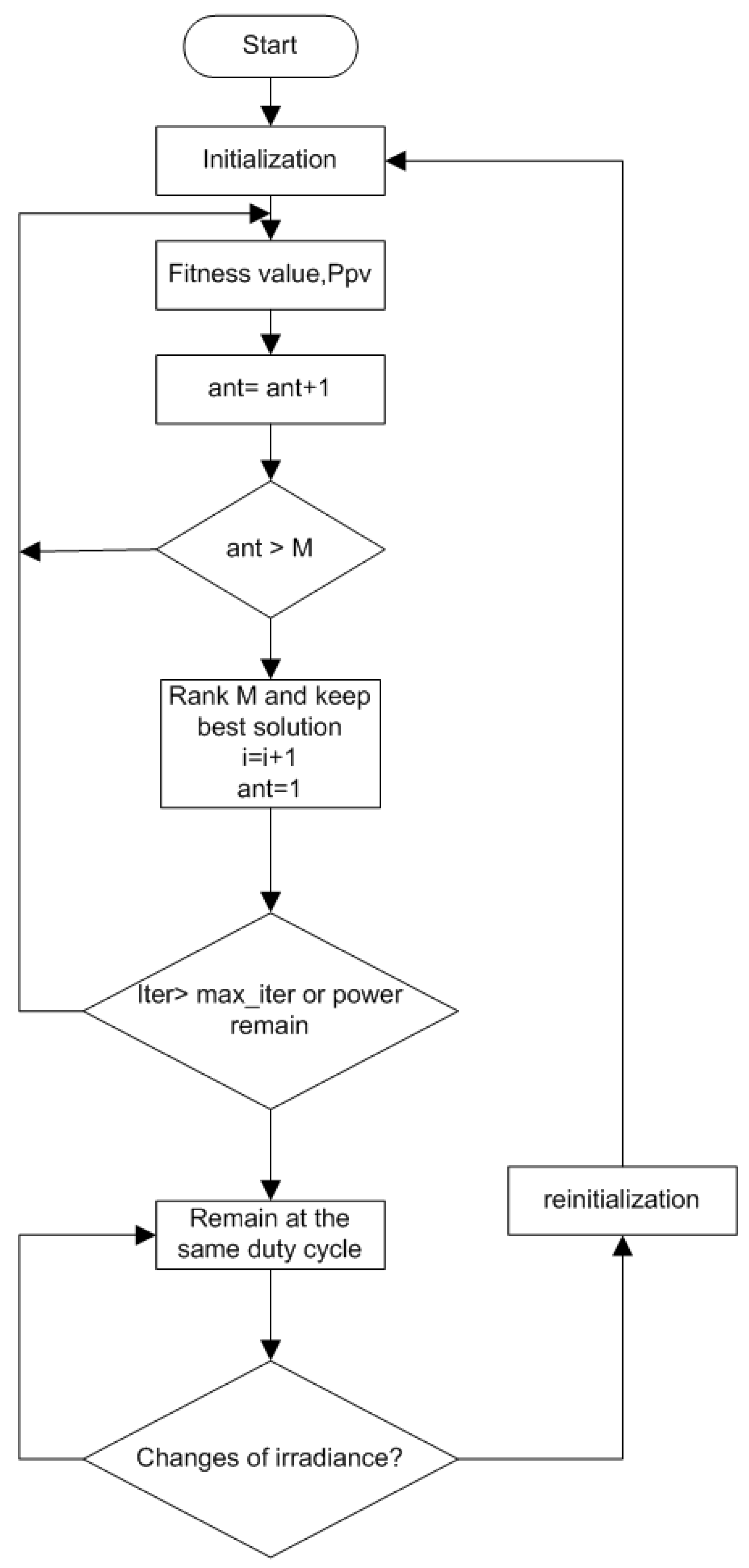
Ant colony optimization (ACO) is another swarm-based inspired algorithm. Normally, when searching for food, a single ant will leave a scent trail, which allows other ants to follow. The transition of knowledge shared between each other leads from poor to the best solution found [26,43]. Figure 3 shows a flowchart of the ACO in the MPPT application. ACO superiority performance is confirmed by few researchers over the conventional PSO in tracking the global optimum point [26,43]. It shows that its convergence is independent of its initial position and it has almost zero steady-state oscillations.
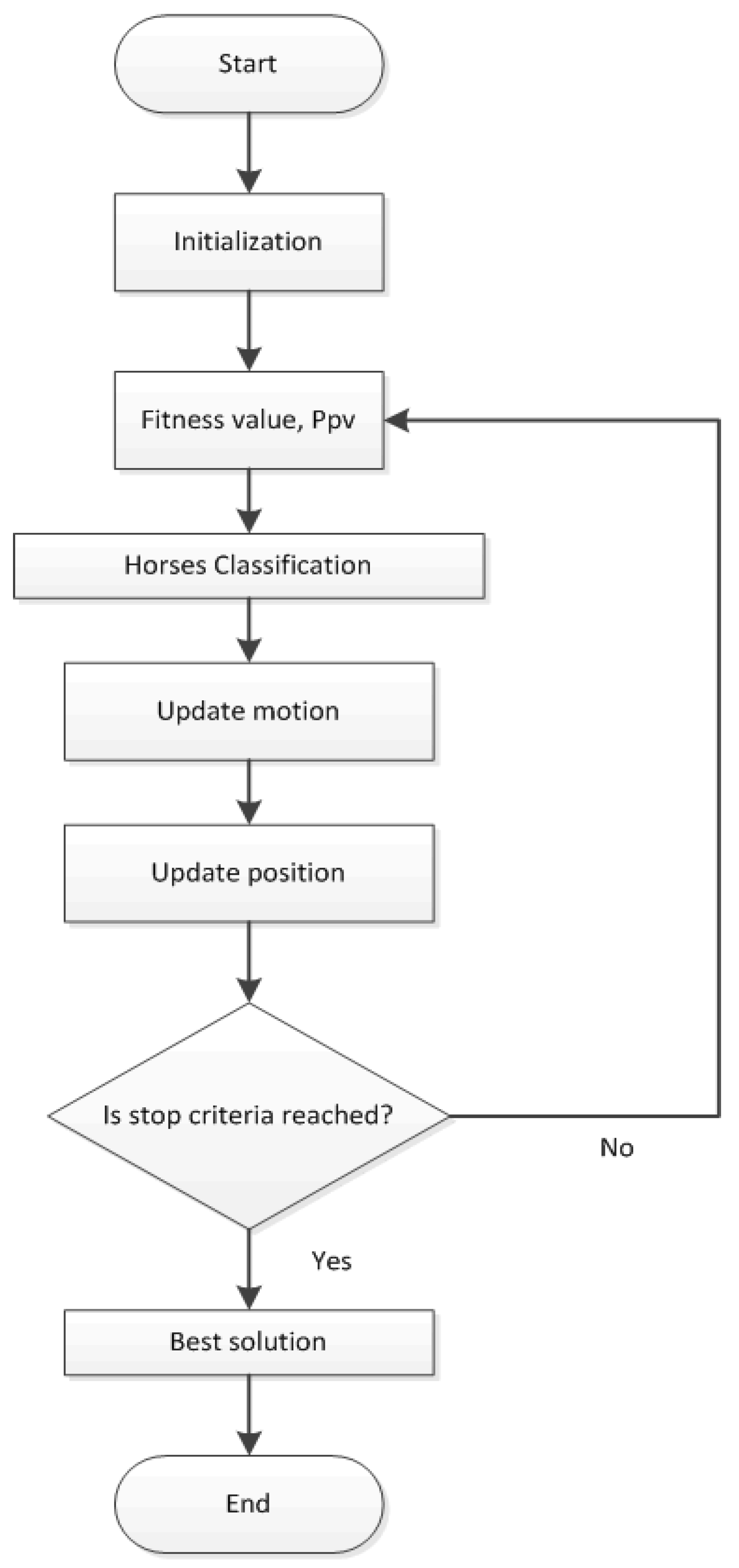
Another nature-inspired technique is horse herd optimization (HOA). This HOA technique is applied in the MPPT application by Sajid et. al. [13]. Figure 4 shows the flowchart of the HOA. In their findings, it shows that this HOA has superior performance under local and global tracking. Additionally, this algorithm only utilizes one single parameter in the search, resulting in zero steady-state oscillation and a fast tracking time.
Salp swarm algorithm (SSA) is inspired by a family of salps called Salpidae [16]. This family of salps have a transparent barrel-shaped body made of a tissue similar to that of a jellyfish. They move forward by pumping water similarly to jellyfishes. The exciting behavior of this family of salps is their ability to form a salp chain. The forming of a salps chain is still a mystery to researchers; however, it is believed that the formation of a chain is to coordinate changes in foraging [16]. It found that the parallel formation of salps chains is used in the exploration and exploitation of aid to better search for an optimum solution [16,29,30,31]. Figure 5 shows a flowchart of SSA in the MPPT application. Few researchers utilize this SSA in MPPT application, and based on their findings, this SSA shows a remarkable performance over other algorithms, with a high accuracy of tracking and low steady-state oscillations [16,31].
Table 1 shows a comparison of the existing algorithms used in the MPPT application based on the control scheme, type of the converter, pattern complexity, convergence speed, and tracking efficiency. Given the findings from 
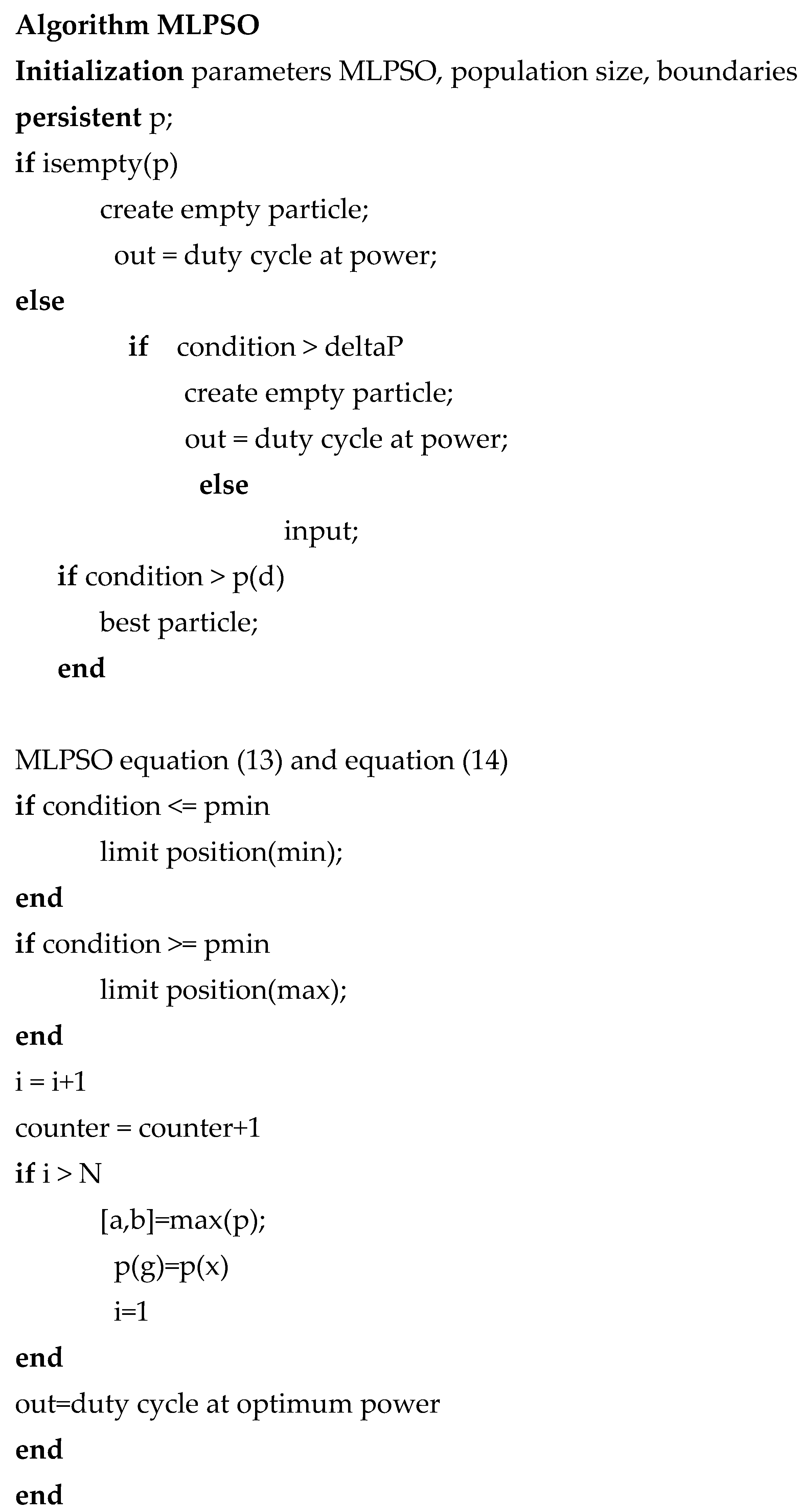
Table 1, it can be stated that Levy fight outperforms other nature-inspired algorithms in terms of tracking local and global optimum points with a high tracking speed and efficiency. Driven by the excellent performance of the Levy flight, shown in the table of comparison, the authors were inspired to propose a new modified Levy in the PV system. This paper discusses a modified Levy-PSO to improve the searching capability of the conventional PSO algorithm with a boost converter. The key concept here is to reduce the probability of getting trapped at the local point of the conventional PSO. Besides, the velocity is determined randomly based on the P-V characteristics. The proposed method provides few advantages, such as (a) the initial position of the particles are constant for each run and the solution depends on the randomness of the Levy flight search, (b) the merge and check process is added to increase the computational speed, (c) the boundary of the P-V curve is limited to Dmax for improving the search during rapid environmental change.
This paper is the extension from the previous paper as presented in [37]. In this paper, further evaluation on the effectiveness of the modified Levy flight-PSO with boost converter is studied more in-depth and is compared with the existing MPPT algorithms. Specifically, a detailed examination on the performance of the output boost converter, which has not been presented in [37], is now included in this paper.
The major contributions of this paper are listed as below:
  • A modified Levy-based particle swarm optimization with a boost converter is introduced with small swarm population.
  • Simulation and experiment verification of the proposed modified Levy-based particle swarm optimization with a boost converter.
  • Evaluate the performance of the proposed modified Levy-based particle swarm optimization with existing MPPT algorithm.
The rest of the paper is structured as follows. Section 2 discusses the analysis of the PV array under partial shading. Section 3 describes the conventional PSO, while 
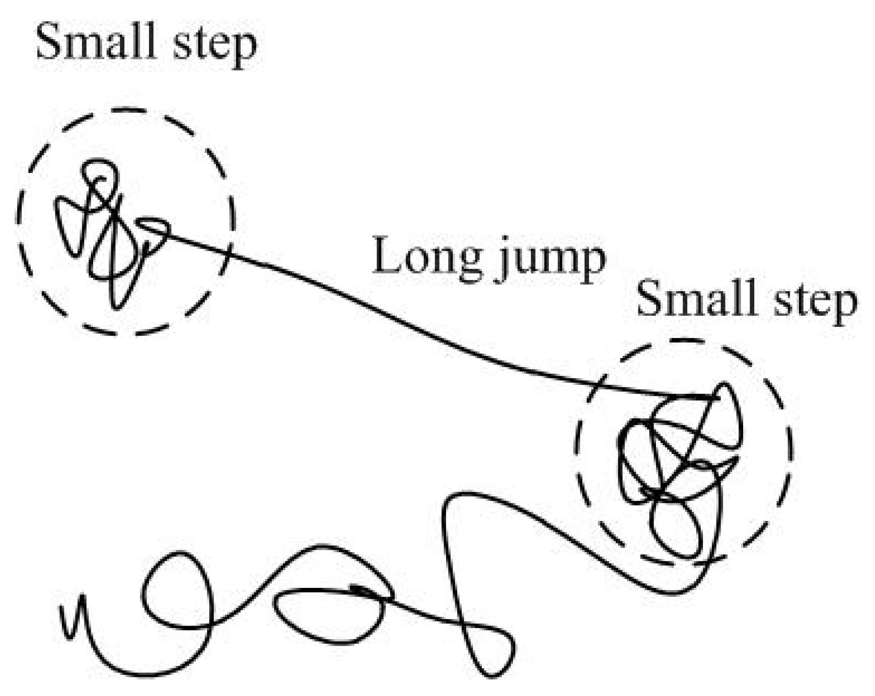
Section 4 describes the Levy flight search. Section 5 discusses the proposed modified Levy-PSO (MLPSO). In Section 6, the performance of the modified Levy-PSO is evaluated by a simulation, and Section 8 shows the simulation and experimental results. Finally, Section 9 provides the conclusion.

2. Analysis of PV System

2.1. Modeling of PV Cell under Partial Shading Condition

The analysis of a PV cell or module can be represented in either a single-diode or two-diode model [1,60]. The single-diode model comes with higher superiority in terms of simplicity and accuracy, which makes this model greatly preferable in most analysis [1,61].
The modeling of the PV cell is improved by adding reversed biased conditions in the circuit, as shown in Figure 6 [1,62]. The breakdown voltage is applied in the model [1,63]. The PV output current is given below [64]:
I = I ph I o ( e ( q ( V + R s I ) N s nKT ) 1 ) V + R s I R sh [ 1 + a ( 1 V + R s I V b ) β ]
where Iph is the current across the p–n junction (light generated current; this parameter depends upon the solar insolation), Io is the reverse saturation current of the cell, q is the electronics charge, V is the output voltage of the cell, Vb is breakdown voltage, a is 3, β is 2 × 10⁻³, Rs stands for the series resistance, n is the ideality factor, K is Boltzmann’s constant, T is the absolute operating temperature, Rsh is the shunt resistance (ideally infinity), Ns is the total number of cells connected in series, and Ish is the current flow through the shunt resistor. Given φ ( V ) is the leakage current.
Typically, the rated value for breakdown voltage is −15V [1,63]. Based on Equation (1), once partial shading occurs, the operating power is negative. The negative power indicates that the cell behaves as a load instead of a power source, therefore creating a phenomenon known as a hot spot [1,65]. This causes the targeted cell to function in a state of reverse-bias. High power is dissipated from the poor cell, which results in a higher temperature than normal, leading to destructive effects, such as solar cell degradation and glass cracking [66]. The most common solution is to add a bypass diode. The diode is connected in parallel with the cell to prevent the occurrence of a hot spot. Current is diverted to the alternative path, thus the reverse bias on PV strings is avoided [27,65,67]. However, the complexity in designing MPPT techniques is also increased.

2.2. Design of Boost Converter for Maximum Power Point Tracking

MPPT can only be applied by carefully designing the boost converter, especially under shading conditions [68]. Equation (2) shows the relationship of PV voltage and open-circuit voltage, Voc of the PV system under PSC [4].
V p v ( o p t ) , i ( n i + 1 ) n r v V o c
Given, Voc is the open-circuit terminal voltage of the PV array, n is the total number of peaks in the P-V curve, and rv is a constant (0.76 ≤ rv ≤ 0.82).
Equation (3) shows the relationship between the duty ratio of the boost converter and load resistance, Ro under PSC [69]:
R m ( max ) ( 1 d min ) 2 R l o a d ( o p t ) R m ( min ) ( 1 d max ) 2
where Rm(max) is the resistance at maximum power point at maximum irradiance, Rm(min) is the resistance at minimum power point at maximum irradiance, Rload(opt) is the optimum load resistance, and Dmax and Dmin are the minimum and maximum duty cycles, respectively. In the MPPT boost converter, the determination of optimum output resistance is necessary to ensure that the MPPT algorithm is not running at unlimited output resistance.
The value of the duty cycle of the boost converter depends on PV voltage and DC-link voltage. Equation (4) is used to determine the values of the duty cycle of the boost converter [4].
d i = 1 ( n i + 1 ) r v n x V o c V D C _ l i n k
The value of an inductor, L, is given in Equation (5) [69]:
L = R m Δ i L f ( 1 R m R l o a d )
where ∆iL is the inductor ripple current, Rm is the value of the resistance at the maximum power point, and f is the switching frequency.
The minimum input and output capacitance, Cin and Cout, are shown in Equations (6) and (7) [69]:
C i n = d 8 L γ V m f 2
where γVm is the voltage factor at the maximum power point.
C o = d ( 1 d ) 2 R m γ V o f

3. PSO in Tracking Global Peak

PSO is the iterative operation performed on a swarm of particles until an optimized solution is obtained [70,71]. Each particle in a swarm is guided by individual particles and the global best solution. These particles in a swarm are guided by two rules, which are the personal best particle, Pbest, and the global best particle, Pglobal. Particles are placed randomly in the search space. The next movement of a particle, Xi+1 is decided based on Equation (8):
x i k + 1 = x i k + v i k + 1
Given that velocity, v is the step size, which can be represented in Equation (9):
v i k + 1 = w v i k + c 1 r 1 { P b e s t i x i k } + c 2 r 2 { G b e s t x i k }
where w is inertia weight, c1 and c2 are the coefficients, r1 and r2 are randomly chosen numbers in between (0,1), Pbesti is i particle personal best, and Gbest is the global best in a swarm.
Amendments to the basic PSO formula are made to integrate it into the MPPT application. The modification is performed by defining the position by duty cycle and step size by velocity as shown in Equation (10):
d i k + 1 = d i k + v i k + 1
Equation (10) shows that any displacement of the duty cycle depends on the current duty cycle and velocity. By incorporating this equation into the PSO, the displacement of the duty cycle is varied based on the velocity [39].

4. Levy Flight Search in Tracking Global Peak

Levy flight was modeled by Paul Levy in 1937 from the behavior of animals looking for food [41]. The most important characteristic of Levy flight is the divergence in motion as shown in Figure 7 [36,42]. Levy flight distribution is presented by a power law as in Equation (11) [42]:
q = τ λ
where τ is the length of flight, and λ is the variance in between 1 < λ < 3.
The distribution of Levy flight is given by:
x k + 1 = x k + α L e v y ( λ )
where xk+1 is the next state, xk is the current state, α is step size and ⊗ is the product of entrywise multiplications. A modified Levy distribution is determined by:
q = α L e v y ( λ ) κ ( u | ν | 1 β 1 ) ( ν b e s t ν i ) + κ ( u | ν | 1 β 2 ) ( ν g l o b a l ν i )
where β is coefficient in between 0 ≤ β ≤ 2, K is the Levy multiplying coefficient, while u and υ are determined from normal distribution curves, i.e.,
u N ( 0 , σ u 2 )   and   ν N ( 0 , σ υ 2 )
Meanwhile, the variables σ u and are expressed in Equation (14) with the symbol Γ denoting the integral gamma function [36,72]:
σ u = ( Γ ( 1 + β ) x sin ( π x β / 2 ) Γ ( 1 + β 2 ) x β x 2 ( β 1 2 ) )   and   σ υ = 1

5. Proposed Modified Levy Particle Swarm Optimization

Initialization and Evaluation

The flowchart of the proposed MLPSO is shown in Figure 8. Firstly, all the particles are scattered at different locations in the search area using the following equation:
D = D i ,   I = 1 , 2 , 3 n
where D is the particle, and n is the total number of particles. Those particles are invoked successively at every iteration. The lower and upper boundaries are given by Dmin and Dmax, respectively. The particles D1, D2, D3 and D4 are initialized within the boundary of Dmin and Dmax. The particles are located on the right, middle, and left of the P-V curve. The initial power of the respective particle is stored as reference power. Consequently, D1 is initialized at Dmin, i.e.,
Pref(1) = PD1
Pref(2) is initialized at the left region of the P-V curve, i.e.,
Pref(2) = PD2
Pref(3) is initialized at the middle region of the P-V curve, i.e.,
Pref(3) = PD3
Finally, D4 is initialized at the rightmost region of P-V curve where at the maximum boundary of the P-V curve, i.e.,
Pref(4) = PD4
Using the PSO based in MLPSO, the particle motion is driven by the Levy random walk in the search. The step size of the invoked particle is guided by the best particle and global best as given in Equation (12). Once the best position, Pbest, is detected for particle Dn, the location is considered as LMPP. The respective particle, Dn, and power are stored as Pbest(Dn) and Dbest(Dn).
(1) Identification of new position
In MLPSO, random scanning of the P-V curve is performed. Figure 9 shows the mechanism movement of particles. Once the particles are invoked successively, the particle location is distributed into four regions again. During this stage, the respective Pbest and Dbest still hold the memory of the previous particle, where Pbest = Pbest(old). Then, the process of merge and check is executed to avoid the overlap scanning area along the P-V curve. The information about Pbest(old) and Pbest(new) is shared and checked as follows: Pbest(old) = Pbest(new) and Dbest(old) = Dbest(new). If there is another peak higher than Pbest(old), the new Pbest(new) is stored. A new LMPP corresponding to the MLPSO search is stored. This process is included to ensure that the entire search space between Dmin to Dmax is successfully evaluated.
(2) Final
After the MLPSO search has found GMPP at Pgbest, the search is reactivated. The step size of Levy is reduced to zero once all the particles reach their convergence. Furthermore, if there are any dynamic changes in the irradiance, the program is reinitialized as shown in Equation (21). The same process is executed again to locate a new GMPP.
| P p v P p v , o l d P p v , o l d | Δ P p v

6. Simulation

The effectiveness of the proposed MLPSO was verified by simulation. The simulation was constructed as shown in Figure 10. A standalone PV system was constructed which consisted of a PV array, a boost converter, and a resistive load. The details of the PV module used are shown in Table 2. The panel was used as a PV source. The voltage and current signals were sensed and fed to the MPPT controller where the variation of the duty cycle was depending on the optimum point of the P-V curve. The algorithm was implemented in the MATLAB function and the details of the algorithms are shown in Table 3. The voltage and current of the PV array were fed into the MATLAB function. The parameters of the boost converter are shown in Table 4. The sampling time for the MPPT was set at 0.1 s.
The characteristics of the PV module are shown in Figure 11. The details on the shading patterns are given in Table 5.
The non-uniform irradiance is created as shown in Figure 12. Non-uniform irradiance penetrates the PV array as given by Table 5. Three partial shading conditions are created, such as partial shading condition 1 (PSC 1), partial shading condition 2 (PSC 2), and partial shading condition 3 (PSC 3). Figure 13 shows the P-V and I-V curves for PSC 1, PSC 2, and PSC 3, respectively.

7. Experimental Setup

A prototype of a standalone PV system, as shown in Figure 10, was developed to verify the effectiveness of the proposed algorithms. PV Simulator, CHROMA 62100H-600S was used as the PV input source. The numerical data of the PV module, PMS50W was loaded into the CHROMA soft panel. The same patterns of irradiances were loaded in the PV simulator as in Table 6. The PV simulator was then connected to a boost converter. The boost converter consisted of an input capacitor, an inductor, a MOSFET, a diode, an output capacitor, and a DC electronic load. The PV voltage and current were sensed by a voltage sensor, LV25-P, and a current sensor, LA55-P, respectively. The sensed PV voltage and current were fed to a DSP TMS320F28335 controller. The output of the DSP TMS320F28335 was in the duty cycle. The proposed algorithm was implemented in the MATLAB function block and the details of the parameters of the proposed algorithms were as presented in Table 3. The output duty cycle was fed to a driver, HCPL 3120. The HCPL 3120 boosted the voltage up to +15 V. The PWM was then fed to the switching device, MOSFET. The variation of the PWM is depending on the optimum point of the irradiance of the system. Figure 14 shows the experimental setup for the proposed MPPT algorithm.

8. Results

8.1. Simulation Results

The performance of the proposed MLPSO with a boost converter was evaluated and tested. The proposed algorithms were compared with the conventional hill climbing (HC) and particle swarm optimization (PSO) methods. The duty cycle for each of the algorithms and the output performance for each algorithm are looked into in detail.
Figure 15 shows the simulation results for all MPPT algorithms tested under step-change in irradiance from 1000 W/m2 to 200 W/m2. The optimum power tracked by each of the algorithms is given, followed by the output voltage, current, and power of the converter. Based on the simulation results, the proposed MLPSO and LPSO showed an average output steady-state oscillation is 0.89%. This was mainly due to the Levy flight characteristic in which, once convergence is reached, the difference between a personal best and global best reaches zero, and the steady-state oscillation at the output converter will be zero as well. The HC method showed the worst performance with an average output power oscillation of 3.44%. This is mainly due to the characteristic of HC, which depends on the step size assigned in the search. Once the optimum point is reached, the point is still moving around the MPP vicinity point, causing a high output power oscillation at the converter. Meanwhile, the PSO had an average output power oscillation of 2.26%.
Table 7 shows the duty cycle for each of the MPPT algorithms tested under step-change of irradiance from 1000 W/m2 to 200 W/m2. Based on the simulation results, the optimum duty cycle under 1000 W/m2 was in the range of 0.61 to 0.62, and once abrupt changes of irradiance occurred at 200 W/m2, all the MPPT algorithms re-tracked the new optimum point by reregulating the duty cycle to look for a new optimum power with the optimum duty cycle in the range of 0.12 to 0.14.
Table 8 shows the performance of the output power converter for all MPPT algorithms tested under the step-change of irradiance from 1000 W/m2 to 200 W/m2. Based on the data given in Table 7, the proposed MLPSO showed overall system efficiency with an average efficiency of 99.10%. The LPSO showed an average efficiency of 99.34%. The PSO showed an average overall system efficiency of 97.73%. The worst overall system efficiency was given by the HC method with an average efficiency of 96.55%.
Figure 16 shows simulation results of the PV power, output voltage, current, and power for all MPPT algorithms tested under step-change of irradiance from PSC 1 to PSC 3. The proposed MLPSO and LPSO showed the best performance with the lowest steady-state oscillation with an average of 1.98%. The PSO contributed to an average steady-state output power oscillation of 6.27%. The HC method had the worst performance with an average steady-state oscillation of 33.00%.
Table 9 shows the duty cycle for all MPPT algorithms tested under step-change of irradiance from PSC 1 to PSC 3. Based on the data shown in Table 9, the proposed MLPSO and LPSO cleared its old memory of the optimum duty cycle at 0.73. Once there was any change in irradiance, the programs reregulated to look for a new GMPP at 0.50. In contrast, in the PSO and HC methods, the duty cycle remained constant regardless of irradiance change, with a constant duty cycle of 0.47 and 0.10, respectively, throughout the test.
Table 10 shows performance comparisons of the simulation results of the output converter for all MPPT algorithms tested under step-change of irradiance from PSC 1 to PSC 3. The proposed MLPSO showed an average converter efficiency of 98.01%. The LPSO showed an average converter efficiency of 98.22%. The PSO had an average converter efficiency of 93.76%. The worst performance was given by the HC method with an average converter efficiency of 66.99%.

8.2. Experimental Results

Figure 17 shows the experimental results for the PV current, PV voltage, PV power, and output voltage of the boost converter. The output voltage regulation for MLPSO was at 40.53 V. Once the step-change of irradiance occurred, the output voltage for the proposed MLPSO reregulated the output voltage to 19.37 V. The LPSO showed an output voltage of 40.66 V and reregulated the output to 20.01 V. Meanwhile, the output voltage regulation for the PSO algorithm was at 40.32 V and changed to 20.03 V, once the step-irradiance occurred under a low irradiance of 200 W/m2. The output voltage regulated up to 40.26 V for the HC method, and once step-change of irradiance was applied at the second interval, the output voltage was regulated to 19.81 V.
Table 11 shows the duty cycle of the boost converter tested under step-change of irradiance from 1000 W/m2 to 200 W/m2. All the algorithms can regulate the duty cycle under step-change of irradiance from 1000 W/m2 to 200 W/m2. Table 12 shows the performance comparison of the experimental results of the output boost converter for all the MPPT algorithms. The proposed MLPSO showed an average overall efficiency of 90.80%. The LPSO showed an average overall efficiency of 90.97%. The PSO had an average efficiency of 79.92%. The worst performance was given by the HC method with an average efficiency of 76.44%.
Figure 18 shows experimental results of the PV voltage, PV current, PV power, and output voltage of the converter tested under step-change of irradiance from PSC 1 to PSC 3. The proposed MLPSO showed that the output voltage was regulated to 23.53 V for PSC 1 and reregulated to 24.74 V when step-change of irradiance changed to PSC 3. The LPSO showed the output voltage of 40.66 V and reregulated to an output voltage of 20.16 V. The PSO showed the output voltage regulated to 22.55 V for PSC 1 and reregulated to 22.46 V when the change of irradiance occurred during the second interval. Meanwhile, the HC method showed the output voltage regulated at 21.34 V during PSC 1 and reregulated to 21.25 V after the step-change of irradiance at PSC 3.
Table 13 shows the performance comparison of the experimental results of the duty cycle between the proposed MLPSO method and the existing HC and PSO methods under step-change of irradiance from PSC 1 to PSC 3. The proposed MLPSO and LPSO regulated the duty cycle at 0.67 during PSC 1 and reregulated to a duty cycle at 0.45 once the step-change of irradiance at PSC 3 occurred. In contrast, the PSO regulated to duty cycle of 0.38 during PSC 1, indicating that the algorithm was stuck at the LMPP, and thus, still executing the same duty cycle during PSC 3. This means that the PSO did not clear its old memory but was still holding to the same memory of the previous duty cycle at 0.38. The HC method, in particular, was unable to regulate its duty cycle under partial shading conditions as the duty cycle was at 0.05 for PSC 1 and 0.07 for PSC 3.
Table 14 shows the performance comparison of the experimental results of the output boost converter for the HC, PSO, and MLPSO algorithms tested under step-change of irradiance from PSC 1 to PSC 3. The proposed MLPSO showed an average efficiency of 85.29%. LPSO showed an average overall system efficiency of 85.57%. The second-best performance was given by the PSO with an average efficiency of 73.05%. The worst performance was contributed by the HC method with an average efficiency of 46.73%.
The efficiency of the MPPT tracking is the ratio of the tracked output PV power by MPPT algorithm to the desired PV power. The proposed MLPSO and LPSO showed an average MPPT tracking efficiency of 99.50%. The efficiency of the PSO was at an average of 92.57%. The MPPT tracking efficiency of the HC method was at an average of 64.57%.
The HC method showed the poorest range of MPPT tracking efficiency compared to other methods, due to high steady-state oscillation and its failure to track optimum power under partial shading conditions. The HC method uses a curve identification method in its search, which depends on the incremental and decremental step size in the search area. The fixed step size used in the search causes the point to still move around the vicinity point even when the optimum point is reached. This causes a continuous steady-state oscillation, which significantly lowers the tracking efficiency. The inability to work under a partial shading condition is due to its inability to retain memory. The comparison is only conducted by comparing the obtained instant power with the previous power and the increment and decrement of the step size are decided based on that instant power.
In contrast, the PSO, LPSO, and MLPSO methods utilized the search-based method of the search. This method has a high capability to work under complex situations, such as under partial shading conditions. In these methods, once the optimum point is reached, it remains unchanged. Since there is no longer any difference between the best particle and the global best particle, zero steady-state oscillation occurs, resulting in higher efficiency compared with the curve identification method. Furthermore, Levy flight, used in the search, enhances the global search capability by covering the overlooked point of the PSO method. The PSO method has intermittent tracking under partial shading due to random initialization used in the search. The number of particles limits the search capability of the PSO method. Here, only four particles are used in the search area. In the proposed modified Levy, the same numbers of particles are used in the search area. However, due to the nature of Levy flight, especially under partial shading conditions, the search of the global point is successfully achieved. In the proposed modified Levy particle swarm, once the modified Levy flight is activated, the points overlooked by the conventional PSO are once again covered by modified Levy flight.
Table 15 shows a performance comparison of the proposed MPPT algorithm with other AI methods. The proposed MPPT algorithm has improved the efficiency by approximately 0.41% to 21.72%, compared to the power-increment, MSSA and GSO, methods. However, the proposed method shows a slightly slow response time compared to other MPPT methods. This is mainly due to the sample time used in both the simulation and experiment. Sample time is the time taken for the algorithm to sample its input. In MPPT algorithms, this sample time plays a significant role in determining the total time to reach the steady-state. The smaller the sample time set to the system, the faster the algorithm reaches the steady-state. However, if a bigger number is chosen, a longer time is needed to reach the steady-state. In this research study, the sample time was chosen at 0.10 due to the best match between software and hardware. Thus, the obtained results are the best compromise for this experiment set-up. However, if a smaller sample time is chosen, the proposed MPPT algorithm should have a faster time as modified Levy flight is utilized in the search. In addition, the modification was performed at the local region in which the randomness was enhanced by covering the local region, while in the previous research proposed in [1], the LPSO randomness only covered the second region, which was at the global region. A random step size, obtained for each iteration, would expedite the local and global search in the system. This would improve the tracking speed of the system.

9. Conclusions

This paper presented a MLPSO algorithm for local and global maximum power point tracking with a boost converter. The proposed MLPSO only used four duty cycles in its search. In the MPPT application, the tradeoff between the population size and the convergence speed was the major concern. A small population size results in faster convergence times, whereas a large population size has higher success rates but with slower convergence times. Additionally, a large population size also has a high possibility of being unable to respond quickly to the rapid changes of the environment. Thus, due to these constraints, in this paper, Levy flight was employed with some modifications performed on the parameters, contributing to great findings on the mobility of the particles. In the proposed technique, the search was utilized by Levy flight based on PSO. The diversity of the PSO was expended by adding a β parameter to the search. The efficiency of the proposed MLPSO was also critically examined under step-change of irradiance by both a simulation and experiment. The proposed MLPSO was also compared with the existing methods, HC and PSO. The results demonstrated that the proposed method comes with an excellent performance in tracking speed of approximately 1.5 to 3.0 s, average output steady-state oscillation of 0.89%, and an overall system efficiency with an average efficiency of 99.10%. Furthermore, if compared to other MPPT methods, the proposed MPPT algorithm has almost as high an efficiency as any other AI methods. This is due to the search-based technique utilized in the system. Search-based techniques have high efficiency, low steady-state oscillation, and a good capability to work under complex conditions. Moreover, the sample time can also be set to a smaller value as it allows a faster convergence time as observed in other AI MPPT techniques.

Author Contributions

C.C. developed the simulation model, algorithm, conducted the tests, analyzed all the important findings, and wrote the manuscript; D.I. verified the simulation study, and experimental and written manuscript; M.A.A.M.Z. verified the methodology, and revised and finalized the drafted manuscript. B.I. revised and finalized the drafted manuscript. T.A. revised and finalized the final manuscript. A.R.H.A. revised and finalized the final manuscript. All authors have read and agreed to the published version of the manuscript.

Funding

This research received no external funding.

Institutional Review Board Statement

Not applicable.

Informed Consent Statement

Not applicable.

Data Availability Statement

Not applicable.

Acknowledgments

This research work is supported by Fundamental Research Grant Scheme FRGS/1/2020/TK0/UKM/02/11 by the Ministry of Higher Education Malaysia.

Conflicts of Interest

The authors declare no conflict of interest.

References

  1. Da Luz, C.M.A.; Vicente, E.M.; Tofoli, F.L. Experimental evaluation of global maximum power point techniques under partial shading conditions. Sol. Energy 2020, 196, 49–73. [Google Scholar] [CrossRef]
  2. Saravanan, S.; Babu, N.R. Maximum power point tracking algorithms for photovoltaic system–A review. Renew. Sustain. Energy Rev. 2016, 57, 192–204. [Google Scholar] [CrossRef]
  3. Ahmed, J.; Salam, Z. An improved perturb and observe (P&O) maximum power point tracking (MPPT) algorithm for higher efficiency. Appl. Energy 2015, 150, 97–108. [Google Scholar]
  4. Eltamaly, A.M.; Al-Saud, M.; Abokhalil, A.G.; Farh, H.M. Simulation and experimental validation of fast adaptive particle swarm optimization strategy for photovoltaic global peak tracker under dynamic partial shading. Renew. Sustain. Energy Rev. 2020, 124, 109719. [Google Scholar] [CrossRef]
  5. Eltamaly, A.M.; Farh, H.M. Dynamic global maximum power point tracking of the PV systems under variant partial shading using hybrid GWO-FLC. Sol. Energy 2019, 177, 306–316. [Google Scholar] [CrossRef]
  6. Saidi, K.; Maamoun, M.; Bounekhla, M.H. A new high performance variable step size perturb-and-observe MPPT algorithm for photovoltaic system. Int. J. Power Electron. Drive Syst. 2019, 10, 1662. [Google Scholar] [CrossRef]
  7. Killi, M.; Samanta, S. Modified perturb and observe MPPT algorithm for drift avoidance in photovoltaic systems. IEEE Trans. Ind. Electron. 2015, 62, 5549–5559. [Google Scholar] [CrossRef]
  8. Elgendy, M.; Zahawi, B.; Atkinson, D. Evaluation of perturb and observe MPPT algorithm implementation techniques. 2012, 2012, pp 1–6. In Proceedings of the IET International Conference on Power Electronics, Machines and Drives 2012 (PEMD 2012), Bristol, UK, 27–29 March 2012; pp. 1–6. [Google Scholar]
  9. Jiang, Y.; Qahouq, J.A.A.; Haskew, T.A. Adaptive step size with adaptive-perturbation-frequency digital MPPT controller for a single-sensor photovoltaic solar system. IEEE Trans. Power Electron. 2012, 28, 3195–3205. [Google Scholar] [CrossRef]
  10. Sarwar, S.; Javed, M.Y.; Jaffery, M.H.; Ashraf, M.S.; Naveed, M.T.; Hafeez, M.A. Modular Level Power Electronics (MLPE) Based Distributed PV System for Partial Shaded Conditions. Energies 2022, 15, 4797. [Google Scholar] [CrossRef]
  11. Ramli, M.Z.; Salam, Z. Performance evaluation of dc power optimizer (DCPO) for photovoltaic (PV) system during partial shading. Renew. Energy 2019, 139, 1336–1354. [Google Scholar] [CrossRef]
  12. Ahmed, J.; Salam, Z. An enhanced adaptive P&O MPPT for fast and efficient tracking under varying environmental conditions. IEEE Trans. Sustain. Energy 2018, 9, 1487–1496. [Google Scholar]
  13. Sarwar, S.; Hafeez, M.A.; Javed, M.Y.; Asghar, A.B.; Ejsmont, K. A Horse Herd Optimization Algorithm (HOA)-Based MPPT Technique under Partial and Complex Partial Shading Conditions. Energies 2022, 15, 1880. [Google Scholar] [CrossRef]
  14. Alik, R.; Jusoh, A. Modified Perturb and Observe (P&O) with checking algorithm under various solar irradiation. Sol. Energy 2017, 148, 128–139. [Google Scholar]
  15. Alshareef, M.; Lin, Z.; Ma, M.; Cao, W. Accelerated particle swarm optimization for photovoltaic maximum power point tracking under partial shading conditions. Energies 2019, 12, 623. [Google Scholar] [CrossRef] [Green Version]
  16. Yang, B.; Zhong, L.; Zhang, X.; Shu, H.; Yu, T.; Li, H.; Jiang, L.; Sun, L. Novel bio-inspired memetic salp swarm algorithm and application to MPPT for PV systems considering partial shading condition. J. Clean. Prod. 2019, 215, 1203–1222. [Google Scholar] [CrossRef]
  17. Avila, L.; De Paula, M.; Trimboli, M.; Carlucho, I. Deep reinforcement learning approach for MPPT control of partially shaded PV systems in Smart Grids. Appl. Soft Comput. 2020, 97, 106711. [Google Scholar] [CrossRef]
  18. Manickam, C.; Raman, G.; Raman, G.; Ganesan, S.; Nagamani, C. A hybrid algorithm for tracking of global MPP based on perturb and observe and particle swarm optimization with reduced power oscillation in string inverters. IEEE Trans. Ind. Electron. 2016, 63, 6097–6106. [Google Scholar] [CrossRef]
  19. Ramli, M.A.; Twaha, S.; Ishaque, K.; Al-Turki, Y.A. A review on maximum power point tracking for photovoltaic systems with and without shading conditions. Renew. Sustain. Energy Rev. 2017, 67, 144–159. [Google Scholar] [CrossRef]
  20. Baba, A.O.; Liu, G.; Chen, X. Classification and Evaluation Review of Maximum Power Point Tracking Methods. Sustain. Futures 2020, 2, 100020. [Google Scholar] [CrossRef]
  21. Pilakkat, D.; Kanthalakshmi, S. An improved P&O algorithm integrated with artificial bee colony for photovoltaic systems under partial shading conditions. Sol. Energy 2019, 178, 37–47. [Google Scholar]
  22. Zhao, Z.; Cheng, R.; Yan, B.; Zhang, J.; Zhang, Z.; Zhang, M.; Lai, L.L. A dynamic particles MPPT method for photovoltaic systems under partial shading conditions. Energy Convers. Manag. 2020, 220, 113070. [Google Scholar] [CrossRef]
  23. Rajendran, S.; Srinivasan, H. Simplified accelerated particle swarm optimisation algorithm for efficient maximum power point tracking in partially shaded photovoltaic systems. IET Renew. Power Gener. 2016, 10, 1340–1347. [Google Scholar] [CrossRef]
  24. Tajuddin, M.F.N.; Ayob, S.M.; Salam, Z. In Tracking of maximum power point in partial shading condition using differential evolution (DE). In Proceedings of the 2012 IEEE International Conference on Power and Energy (PECon), IEEE, Kota Kinabalu, Sabah, 2–5 December 2012; pp. 384–389. [Google Scholar]
  25. Seyedmahmoudian, M.; Rahmani, R.; Mekhilef, S.; Oo, A.M.T.; Stojcevski, A.; Soon, T.K.; Ghandhari, A.S. Simulation and hardware implementation of new maximum power point tracking technique for partially shaded PV system using hybrid DEPSO method. IEEE Trans. Sustain. Energy 2015, 6, 850–862. [Google Scholar] [CrossRef]
  26. Phanden, R.K.; Sharma, L.; Chhabra, J.; Demir, H.İ. A novel modified ant colony optimization based maximum power point tracking controller for photovoltaic systems. Mater. Today: Proc. 2021, 38, 89–93. [Google Scholar] [CrossRef]
  27. Soufyane Benyoucef, A.; Chouder, A.; Kara, K.; Silvestre, S. Artificial bee colony based algorithm for maximum power point tracking (MPPT) for PV systems operating under partial shaded conditions. Appl. Soft Comput. 2015, 32, 38–48. [Google Scholar] [CrossRef] [Green Version]
  28. Eltamaly, A.M. A novel musical chairs algorithm applied for MPPT of PV systems. Renew. Sustain. Energy Rev. 2021, 146, 111135. [Google Scholar] [CrossRef]
  29. Premkumar, M.; Ibrahim, A.M.; Kumar, R.M.; Sowmya, R. Analysis and Simulation of Bio-Inspired Intelligent Salp Swarm MPPT Method for the PV Systems under Partial Shaded Conditions. Int. J. Comput. Digit. Syst. 2019, 8, 490–496. [Google Scholar]
  30. Premkumar, M.; Kumar, C.; Sowmya, R.; Pradeep, J. A novel salp swarm assisted hybrid maximum power point tracking algorithm for the solar photovoltaic power generation systems. Automatika 2020, 62, 1–20. [Google Scholar] [CrossRef]
  31. Jamaludin, M.N.I.; Tajuddin, M.F.N.; Ahmed, J.; Azmi, A.; Azmi, S.A.; Ghazali, N.H.; Babu, T.S.; Alhelou, H.H. An Effective Salp Swarm Based MPPT for Photovoltaic Systems Under Dynamic and Partial Shading Conditions. IEEE Access 2021, 9, 34570–34589. [Google Scholar] [CrossRef]
  32. Mansoor, M.; Mirza, A.F.; Ling, Q.; Javed, M.Y. Novel Grass Hopper optimization based MPPT of PV systems for complex partial shading conditions. Sol. Energy 2020, 198, 499–518. [Google Scholar] [CrossRef]
  33. Zainuri, M.A.A.M.; Radzi, M.A.M.; Soh, A.C.; Abd Rahim, N. Development of adaptive perturb and observe-fuzzy control maximum power point tracking for photovoltaic boost dc–dc converter. IET Renew. Power Gener. 2013, 8, 183–194. [Google Scholar] [CrossRef]
  34. Hashemzadeh, S.M. A new model-based technique for fast and accurate tracking of global maximum power point in photovoltaic arrays under partial shading conditions. Renew. Energy 2019, 139, 1061–1076. [Google Scholar] [CrossRef]
  35. Haklı, H.; Uğuz, H. A novel particle swarm optimization algorithm with Levy flight. Appl. Soft Comput. 2014, 23, 333–345. [Google Scholar] [CrossRef]
  36. Charin, C.; Ishak, D.; Mohd Zainuri, M.A.A.; Ismail, B. Modified Levy Flight Optimization for a Maximum Power Point Tracking Algorithm under Partial Shading. Appl. Sci. 2021, 11, 992. [Google Scholar] [CrossRef]
  37. Charin, C.; Ishak, D.; Mohd Zainuri, M.A.A.; Ismail, B.; Mohd Jamil, M.K. A hybrid of bio-inspired algorithm based on Levy flight and particle swarm optimizations for photovoltaic system under partial shading conditions. Sol. Energy 2021, 217, 1–14. [Google Scholar]
  38. Ishaque, K.; Salam, Z. A deterministic particle swarm optimization maximum power point tracker for photovoltaic system under partial shading condition. IEEE Trans. Ind. Electron. 2012, 60, 3195–3206. [Google Scholar] [CrossRef]
  39. Ishaque, K.; Salam, Z.; Amjad, M.; Mekhilef, S. An improved particle swarm optimization (PSO)–based MPPT for PV with reduced steady-state oscillation. IEEE Trans. Power Electron. 2012, 27, 3627–3638. [Google Scholar] [CrossRef]
  40. Bendib, B.; Belmili, H.; Krim, F. A survey of the most used MPPT methods: Conventional and advanced algorithms applied for photovoltaic systems. Renew. Sustain. Energy Rev. 2015, 45, 637–648. [Google Scholar]
  41. Islam, H.; Mekhilef, S.; Shah, N.B.M.; Soon, T.K.; Seyedmahmousian, M.; Horan, B.; Stojcevski, A. Performance evaluation of maximum power point tracking approaches and photovoltaic systems. Energies 2018, 11, 365. [Google Scholar]
  42. Ahmed, J.; Salam, Z. A Maximum Power Point Tracking (MPPT) for PV system using Cuckoo Search with partial shading capability. Appl. Energy 2014, 119, 118–130. [Google Scholar] [CrossRef]
  43. Priyadarshi, N.; Ramachandaramurthy, V.; Padmanaban, S.; Azam, F. An Ant Colony Optimized MPPT for Standalone Hybrid PV-Wind Power System with Single Cuk Converter. Energies 2019, 12, 167. [Google Scholar] [CrossRef] [Green Version]
  44. Chandrasekaran, K.; Sankar, S.; Banumalar, K. Partial shading detection for PV arrays in a maximum power tracking system using the sine-cosine algorithm. Energy Sustain. Dev. 2020, 55, 105–121. [Google Scholar] [CrossRef]
  45. Karmouni, H.; Chouiekh, M.; Motahhir, S.; Qjidaa, H.; Ouazzani Jamil, M.; Sayyouri, M. A fast and accurate sine-cosine MPPT algorithm under partial shading with implementation using arduino board. Clean. Eng. Technol. 2022, 9, 100535. [Google Scholar] [CrossRef]
  46. Aquib, M.; Jain, S. A Global Maximum Power Point Tracking Technique Based on Current Source Region Detection of I-V Curve. In Proceedings of the 2018 IEEMA Engineer Infinite Conference (eTechNxT), New Delhi, India, 13–14 March 2018. [Google Scholar]
  47. Li, X.; Wen, H.; Chu, G.; Hu, Y.; Jiang, L. A novel power-increment based GMPPT algorithm for PV arrays under partial shading conditions. Sol. Energy 2018, 169, 353–361. [Google Scholar] [CrossRef]
  48. Furtado, A.M.S.; Bradaschia, F.; Cavalcanti, M.C.; Limongi, L.R. A Reduced Voltage Range Global Maximum Power Point Tracking Algorithm for Photovoltaic Systems Under Partial Shading Conditions. IEEE Trans. Ind. Electron. 2018, 65, 3252–3262. [Google Scholar] [CrossRef]
  49. Jately, V.; Azzopardi, B.; Joshi, J.; Venkateswaran, B.; Sharma, A.; Arora, S. Experimental Analysis of hill-climbing MPPT algorithms under low irradiance levels. Renew. Sustain. Energy Rev. 2021, 150, 111467. [Google Scholar] [CrossRef]
  50. Kalogerakis, C.; Koutroulis, E.; Lagoudakis, M.G. Global MPPT Based on Machine-Learning for PV Arrays Operating under Partial Shading Conditions. Appl. Sci. 2020, 10, 700. [Google Scholar] [CrossRef] [Green Version]
  51. Li, X.; Wen, H.; Hu, Y.; Jiang, L. A novel beta parameter based fuzzy-logic controller for photovoltaic MPPT application. Renew. Energy 2019, 130, 416–427. [Google Scholar] [CrossRef]
  52. Sundararaj, V.; Anoop, V.; Dixit, P.; Arjaria, A.; Chourasia, U.; Bhambri, P.M.R.R.; Sundararaj, R. CCGPA-MPPT: Cauchy preferential crossover-based global pollination algorithm for MPPT in photovoltaic system. Prog. Photovolt. Res. Appl. 2020, 28, 1128–1145. [Google Scholar] [CrossRef]
  53. Ram, J.P.; Pillai, D.S.; Ghias, A.M.Y.M.; Rajasekar, N. Performance enhancement of solar PV systems applying P&O assisted Flower Pollination Algorithm (FPA). Sol. Energy 2020, 199, 214–229. [Google Scholar]
  54. Hamdi, H.; Ben Regaya, C.; Zaafouri, A. Real-time study of a photovoltaic system with boost converter using the PSO-RBF neural network algorithms in a MyRio controller. Sol. Energy 2019, 183, 1–16. [Google Scholar] [CrossRef]
  55. Mo, S.; Ye, Q.; Jiang, K.; Mo, X.; Shen, G. An improved MPPT method for photovoltaic systems based on mayfly optimization algorithm. Energy Rep. 2022, 8, 141–150. [Google Scholar] [CrossRef]
  56. Chen, L.; Li, Z.; Zhang, Y.; Zhang, Y. An improved quantum particle swarm photovoltaic multi-peak mPPT method combined with Lévy flight. Energy Sci. Eng. 2020, 8, 3980–3994. [Google Scholar] [CrossRef]
  57. Mansoor, M.; Mirza, A.F.; Ling, Q. Harris hawk optimization-based MPPT control for PV systems under partial shading conditions. J. Clean. Prod. 2020, 274, 122857. [Google Scholar] [CrossRef]
  58. Fathy, A.; Atitallah, A.B.; Yousri, D.; Rezk, H.; Al-Dhaifallah, M. A new implementation of the MPPT based raspberry Pi embedded board for partially shaded photovoltaic system. Energy Rep. 2022, 8, 5603–5619. [Google Scholar] [CrossRef]
  59. Gupta, S.; Saurabh, K. Modified Artificial Killer Whale Optimization Algorithm for Maximum Power Point Tracking under Partial Shading Condition. In Proceedings of the 2017 International Conference on Recent Trends in Electrical, Electronics and Computing Technologies (ICRTEECT), Warangal, India, 30–31 July 2017; pp. 87–92. [Google Scholar]
  60. Mohanty, S.; Subudhi, B.; Ray, P.K. A grey wolf-assisted perturb & observe MPPT algorithm for a PV system. IEEE Trans. Energy Convers. 2016, 32, 340–347. [Google Scholar]
  61. Lo Brano, V.; Orioli, A.; Ciulla, G.; Di Gangi, A. An improved five-parameter model for photovoltaic modules. Sol. Energy Mater. Sol. Cells 2010, 94, 1358–1370. [Google Scholar] [CrossRef]
  62. Spirito, P.; Albergamo, V. In Reverse Bias Power Dissipation of Shadowed or Faulty Cells in Different Array Configurations. In Proceedings of the Fourth EC Photovoltaic Solar Energy Conference, Stresa, Italy, 10–14 May 1982; Springer: Berlin/Heidelberg, Germany, 1982; pp. 296–300. [Google Scholar]
  63. Silvestre, S.; Boronat, A.; Chouder, A. Study of bypass diodes configuration on PV modules. Appl. Energy 2009, 86, 1632–1640. [Google Scholar] [CrossRef]
  64. Bishop, J. Computer simulation of the effects of electrical mismatches in photovoltaic cell interconnection circuits. Sol. Cells 1988, 25, 73–89. [Google Scholar] [CrossRef]
  65. Ghasemi, M.A.; Foroushani, H.M.; Parniani, M. Partial shading detection and smooth maximum power point tracking of PV arrays under PSC. IEEE Trans. Power Electron. 2015, 31, 6281–6292. [Google Scholar] [CrossRef]
  66. Veerapen, S.; Wen, H.; Li, X.; Du, Y.; Yang, Y.; Wang, Y.; Xiao, W. A novel global maximum power point tracking algorithm for photovoltaic system with variable perturbation frequency and zero oscillation. Sol. Energy 2019, 181, 345–356. [Google Scholar] [CrossRef]
  67. Hajighorbani, S.; Radzi, M.A.M.; Kadir, M.Z.A.A.; Shafie, S. Dual search maximum power point (dsmpp) algorithm based on mathematical analysis under shaded conditions. Energies 2015, 8, 12116–12146. [Google Scholar] [CrossRef] [Green Version]
  68. Hajighorbani, S.; Mohd Radzi, M.A.; Ab Kadir, M.Z.A.; Shafie, S.; Mohd Zainuri, M.A.A. Implementing a novel hybrid maximum power point tracking technique in DSP via Simulink/MATLAB under partially shaded conditions. Energies 2016, 9, 85. [Google Scholar] [CrossRef] [Green Version]
  69. Ayop, R.; Tan, C.W. Design of boost converter based on maximum power point resistance for photovoltaic applications. Sol. Energy 2018, 160, 322–335. [Google Scholar] [CrossRef]
  70. Koad, R.B.; Zobaa, A.F. Comparison between the conventional methods and PSO based MPPT algorithm for photovoltaic systems. World Acad. Sci. Eng. Technol. 2014, 8. [Google Scholar]
  71. Abdullah, M.A.; Al-Hadhrami, T.; Tan, C.W.; Yatim, A.H. Towards green energy for smart cities: Particle swarm optimization based MPPT approach. IEEE Access 2018, 6, 58427–58438. [Google Scholar] [CrossRef]
  72. Heidari, A.A.; Pahlavani, P. An efficient modified grey wolf optimizer with Lévy flight for optimization tasks. Appl. Soft Comput. 2017, 60, 115–134. [Google Scholar] [CrossRef]
Figure 1. Conventional PSO in MPPT application [15].
Energies 15 07370 g001
Figure 2. Cuckoo Search Algorithm.
Energies 15 07370 g002
Figure 3. Ant colony optimization (ACO) [26,43].
Energies 15 07370 g003
Figure 4. Horse Herd Optimization (HOA) [13].
Energies 15 07370 g004
Figure 5. Salp swarm algorithm (SSA) [16].
Energies 15 07370 g005
Figure 6. Photovoltaic cell with breakdown voltage, φ(V).
Energies 15 07370 g006
Figure 7. Levy flight distribution.
Energies 15 07370 g007
Figure 8. Pseudo code for MLPSO.
Energies 15 07370 g008
Figure 9. Mechanism of the Levy-PSO (a) re-initialization, (b) movement of the particle D1, (c) movement of the particle D2, (d) movement of particle D3, (e) movement of particle D4, and (f) particles D1, D2, D3, and D4 converge at global point.
Energies 15 07370 g009
Figure 10. Schematic of a standalone PV system.
Energies 15 07370 g010
Figure 11. (a) I-V and (b) P-V curves of PMS50W at high (1000 W/m2), medium (600 W/m2), and low (200 W/m2) irradiances.
Energies 15 07370 g011
Figure 12. Non-uniform irradiance penetrated to PV array.
Energies 15 07370 g012
Figure 13. (a) I-V curves and (b) P-V curves for PSC 1, PSC 2, and PSC 3.
Energies 15 07370 g013
Figure 14. Experimental apparatus and setup.
Energies 15 07370 g014
Figure 15. Simulation results of the PV power, output voltage, output current, and output power of the boost converter under step-change of irradiance from 1000 W/m2 to 200 W/m2 for (a) HC, (b) PSO, (c) LPSO, and (d) MLPSO.
Energies 15 07370 g015aEnergies 15 07370 g015b
Figure 16. Simulation results of the PV power, output voltage, output current, and output power of the boost converter under step-change of irradiance from PSC 1 to PSC 3 for (a) HC, (b) PSO, (c) LPSO, and (d) MLPSO.
Energies 15 07370 g016aEnergies 15 07370 g016b
Figure 17. Experimental results of the PV current, PV voltage, PV power, and output voltage of the boost converter under step-change from 1000 W/m2 to 200 W/m2 for (a) HC, (b) PSO, (c) LPSO, and (d) MLPSO.
Energies 15 07370 g017
Figure 18. Experimental results of the PV current, PV voltage, PV power and output voltage of the boost converter under step-change from PSC 1 to PSC 3 for (a) HC (b) PSO (c) LPSO and (d) MLPSO.
Energies 15 07370 g018
Table 1. Comparative performance of MPPT algorithms by other researchers.
Tracking Technique with Measurement and Comparison/Mathematical Calculation
AuthorMPPTConverterCaseResponse Time (s)Efficiency (%)
PSC Peak (No.)Power (W)
Sine-cosine
Chandrasekaran [44]SCA-ISCABoost21.2 k1.6095.06
Hicham [45]SCAMCUK44000.6299.93%
Current
Aquib, Mohd [46]CSRBoost259.90<3.00>99.90
Xingshuo Li [47]Power-incrementBuck-boost360.008.0077.78
Furtado, Artur M.S. [48]MPT-High complexity>1500<0.30high
Hill climbing
Jately [49]Hill-climbingBoostUniform151.4>90%
Tracking technique with intelligent prediction/machine learning
AuthorMPPT ConverterCaseResponse time (s)Efficiency (%)
PSC peak (no.)Power (W)
Machine-learning/Computational technique
Christos [50]Q-learningBoost480.0012.5299.90
Avila [17]DRL-430 k<50high
Xingshuo Li [51]CSBoostUniform60.001.0097.16
Swarm-based/Intelligent prediction
Sundararaj [52]CCGPABoost276.450.0899.91
Ram [53]FPA-P&OBoost5186.100.4099.88
Yang [16]MSSABoost451.720.0797.43
Jamaludin [31]SSABuck-boost3200699.87%
Premkumar [30]HSSABoost46000.1893.96%
Eltamaly, Ali M. [4]APSOBoost3185.22<10.00high
Zhao [22]Dynamic-particleBoost5664.400.1598.90
Hamdi [54]PSO-RBFBoostUniform300.000.7599.04
Shixun [55]MA and PSOBoost35000.199.17%
Chen [56]Levy-DCWQPSOBoost4110.600.30high
Charin [37]LPSOBoost4504.599.50
Mansoor [57]GHOBoostHigh complexity12600.3099.85
Mansoor [32]GHOBoostHigh complexity12000.1499.50%
Fathy [58]Cuckoo search and PSOBoost42004096.92%
Zhuoli [22]Dynamic-CSBoost56700.3099.19%
Deepthi [21]PO-ABCBoost237.000.0899.93
Gupta [59]MAKWO-3185.022.5099.99
Phanden [26]ACOBoostUniform>6000.5>90%
Caio Meira Amaral [1]GSOSEPIC320.000.5692.69
Table 2. PV panel, PMS50W.
Parameters at STCSpecifications
Maximum power, Pmax50 W
Open circuit voltage, Voc22.5 V
Maximum power voltage, Vmp18.0 V
Short circuit current, Isc3.00 A
Maximum power current, Imp2.78 A
Number of series cells, Ns36
Temperature coefficient of Isc0.05%/°C
Table 3. Details of the parameters.
HCPSOLPSOMLPSO
ParametersValuesValues Values
dmin0.050.050.050.05
dmax0.750.750.750.75
itermax100100100100
Number of particles-444
Initial position of particles0.1random0.1, 0.2,
0.5,0.7
0.1, 0.2,
0.5,0.7
Sampling time, s0.10.10.1 0.1
Step size0.01
Inertia weight, w 0.50.5
Coefficient.c1 0.40.4
Coefficient.c2 0.40.4
P coefficient 0.80.8
β1 1.5
β2 2.02.0
Sigma υ 11
Table 4. Boost converter specifications.
ParametersSymbolsValues
Input capacitorCin220 uF
InductorL270 uH
Switching frequencyfs20 kHz
Output capacitorCout220 uF
Table 5. Detail profiles on uniform irradiances.
CasesIrradiance on Each PV Module (W/m2)Maximum Power (W)
High100050
Medium60030
Low20010
Table 6. Detail on the PSCs pattern.
PatternIrradiance on Each PV Module (W/m2)Peak Power (W)
Peak 1Peak 2Peak 3Peak 4
PSC 11000, 800, 400, 2006.4517.5416.2211.76
PSC 2400, 200, 1000, 2005.939.311.11-
PSC 31000, 400, 200, 6005.9313.6116.0511.71
Table 7. Performance comparison of simulation results tested under step-change of irradiance with duty cycle from 1000 W/m2 to 200 W/m2.
Algo/ParameterVpv (V)Vo (V)Duty Cycle (D)Vpv (V)Vo (V)Duty Cycle (D)
1000 W/m2200 W/m2
HC17.5245.570.6218.3320.930.12
PSO18.0246.600.6118.0420.930.14
LPSO17.9547.240.6218.0420.930.14
MLPSO17.9547.010.6218.0420.930.14
Table 8. Performance comparison of simulation results tested under step-change of irradiance from 1000 W/m2 to 200 W/m2.
Algo/ParameterPpv (W)Vo (V)Io (A)Po (W)Eff (%)Ppv (W)Vo (V)Io (A)Po (W)Eff (%)
1000 W/m2200 W/m2
HC49.5845.571.0547.8595.7010.0820.930.479.8497.40
PSO49.9246.601.0347.9996.0010.1020.930.4810.0599.47
LPSO49.9147.241.0549.6099.2010.1020.930.4810.0599.47
MLPSO49.9147.011.0549.3698.7210.1020.930.4810.0599.47
Table 9. Performance comparison of the simulation results tested under step-change of irradiance from PSC 1 to PSC 3.
Algo/ParameterVpv (V)Vo (V)Duty Cycle (D)Vpv (V)Vo (V)Duty Cycle (D)
PSC 1PSC 3
HC20.5122.380.0820.1922.550.10
PSO14.1126.640.4714.0926.660.47
LPSO7.7428.310.7313.9728.070.50
MLPSO7.7428.280.7313.9727.980.50
Table 10. Performance comparison of the simulation results of the output converter tested under step-change of irradiance from PSC 1 to PSC 3.
Algo/ParameterPpv (W)Vo (V)Io (A)Po (W)Eff (%)Ppv (W)Vo (V)Io (A) Po (W)Eff (%)
PSC 1PSC 3
HC11.6922.380.5011.1963.9411.7122.550.5011.2870.03
PSO16.2326.640.5915.7289.8116.0626.660.5915.7297.70
LPSO17.5028.310.6016.9997.0616.0728.070.5715.9999.38
MLPSO17.5028.280.6016.9796.9616.0727.980.5715.9599.06
Table 11. Performance comparison of the experimental results under step-change of irradiance from 1000 W/m2 to 200 W/m2.
Algo/ParameterVpv (V)Vo (V)Duty Cycle (D)Vpv (V)Vo (V)Duty Cycle (D)
1000 W/m2200 W/m2
HC18.8640.260.5318.3519.810.07
PSO18.8140.320.5317.9220.030.11
LPSO17.8340.660.5618.0320.010.10
MLPSO17.8240.530.5617.7519.370.08
Table 12. Performance comparison of the experimental results tested under step-change of irradiance from 1000 W/m2 to 200 W/m2.
Algo/ParameterPpv (W)Vo (V)Io (A)Po (W)Eff (%)Ppv (W)Vo (V)Io (A)Po (W)Eff (%)
1000 W/m2200 W/m2
HC48.5040.260.9036.2372.4710.0019.810.418.1280.42
PSO48.8040.320.9036.2972.5810.1020.030.448.8187.26
LPSO49.9040.661.0141.0782.1310.1020.160.5010.0899.80
MLPSO49.9040.531.0140.9481.8710.1019.370.5210.0799.73
Table 13. Performance comparison of the experimental results tested under step-change of irradiance with duty cycle from PSC 1 to PSC 3.
Algo/ParameterVpv (V)Vo (V)Duty Cycle (D)Vpv (V)Vo (V)Duty Cycle (D)
PSC 1PSC 3
HC20.3821.340.0519.7321.250.07
PSO14.0522.550.3813.9322.460.38
LPSO7.7823.530.6713.9324.740.45
MLPSO7.8023.420.6713.9324.690.45
Table 14. Performance comparison of the experimental results tested under step-change of irradiance from PSC 1 to PSC 3.
Algo/ParameterPpv (W)Vo (V)Io (A)Po (W)Eff (%)Ppv (W)Vo (V)Io (A)Po (W)Eff (%)
PSC 1PSC 3
HC11.3021.340.428.5451.2211.5021.250.326.8042.24
PSO16.2022.550.5612.6372.1616.1022.460.5311.9073.94
LPSO17.5023.530.6114.3582.0216.1024.740.5814.3489.13
MLPSO17.5023.420.6114.2981.6416.1024.690.5814.3288.95
Table 15. Performance comparison of the proposed MPPT algorithm with other MPPT algorithms.
AuthorMPPT ConverterCaseResponse Time (s)Efficiency (%)
PSC Peak (No.)Power (W)
Sundararaj [52]CCGPABoost276.450.0899.91
Xingshuo Li [47]Power-incrementBuck-boost360.008.0077.78
Yang [16]MSSABoost451.720.0797.43
Deepthi [21]PO-ABCBoost237.000.0899.93
Aquib, Mohd [46]CSRBoost259.90<3.00>99.90
Caio Meira Amaral [1]GSOSEPIC320.000.5692.69
Christos [50]Q-learningBoost480.0012.5299.90
Chen [56]Levy-DCWQPSOBoost4110.600.30high
Charin [37]LPSOBoost4504.599.50
Proposed MLPSOBoost450.003.0-4.099.50
Publisher’s Note: MDPI stays neutral with regard to jurisdictional claims in published maps and institutional affiliations.

