Competitive Behavior of Hydroelectric Power Plants under Uncertainty in Spot Market

Abstract

This article aims to analyze agents’ behavior in a competitive hydrothermal energy market. The idea is to investigate how much the day-to-day behavior of the market can be different from the predictions presented by cost-based models because of the risk perception of each agent (hydroelectric energy producer, in this case) as a participant of the market. The main contribution is in determining the impact on the agents’ revenue in the short-term market due to the variation in the amount of energy generated and the market price, which other methodologies may not be able to capture. For this reason, a case study was made using daily simulations in a given month, observing the strategy and bids of eight hydroelectric agents for a central market operator emulated by an energy price offer simulator called SOPEE. The study reflected qualitative and quantitative examples of how the risk perception and the behavior of each agent can influence market behavior due to the variation in their perceptions of the parameters that form the energy price.

1. Introduction

The electricity sector of a country is one of the most important engines of economic development as it directly influences the development of the industry and the well-being of the population. Therefore, it is necessary to have a physical and commercial structure that efficiently allows the supply of energy.

In this regard, the electricity industry in many countries has undergone restructuring processes, a result of several studies, assessments and contributions from researchers and professionals in the field that address issues [1,2,3] related to traditional market designs that directly affected one of the central points of the industry: the price of energy for consumers.

Although the details of the restructuring process and the institutional design are different in each country, the general structuring, in most cases, took place in the following way: the replacement of centralized planning, both for the expansion and operation of the system by market procedures, where the generating agents became able to freely make their investment and production decisions as well as being responsible for the risks arising from these decisions [3,4].

Within this context of reforms, in the commercialization of energy in the countries, there was also the insertion of new aspects with the creation of the short-term energy market, also known as the spot market. In this environment, energy pricing may have different approaches among countries. Commonly, two approaches are found in the literature: one based on dispatch by cost (known as cost-based) and another on the price bid by market participants (known as bid-based) [4,5].

In the case of dispatch by cost, in general, the price is based on the system’s marginal cost of operation obtained by the operative dispatch, which was decided according to the increasing order of the variable costs of operation of the plants, while in the second modality, the price follows the dynamics resulting from the equilibrium between the supply and demand curves.

Sectoral experiences such as the cases of California (one of the best-known examples in the literature), New Zealand and Colombia demonstrate that some measures must be taken to avoid the abuse of market power when price formation is established by the supply of generators [6,7,8,9]. This is due to the intrinsic characteristics of the electric energy market such as: the small number of energy producers, storage limitations, physical restrictions on energy transmission and interannual variation in the generation’s behavior, among others. In this sense, depending on their portfolio and the influence on price formation, generators can exercise, through the variation in their price and energy bids, market power.

In this respect, it must be considered that the abuse of market power can be exercised by the owners of hydroelectric plants in systems with a predominance of this type of generation technology. This is because, in this type of system, such as, the Brazilian, the Norwegian (one of the countries participating in the Nordpool Market) and the Colombian, for example, hydroelectric plants have a strong influence on the formation of energy prices due to the low costs of energy generation and the capacity of storage [9]. Furthermore, stimulating competition between hydroelectric generators can be a major challenge in terms of obtaining better use and coordination ([5] indicates “de-optimization” of the system with a predominance of water when competition is inserted in the price formation and system operation procedures, especially when there are cascades of hydroelectric plants formed by different owners (Brazilian Case). On the other hand, [10], that has already envisaged and analyzed a change in the regulatory/commercial paradigms in the Brazilian case, indicates the possibility of inserting competition between hydroelectric plants without the occurrence of “de-optimization” of the system, but, conversely, with the competition stimulating optimization, as generators would be seeking to reduce their costs) among the generation resources with an aim to lower operating costs for the system. The reason is due to a fundamental divergence between the power generating companies’ objective of maximizing their profits and the market operators’ objectives of optimizing the operation and minimizing the cost of electricity for consumers.

The solution to this problem is not simple because [11]: (i) the problem is characterized as non-linear and non-convex, not having a simple application of conventional non-linear programming methods; (ii) the resulting market price depends on the bids made by the company and by all its competitors, but each player at the time of their bid is not aware of the competitor’s bid, causing the strategy to be made with a level of uncertainty attached to the best estimated competitive supply scenario.

Several academic papers have been published on the construction of optimal pricing strategies by the generators in competitive electricity markets [12,13,14,15]. Roughly speaking, the methodologies for elaborating an optimal supply strategy can be divided into groups, which will be detailed throughout this paper: (i) forecast of the future spot price, (ii) game theory and (iii) the estimation of the behavior of the bids of competing agents.

This article addresses some points of the three methodologies for elaborating an optimal supply strategy, as each player has a forecast of the future spot price through a process of learning and observing the market behavior in order to define their strategies.

The contribution of this article is that it provides an alternative approach to evaluate and determine the supply strategy (quantity of energy that will be dispatched and price) of an energy-generating company operating in the short-term energy market. This strategy must be determined in order to maximize the net revenue of a company subject to the various operating restrictions of its plant, considering its risk profile (for example, super conservative, conservative, moderate or aggressive) and its risk perception profile compared to other companies competing in the market.

With this in mind, it was modeled just how much the risk perception and the risk appetite of each agent can influence their view on the expected parameters (inflows, demand, uncontrollable generation, competitive supply, among others) when determining the optimal supply.

The methodology was applied in a case study, made through daily simulations of a simple competitive environment in a given month, observing the strategy and the bids presented of eight hydroelectric agents for a central market operator emulated by a simulator of offers of energy price—SOPEE—that is developed in [4]. The model determines the dispatches of the plants in meeting the demand and consequently the market price. The market simulation considers the bids of the hydroelectric plants together with the thermal power plants’ maximum generation and production costs in meeting the demand. To observe the effects of the agents’ risk profile, the same configuration modeled in SOPEE is simulated in a minimum cost dispatch model (cost-based model).

As the analyses are focused on the variation in the agents’ bids, considering the available information and the expectation of market behavior, a possible de-optimization of the hydrothermal system in a price bid model will not be discussed in this article, nor will the following: the effects of operational restrictions, as unit commitment of generating units; and energy transmission.

2. Energy Price Formation in Wholesale Markets

2.1. Cost-Base Pricing

Pricing based on dispatch by cost is a traditional pricing format arising from the operation defined by a central operator, aiming to meet demand at the lowest possible cost. In this type of approach, the price is determined by the system’s marginal operating cost. In thermal systems, its calculation is simple, being solved by stacking the plants in ascending order in relation to the cost of production up to the supply of demand. The calculation for hydrothermal systems, on the other hand, is a complex problem, because in addition to using the variable costs of thermal plants, it is necessary to determine the value of water, which represents the opportunity cost of hydraulic generation, which depends on stochastic, intertemporal and interspatial variables [4,16].

This is the case of the Brazilian electricity system, which is hydrothermal and is composed of large hydroelectric (the main source of generating energy), wind, conventional thermal, biomass and nuclear plants. An independent operator centralizes the system operation. The objective is to establish a production strategy for each plant in the system to minimize their operating costs throughout the planning horizon. Operating costs basically include the fuel costs at the thermoelectric plants and penalties for not meeting demand.

The operation schedule is determined with the support of computational models, whose objective is to optimize the use of generation resources to reflect the lowest cost. Therefore, it is based on calculations made over the planning horizon, which takes into account technical information provided by hydroelectric and thermoelectric plants and generation from non-dispatchable plants such as wind and solar. This is how dispatch programs are designed for each time period and for each plant in the interconnected system in combination with energy exchanges and short-term marginal operating costs.

The formulation of the hydrothermal dispatch problem for stage t can be simply described as the following equations

$$z_t=Min {\displaystyle \sum }_{i=1}^I{c}_i{g}_{i,t}+{\alpha }_{t+1}\left(x_{t+1}\right)$$

(1)

This is subject to

$$A_t{x}_{t+1}+B_t{g}_t\ge b_t$$

(2)

where $x_t$ represents the reservoir level. The variable $c_i$ represents the unit operational cost to the i-th thermal or hydro plants (i-th component of $g_{i,t}$), $g_{i,t}$ represents the energy generation of the i-th thermal or hydro plant in time, t represents the future cost function that is estimated by using the expected value of the consequences of plant generation. Through this function, the intertemporal dependence of current and future decisions can be observed.

If the decision is to prioritize hydraulic production over the use of thermal plants, the present cost is lower. However, if there is not enough rain to fill the reservoirs, there may be a lack of energy in the future, and the system will be subject to more expensive energy production or load curtailment. However, if the current option for power generation is thermal and the effective hydrology exceeds expectations, it will be necessary to spill water from the reservoirs. There is, therefore, a connection between an operational decision made at a certain time and its future consequences, which is a function of the expected states of the system regarding the storage of the reservoirs and the water that actually reaches the reservoirs.

Finally, the equation $A_t{x}_{t+1}+B_t{g}_t\ge b_t$ represents operational constraints such as: the water balance, storage limits and turbine power of hydroelectric plants, and limits on thermal generation and load balance constraints.

2.2. Bid-Based Pricing

In this type of approach, all generators participate in a competitive environment and, voluntarily, launch their price bids to meet the demand, and in some cases, there are bids of willingness to consume on the part of the demand [4]. Normally, price bids and generation amounts are defined for the next twenty-four hours following a market logic. The spot price is defined from the intersection of the demand curve and the supply curve, corresponding to the price of the most expensive generation unit in the stack defined for dispatch.

The bid pricing approach is found, for example, in European countries, in the PJM in the United States and in Latin America, especially Argentina and Colombia [4,9]. It is also worth mentioning that there are hybrid models that, despite the generator bidding its prices, the dispatch remains centralized (for example, the operation of the Colombian energy market). In this case, the price is set by the most expensive plant dispatched by the operator’s definition, based on the generators’ price bid.

Electricity price forecasting in wholesale markets is an important asset for deciding bidding strategies and operational schedules. As aforementioned, there are methodologies for elaborating an optimal supply strategy [12]: (i) forecast of the future spot price, (ii) game theory and (iii) the estimation of the behavior of competing agents’ bids.

The extensive literature on price forecasting methodology, especially in the short-term market, is discussed in [13]. Works related to regression, autoregressive time series and reduced-form models are presented. Furthermore, 40 variables, which influence the spot price, are briefly discussed such as: market characteristics (e.g., the generation matrix and system demand, transmission limit), non-strategic uncertainties (e.g., load variation, temperature, agents’ bid), stochastic uncertainties (e.g., generation and transmission restrictions and contingency), behavior indices (e.g., price history) and temporal effects (e.g., type of day, month, season).

In [14], an overview of the literature regarding bid-based markets with a focus on hydroelectric producers is made, addressing how different aspects of the strategic bidding problem for hydro-producers are modeled, in a comparative way with solution methods such as Mathematical Program with Equilibrium Constraints—MPEC, Mixed Integer Linear Program—MILP, Dynamic Programming—DP, Stochastic Dynamic Programming—SDP, Stochastic Dual Dynamic Programming—SDDP.

Price forecast accuracy is an essential aspect as high accuracy reduces the risk of under or overestimating the revenue of a generating agent. In [17], the importance of the risk management and revenue forecast of the competing agents is discussed. The work presents an alternative technique for market curve modeling and forecasting from the incorporation of multiple seasonal effects and known market variables, such as wind generation or load as well as the consideration of the forecast of bids/market curve. It is believed that the inclusion of this aspect brings many advantages when compared to simple price forecasts, for example: (i) price sensitivity due to different bid/market curves; (ii) bid optimization; and (iii) risk management.

In [18], there is also a discussion of the financial effect of inaccurate electricity price forecasts on a hydro-based system. Reference [15] addresses the importance of the accuracy of price forecasts for the optimization of the hydroelectric agents’ bid. The study gathers the conclusions of the papers published [19,20,21,22,23,24,25] that are based on: the price and bid forecast models of hydroelectric agents, stochastic optimization considering game theory, autoregressive models and the incorporation of risk measures. Discussions about the effects of renewable energy sources on market price volatility are also considered. Along these lines, [26] discusses the effects of renewable energy sources on short-term planning. References [27,28] concluded that price volatility was aggravated by the increasing wind penetration. Likewise, discussions in this regard are addressed in [29,30].

Regarding the “game theory” approach, there are many papers with this application [31,32,33,34,35,36,37,38,39,40]. In [39], an extensive literature review is carried out on different types of methodologies applied to the definition of bids by agents in the spot market, including game theory. In this type of methodology, the optimization problems of the supplying agents are represented together, and a non-cooperative game represents the dynamic reaction of all companies to the bids of the others, and each company seeks to determine its supply strategy that is its best response (maximizing its revenue), given the reactions of its competitors. The solution sought is a situation of competitive equilibrium, known as the Nash equilibrium, and is represented by a set of inequalities that seek the solution in which all agents are “satisfied” with their rewards given the bids of other competitors. In other words, the Nash equilibrium solution is obtained assuming that there is full knowledge of the agents about the game and mutual rationality. Thus, the Nash equilibrium corresponds to the set of bid strategies adopted by players, representing the best decisions in relation to the best bid strategies of other players. In [40], a co-evolutionary approach is proposed for detecting multiple Nash equilibriums to define the players’ optimal bidding strategies.

The publication [41] focus on the definition of a bid strategy for hydroelectric agents based on the Stackelberg game and bilevel programming.

Another solution is to assign a probability distribution of bid strategies to each player. In this case, each player makes their strategic choices according to a probability distribution related to the strategies, and the reward may be higher or lower than in the Nash equilibrium. When considering the probability distribution, one can find a solution of mixed Nash equilibrium or correlated equilibrium, CE.

The CE concept is built on the idea of having a public signal of information (through an external agent) for players to capture and, thus, define their strategies [42]. According to Hart [43], the concept of CE was introduced by Aumann [44] as a natural extension of the mixed Nash equilibrium and can be described as follows: before the game, each agent receives a private signal and chooses its action according to that sign. If the joint distribution of signals received by the agents is independent, the situation is mixed Nash equilibrium, and if it is correlated, the solution is known as correlated equilibrium. Papers [45,46,47,48,49] also discuss the concept and approaches related to the correlated equilibrium.

In an electricity market, for the definition of supply, the signal for each agent can be composed of the present and future hydrological situation of the system, energy demand and other information (e.g., financial capacity, among others) that can affect the bid of its competitors and which would be obtained privately. Information on the current hydrological situation of the system can be identical for all agents, while projections on future hydrological situations will depend on sectoral institutions or private companies that conduct these projections. Information on an agent’s financial standing will depend on public and private information and may depend on the company/consultant providing that information.

In summary, some information that agents obtain may be identical to each other, and other information may be different, but there is a level of correlation between them. For example, if the current hydrological situation is bad, there is a good chance that the short-term projections of the hydrological situation will be bad as well. The same with regard to the financial capacity of agents—if the economy is in crisis, the financial capacity of companies is affected to a greater or lesser degree, and the financial evaluations of a specific company may vary from consultant to consultant, but there must be a degree of correlation between them. In this sense, the public signal must be generated based on the availability of information from all players, which in practice may not be too realistic because the information is very restricted. Consequently, there may be significant differences between a planned and actual result.

The prediction of the behavior of competing agents can be obtained by dynamic programming, heuristic models, representation through probability density or via technique-based artificial intelligence, such as genetic algorithms and reinforcement learning [11,50,51,52,53,54]. Recently, [55], using PJM market data, proposed a deep-learning-based hybrid framework for forecasting day-ahead electricity prices. Reference [56] proposed an intelligent strategic bidding theoretical framework using Multi-Agent Transfer Learning, MATL, based on Multi-Agent Reinforcement Learning, MARL, in a competitive electricity market; however, the forecast is made for the demand side. Reference [57] proposed a human–machine collaboration in forecasting day-ahead electricity prices in the wholesale markets of Spain.

In light of the concept of correlated equilibrium, it will be discussed how the risk perception and the risk appetite of each agent can influence their view of the expected parameters (inflows, demand, uncontrollable generation, competitive supply, among others) to determine the optimal supply, consequently, on the market price and on the revenue from the short-term market. In the next section, the methodology used in this article is described.

3. Methodology

To meet the proposed objectives, the methodology adopted can be visualized in a schematic way in the upper part of Figure 1, which considers the price formation by bid of hydroelectric agents, with the support of the SOPEE model (detailed later), acting as the market operator. Now in order to compare the results with the ones based on cost-based models, the lower part of the same figure illustrates a cost-based price framework implemented with the mathematical model Stochastic Dynamic Dual Programming, SDDP [16].

Thus, the first part of the methodology is as follows:

(i)

First, a competitive game is created with the participation of hydroelectric, thermoelectric and wind energy generation, which were distributed in 4 different markets operated by a central operator.

(ii)

For each hydroelectric agent that has an associated risk profile, the energy supply is prepared based on estimated market information: demand, future flows, expected generation of competing agents, from other renewable sources (such as wind power), cost of production of thermal plants, levels of energy contracts, operational data and storage targets at the end of the study period.

(iii)

It is supposed that hydraulics bid their quantities of energy at zero price (it should be noted that in this case, a Cournot equilibrium model can also be considered since, in this model, the dominant agents always bid energy at zero price. In this sense, the market price is an inverse function of the residual demand (total demand—supply of the dominant agents), which is met by the following agents [4]) in order to be effectively accepted. However, each bid cannot exceed the initial “balance” of the Energy Bill (called “CDE”) that is updated at each stage; the balance of this bill depends on the bids actually accepted, on the system’s stored energy and inflowing energy, as well as the physical guarantee of each agent that is used as a basis for the apportionment of stored energy and natural energy inflow.

(iv)

Thermoelectric plants have unit operating costs known by the market (they do not bid) and are dispatched according to their cost and the need to meet residual demand.

(v)

Renewables also do not make bids: their production depends on the stage, and they are subtracted directly from the demand that will later be met by hydroelectric and thermoelectric plants: $\left\{{\widehat{g}}_r^t, \forall t\right\}$. Wind bids are not considered followers as they are not dispatchable.

(vi)

The amount of energy bid by each hydroelectric agent is defined according to the characteristics of the previous items (i–v). Each agent emulates the market (their own simulation) to define their bids. The generation supply strategy is significantly linked to the risk profile in the short-term market, the level of contracting and the daily and monthly storage target, as well as the behavior of the supply expected from competing agents. Figure 2 briefly illustrates how the bid model was designed.

(vii)

The production of each generator by the bidding scheme is determined as in an auction: for each stage of the study horizon, the market operator receives bids for the amount and price of energy that each generation agent is willing to sell.

(viii)

The market operator, with the bids of each agent and considering a demand forecasting “d” of the system, of the hydrology, defines the minimum energy dispatch cost and the market price, solving a mathematical programming problem according to the bid rule.

(ix)

The market operator is emulated by SOPEE model, the architecture of which is presented in Figure 3.

(x)

The model computes market equilibrium considering the amount of energy submitted by hydroelectric plants and technical specification (plant capacity, generation cost and so on) of the thermal plants. Now as hydro plants submit zero cost, they are dispatched first in the merit order and thermal plants are subsequently dispatched accordingly with their cost until demand is met. Now if demand can be met with only hydro plants, the model adopts a priority rule to dispatch them.

(xi)

The model solves a linear optimization problem that aims to minimize the cost of operation to meet market demand. Thus, considering the price and quantity of the energy bid by each agent, the model defines the agents that have the bid accepted/dispatched and the price for each market (spot price).

(xii)

In this sense, the model basically involves the following processes: (i) initialization of CDEs from the system’s stored energy; (ii) update of the CDEs considering the influent energy at each stage t = 1, …, T and bids actually accepted; (iii) bids of quantities and prices made by all hydroelectric agents at stage t; and (iv) commercial system dispatch. Details of the methodology of the SOPEE model can be found in [4].

The net revenue at each stage t ($R{L}_{ik}^t)$ and the total net revenue $\left(R{L}_{total,ik}\right)$ in the analyzed period for each agent (generator i) is calculated according to the equations that follow

$$R{L}_{ik}^t=\left({\pi }_{dk}^t-c_{ik}^t\right)\times g_{ik}^t$$

(3)

$$R{L}_{total, ik}={\displaystyle \sum }_{t=1}^{T}R{L}_{ik}^t$$

(4)

where

• $c_{ik}^t$ unit cost to be produced by hydroelectric generator i in submarket k,
• ${\pi }_{dk}^t$ system market price,
• $g_{ik}^t$ amount of energy to be produced by generator i in submarket k,
• $R{L}_{ik}^t$ net revenue at each stage t of generator i in submarket k.

The second step consisted of simulating in SDDP, the same operative configuration of the bid-based model. With the results of the marginal costs of each market and the generation of the plants, resulting from the minimum cost operating policy, the short-term market was emulated considering the marginal costs as the market price of each region.

4. Case Study

This section describes the assumptions used in the bid-based simulations considering different bid formats. It is worth mentioning again that the same operational configuration of the plants and the system was also considered in the minimum cost hydrothermal dispatch model, in the simulation with the SDDP model (here being called the cost-based model).

Seeking to capture the behavior of an energy price supply market with characteristics of a Brazilian hydrothermal system, the competition between eight hydroelectric agents, nine thermal agents and two wind farms was considered for the simulations. For simplicity, each agent owns only one type of plant.

Furthermore, the market is divided into four major submarkets, which are interconnected regions called: (i) Market 1, composed of two hydroelectric and three thermal agents (nuclear, gas, oil); (ii) Market 2, composed of two hydroelectric agents, three thermal agents (coal, gas, oil) and one wind agent; (iii) Market 3, composed of two hydroelectric agents, three thermal agents (coal, gas, oil) and one wind agent; (iv) Market 4, composed of two hydroelectric agents. Figure 4 represents the market studied.

The idea of the simulations is to observe how the behavior of each player (hydroelectric agents) differs according to different profiles of the amount of energy that will be generated. For the case study, four risk profiles were considered: aggressive, moderate, conservative and super conservative. The table below describes, for each profile, the objectives and the perception regarding their own reservoirs and that of the system. Another aspect that differentiates each agent profile is the storage goals at the end of each month. These storage targets vary depending on the perception of future inflows, as discussed below.

In a hydrothermal system, the greatest perception of reservoir variation is intramonthly. Daily variations in reservoirs are small but can also be noticed on a weekly basis. In this sense, the competition was simulated on a daily basis with monthly and weekly targets; however, as there was interest in observing the agents’ daily behavior, a longer-term simulation approach, for example, 12 months, was not considered.

The perception of the reservoir influences the agent’s decision according to its risk profile. An agent with a low reservoir level and a conservative or super conservative profile will seek to reserve water in the reservoirs, even if the forecasts of a given climatological service are of a favorable hydrological trend. A point that can give greater conditions for a super conservative/conservative agent to reserve water and still maintain some profit is if the system’s reservoir is at a low level. In this situation, agents may believe that other agents will behave similarly to themselves, seeking to reserve water; therefore, it is expected that the spot price will increase with the increase in thermal dispatch, to the detriment of the lower hydraulic supply, to meet the demand.

On the other hand, an aggressive agent “believing” in a more favorable hydrological trend (that is, guaranteed future savings with foreseen water) and having full reservoirs, will seek to use more water in the present so that in the future it can have, from the storage flexibility, a greater possibility of optimizing its generation strategy in order to maximize profitability. It is worth noting that, in this sense, a system reservoir that is currently more depleted can make an agent with an aggressive profile emphasize its aggressive strategy, considering that other agents may behave conservatively, raising market prices due to the need for thermal complementation.

Another crucial point that differentiates for each player’s profile is the perception of inflows expected from each player. In this game, it was considered that all players have the same inflow information for the period (daily, monthly), for example, from a climatology company, which presents a probability distribution for low, medium and high inflow. However, for each player profile there is a different probability distribution of the climatology company. For example, an aggressive player believes that the inflows will be wet, so he gives greater weight to high inflows, tending to be more willing to generate and empty the reservoir. A super conservative player, on the other hand, gives greater weight to low inflows and, therefore, tends to store water in its reservoir. Therefore,

Table 1. Characteristic of player’s profile; source: own elaboration.

Player’s Profile	Inflow Perception	Perception of Initial Condition of System Reservoir	Initial Condition Own Reservoir	Reservoir Target for Energy Bill
Aggressive	Greater weight at high inflow in the future	Very low (below 40% UV)	High (above 80% UV 1)	45%
Moderate	Greater weight at average inflow in the future	Medium or low (below 70% UV)	Medium or low (below 70% UV)	50%
Conservative	Greater weight at low inflow in the future	Low (between 50% and 30% UV)	Low (between 50% and 30% UV)	60%
Super Conservative	Greater weight at low inflow in the future	Very low (below 30% UV)	Very low (below 30% UV)	85–90%

¹ UV—useful volume represents the portion of reservoir water that can effectively be used for energy generation.

presents in the first two columns the players’ perception in relation to the inflows and the initial condition of the system’s reservoirs. The two following columns refer to the initial condition of its own reservoirs and the reservoir’s target level at the end of the month.

Table 2. Probability given to each expected inflow considering the player’s profile; source: own elaboration.

Assumptions	Believed Probability/Profile
Expected Inflows	Probability	Aggressive	Moderate	Conservative	Super Conservative
Low inflows	30%	5%	3%	60%	90%
Medium inflows	10%	5%	90%	30%	5%
High inflows	60%	90%	7%	10%	5%

presents the probability given to each expected inflow considering the player’s profile.

Table 3. Data of hydroelectric; source: own elaboration.

Stage t	Initial Stored Energy (MW-Month) 1	Maximum Generation (MW-Month)	Minimum Generation (MW-Month)	Maximum Storage (MW-Month)	Minimum Storage (MW-Month)	% Storage Reservoir	Bid Profile
Hydro 1–M1	45,406	27,322	4213	125,143	12,514	36%	Conservative
Hydro 2–M1	19,460	11,709	1806	53,633	5363	36%	Conservative
Hydro 1–M2	8784	6556	711	10,683	1602	82%	Aggressive
Hydro 2–M2	3764	2810	305	4579	687	82%	Aggressive
Hydro 1–M3	4786	6484	2639	35,315	3532	14%	Super conservative
Hydro 2–M3	2051	2779	1131	15,135	1514	14%	Super conservative
Hydro 1–M4	1869	2843	804	8356	418	22%	Moderate
Hydro 2–M4	801	1218	345	3581	179	22%	Moderate

¹ Each MW-month represents the energy amount of about 730 MWh.

presents the data of all hydroelectric players, for example, initial stored energy, generation and storage limits as well as the profile of each player.

Table 4. Data of thermal; source: own elaboration.

Market	Fuel	Maximum Generation (MWm)	Minimum Generation (MWm)	Operation Cost (USD/MWh)
Thermoelectric 1-Market 1	Nuclear	1814	520	10
Thermoelectric 2-Market 1	Gas	4220	33	113
Thermoelectric 3-Market 1	Oil	638	68	402
Thermoelectric 1-Market 2	Coal	769	345	139
Thermoelectric 2-Market 2	Gas	2821	400	122
Thermoelectric 3-Market 2	Oil	924	0	594
Thermoelectric 1-Market 3	Gas	1578	15	110
Thermoelectric 2-Market 3	Oil	545	269	440
Thermoelectric 3-Market 3	Biomass	77	0	305

presents the data referring to thermal plants present in the market. From the data in Table 3, it is possible to observe that: (i) Market 1 agents have a conservative profile since the reservoir level of their plants is low, (ii) Market 2 agents already have an aggressive profile when levels of the reservoirs of their plants are fuller, (iii) the agents of Market 3 have the super conservative profile, with the reservoirs of their plants at lower levels, and (iv) even though the reservoirs of the plants of the agents of Market 4 are low, it was chosen to consider the moderate profile for these agents.

Another point worth mentioning is that, for the purpose of analyzing the market power in each market, the generation and storage capacity of Agents 2’s plant are much smaller (representing 30% of the capacity of its market) than those of Agent 1 (representing 70% of its market capacity) of all markets. In addition, the generation and storage capacity of Agent 1 of Market 1 is greater than all of the other agents, thus being a possible influencer of market behavior.

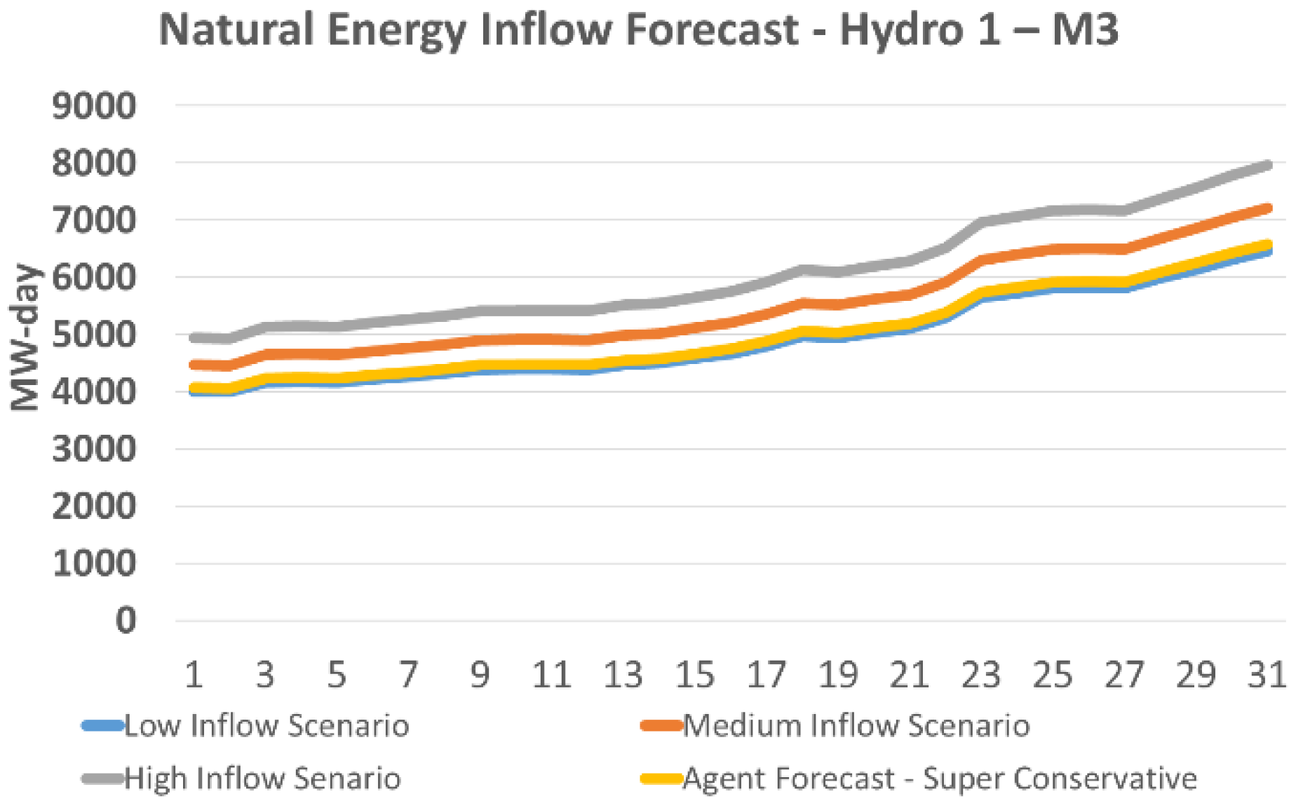
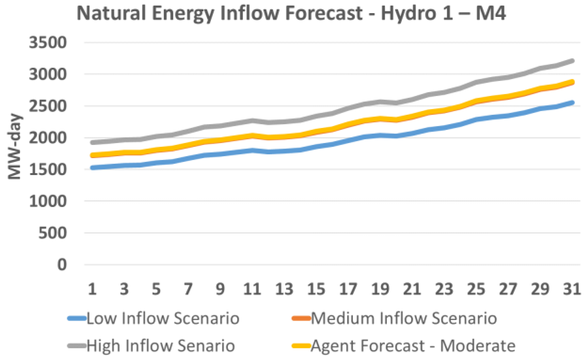
Below, the behavior of the initial forecast of the inflows that arrive at the reservoirs converted into energy, which is called natural energy inflow, is shown for the month under study. By way of illustration, the initial estimates for the first agent’s plant of each market is presented compared to the forecast made by the consulting company; it is worth noting that the behavior of the inflows of the plants of Agent 2 of each market would be very similar to the behavior of Agent 1 of each market illustrated in the Figure 5, Figure 6, Figure 7 and Figure 8.

As you can see, for 31 days, a super conservative agent assigns more weight to drier inflows than an agent with an aggressive profile that will predict wetter inflows. It is also worth noting that according to the market dynamics, during the simulations, the inflow forecast is updated by each agent, seeking to adapt to the “observed reality”.

Table 4 summarizes the operational data of the thermoelectric plants considered in the simulations. The type of fuel, the maximum and minimum generation and the cost of operation of each plant are presented.

In order to verify the effects of the variability in the generation of non-dispatchable renewable plants on the market demand and, consequently, on the market price, a wind farm was considered in Markets 2 and 3. In Market 2, it was considered a plant with an average generation forecast of 189 MWm, while in Market 3, it was 282 MWm. However, it is noteworthy that the generation of these plants in the simulations varies daily around the aforementioned averages. Finally, for simplicity, transmission limits between markets were not considered since the idea is to focus on the agent risk profile.

At the beginning of the month, each agent stipulates how the other hydraulic agents will behave.

Table 5. Agents’ risk profile—own and competitors’ view; source: own elaboration.

	View of Hydro 1–M1	View of Hydro 2–M1	View of Hydro 1–M2	View of Hydro 2–M2	View of Hydro 1–M3	View of Hydro 2–M3	View of Hydro 1–M4	View of Hydro 2–M4
Hydro 1–M1	Conservative	Conservative	Moderate	Conservative	Conservative	Conservative	Aggressive	Moderate
Hydro 2–M1	Conservative	Conservative	Conservative	Aggressive	Conservative	Conservative	Conservative	Moderate
Hydro 1–M2	Aggressive	Moderate	Aggressive	Moderate	Moderate	Moderate	Aggressive	Conservative
Hydro 2–M2	Aggressive	Aggressive	Moderate	Aggressive	Moderate	Moderate	Moderate	Conservative
Hydro 1–M3	Super conservative	Super conservative	Conservative	Super conservative	Super conservative	Conservative	Super conservative	Super conservative
Hydro 2–M3	Super conservative	Super conservative	Super conservative	Super conservative	Super conservative	Super conservative	Super conservative	Super conservative
Hydro 1–M4	Moderate	Moderate	Moderate	Super conservative	Conservative	Moderate	Moderate	Aggressive
Hydro 2–M4	Moderate	Conservative	Aggressive	Super conservative	Conservative	Moderate	Moderate	Moderate

presents the risk profile of each agent as well as the perception of the risk profile of competing hydroelectric agents.

Table 6. % final storage goals—own and competitors’ view; source: own elaboration.

	View of Hydro 1–M1	View of Hydro 2–M1	View of Hydro 1–M2	View of Hydro 2–M2	View of Hydro 1–M3	View of Hydro 2–M3	View of Hydro 1–M4	View of Hydro 2–M4
Hydro 1–M1	60%	60%	50%	65%	70%	65%	45%	60%
Hydro 2–M1	70%	60%	70%	45%	70%	65%	65%	60%
Hydro 1–M2	40%	55%	45%	55%	50%	50%	45%	70%
Hydro 2–M2	40%	55%	50%	45%	50%	50%	55%	70%
Hydro 1–M3	90%	85%	70%	80%	90%	75%	75%	80%
Hydro 2–M3	90%	85%	85%	80%	90%	90%	75%	80%
Hydro 1–M4	50%	60%	50%	80%	70%	50%	50%	40%
Hydro 2–M4	50%	70%	45%	80%	70%	50%	65%	50%

show the initial view of each agent in relation to the storage level at the end of the month given the risk profile; this forecast is made considering that the game month and the following have the behavior of presenting high inflows, but the profile risk of each can determine whether there will be more storage or not.

These behaviors can be changed during the competition over the weeks since it is possible that an agent, who judges a competitor as aggressive, observes a more moderate or conservative behavior and with that, changes his view of the competitor. As a premise, it is considered that all agents hold information from the system’s storage level and from other agents before the game and during the game, so it is possible for each agent to predict the competitors’ behavior.

5. Results and Discussion

Considering the assumptions described in the previous item, simulations of price bids and quantity of energy dispatched from eight agents were carried out during the 31 days of the first month of a given year. Each agent made its daily bids to the market operator based on its previous simulations of the market’s behavior, as is shown below. It is noteworthy, however, that the information provided by the market (inflows, demand, renewable generation) may differ from what each agent predicts; consequently, this causes the results to be different from those predicted by each agent. In addition, the acceptance of the bid may be different from what was expected since, at the time of the bidding, agents do not know the bidding amount and time of its competitor, and the real demand.

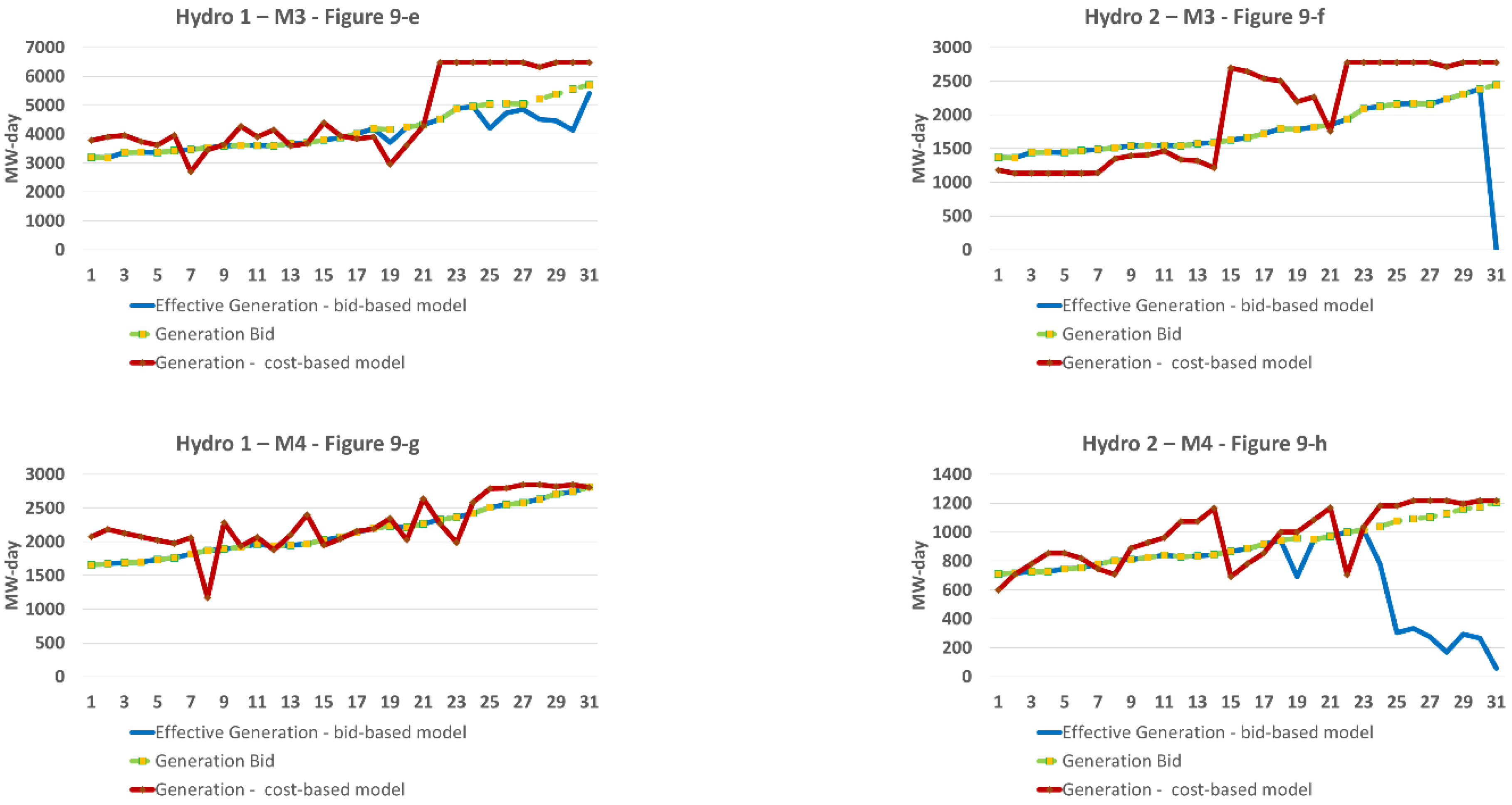
In this simulation, each agent presented the bids for the 31 days at the same time to the operator. Therefore, Figure 9a–h below (with captions grouped in Figure 9) illustrate the bids of the eight agents versus what was effectively dispatched (accepted) by the system operator if the average inflow occurred. In addition, the generation of the plants considering the determination of the dispatch by the operator from the minimum cost is also illustrated. As can be seen on certain days, in the bid model, some agents had the effective generation (blue line) that was different from the generation forecast at the beginning (generation bid in green dotted line) of the month. This occurs because, at the time of its bidding, the agent does not know what the biddings of its competitors are and the real demand.

Another aspect that can be observed is the variation in the behavior of the generation of the plants when compared to the one computed from a cost-based model. It is observed, for example, that the Hydro 1 generation has an inverse behavior between the simulations in the bid-based framework and in the cost-based model. This is due to the fact that the cost-based model does not take into account the plant’s conservative risk profile as well as the end-of-month storage target. As will be seen below, while Agent Hydro 1, when presenting its bid according to its strategy and risk, seeks to store water in the plant’s reservoir, in the cost-based model simulation, the reservoir ends up being more depleted (see Figure 10a later).

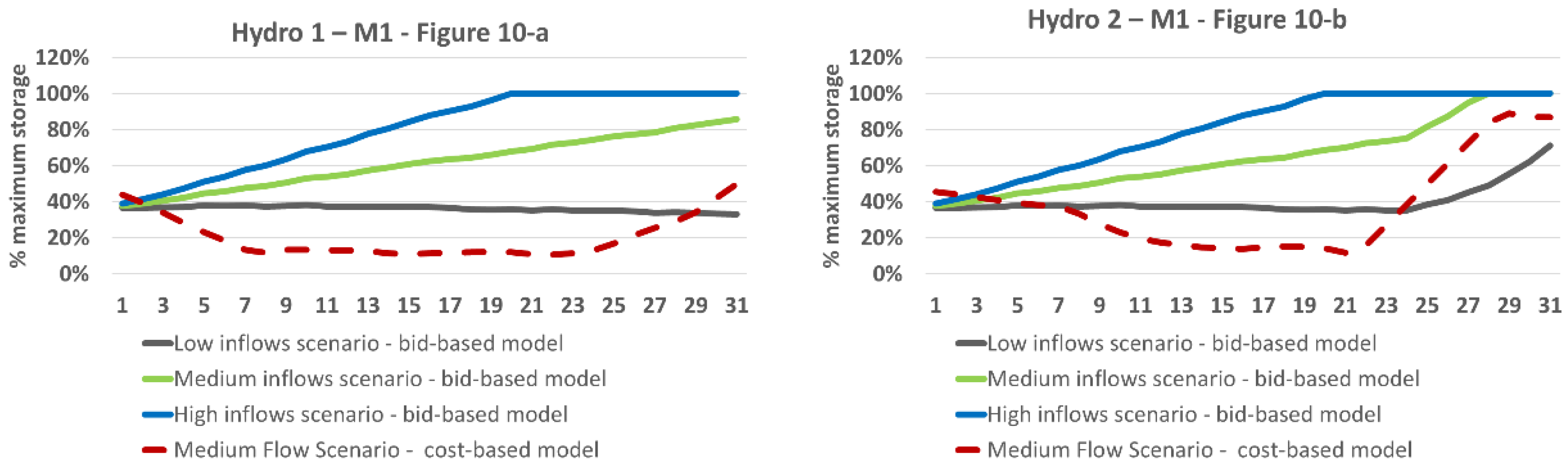
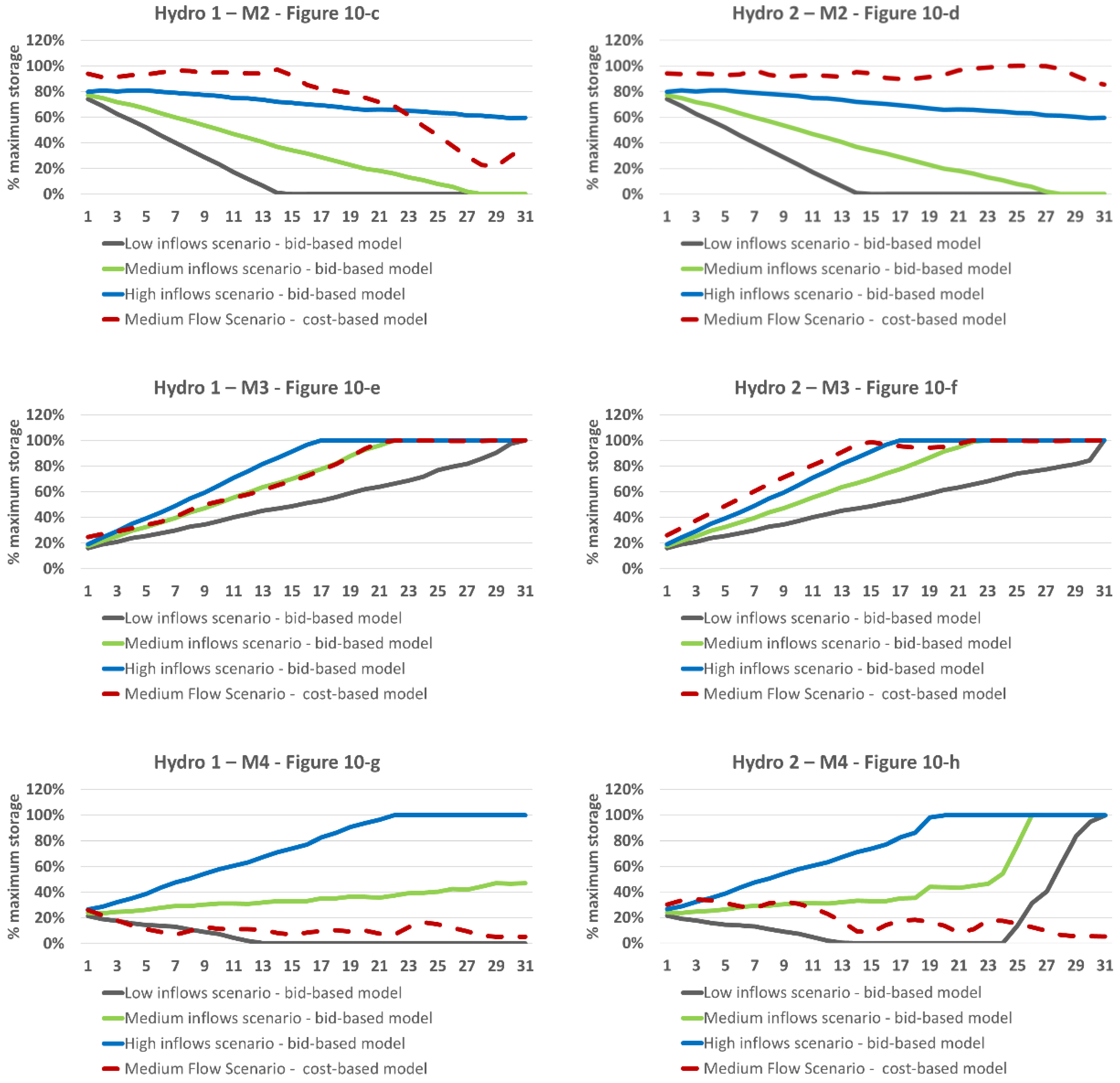
Figure 10a–h below (with captions grouped in Figure 10) present the behavior of storage for each hydraulic agent, in the bid simulations, considering the occurrence of three types of inflows: low, medium and high. The storage in the occurrence of the average flow in the simulation of the cost-based model is also presented. As you can see, in relation to the bid-based simulation, storage at the end of the month is completely different from the goals presented in Table 6 and the simulation results in the cost-based model. The reasons related to this variation are inflow rates and demands that are different from the forecast as well as the behavior of competitors that differed from the forecast of each agent. It is noteworthy that in these first simulations, each agent bid for 31 days without making any changes to the initial planning.

Regarding the simulations in the cost-based model, the difference comes from the operation policy promoted by the determination of a plant’s dispatch, which is different from the SOPEE that, still looking for a minimum cost for ordering/accepting bids, takes into account the generation proposal of each hydroelectric agent. The cost-based model chooses to operate more with the plants of Market 1 and 4, causing the reservoirs to reach minimum levels in a few days.

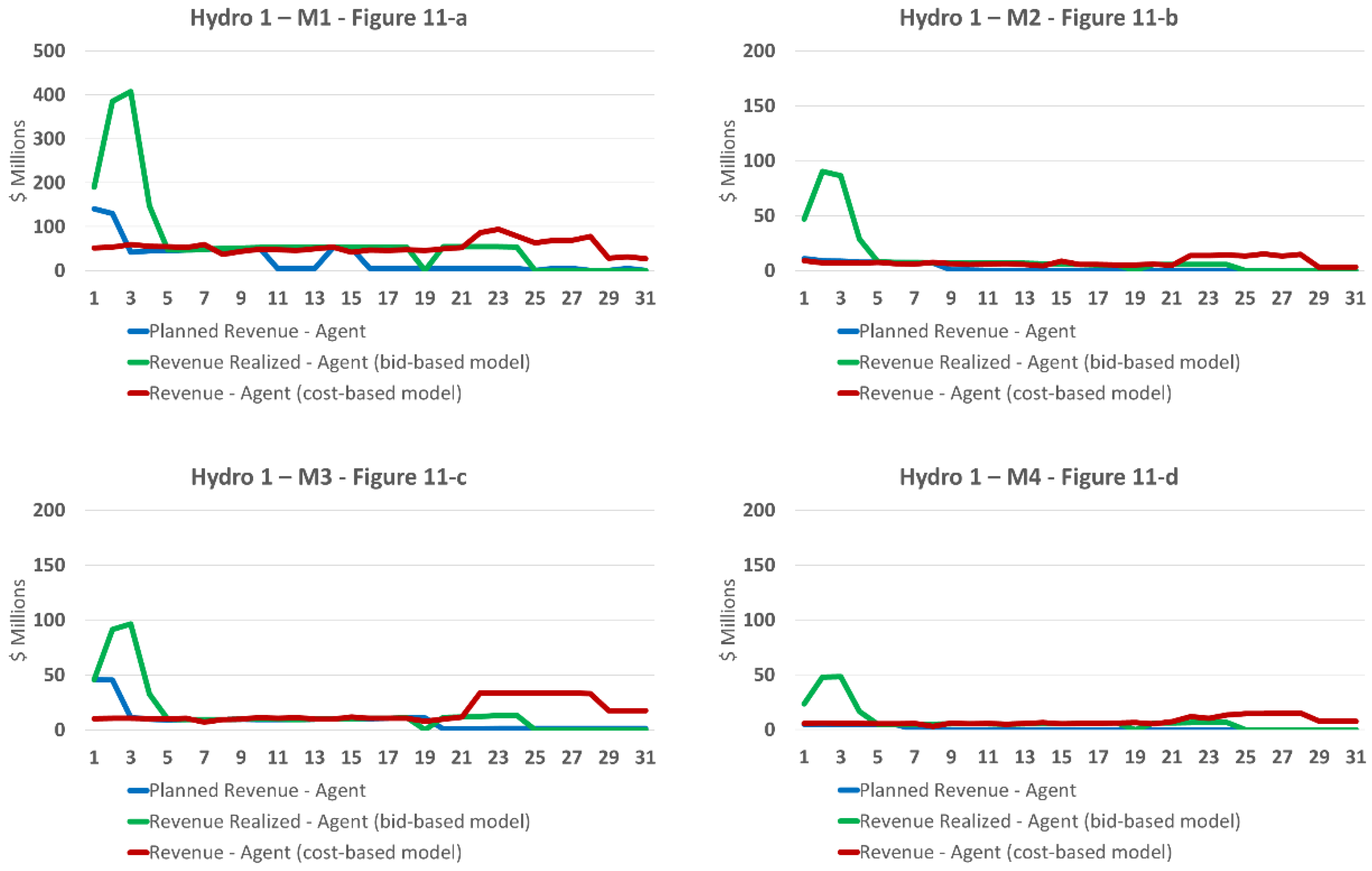
Figure 11a–d (with captions grouped in Figure 11) show a comparison of the behavior of the daily revenue of Agents 1 of each market, if the average inflow occurred. It is observed that, due to its generation and storage capacity, Agent 1 of Market 1–M1, is the one with the highest revenue (for better visualization of the results, it was decided to present the chart scale of Agent Hydro 1 of Market 1 (in Figure 11) that is different from the other agents), and has the greatest ability to influence the market. For example, if Hydro 1–M1 (Agent 1’s plant in Market 1) had an aggressive behavior, market prices would tend to be low, causing agents’ revenues to be low. This behavior can be observed in the simulation of the cost-based model where there is a predominant generation of Hydro 1 from Market 1. It can also be seen from the expectation of revenue from Agent 1 of Market 4–M4, which is quite low, compared to its realized revenue. This is because this agent expected an expressive generation from Hydro 1–M1 (because it has a moderate profile), estimating that only the cheapest thermal plant was activated to complement the demand. However, in reality, Hydro 1–M1 showed a more conservative behavior, generating less and resulting in an increase in market prices with the need for greater thermal complementation.

It is also observed that the revenues of all agents tend to be low after the first 7 days of the month; this is due to the large amount of water that reached the reservoirs. Therefore, considering the storage goals of each agent for the month, there was an excess in hydraulic supply to meet market demand.

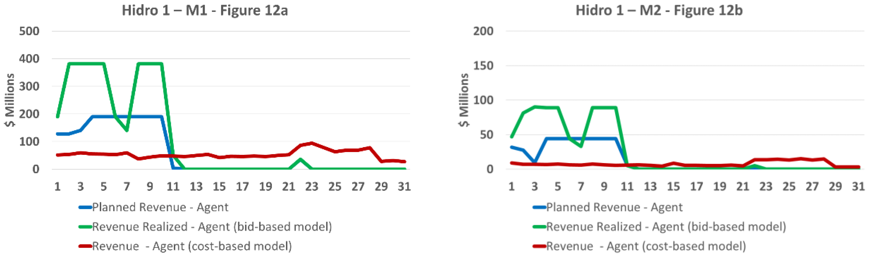
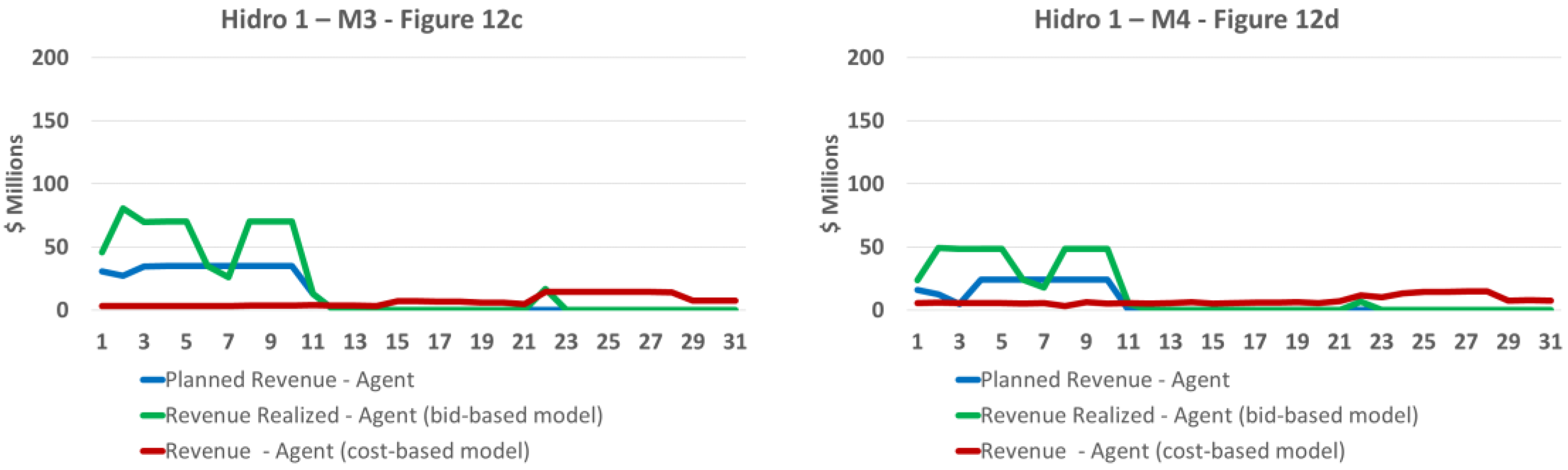
The previous results illustrated the behavior of the market if the game was considered with a view of monthly planning and storage goals for each agent, with the depletion or accumulation of water in the reservoirs being conducted daily until the goal for the month is reached. When sending the 31-day bid, the sensitivity of market variation is lost, considering only the reservoir target. Therefore, it is not a good strategy for an agent that wants to maximize revenue as it tends to have lower gains than if it were conducted with less granularity, as is shown below.

The next results shown in Figure 12a–d (with captions grouped in Figure 12) present an operation of the reservoirs with an evaluation and an expectation of reaching the reservoir goal every 10 days, seeking to reach the objective of the month. In this case, the agents update their expectation of inflow behavior and the generation bid of each agent. The behavior of the agents’ supply versus the effective generation is shown below.

Thus, it is observed how the strategy of filling and emptying the reservoirs, depending on the risk profile of an agent in a hydrothermal system, can influence the behavior of market prices. It is also observed the difficulties of predicting the agents’ behavior and the variables that influence prices, such as hydrology and the variation in renewable energy, even though estimation and parameter prediction tools are used.

However, it is possible to notice through

Table 7. Revenue planned vs. real in spot market; source: own elaboration.

	Revenue	Revenue— Case–Bid Each 31 Days		Revenue— Case–Bid Each 10 Days
	Cost-Based	Bid-Based		Bid-Based
	Real (USD Millions)	Planning (USD Millions)	Real (USD Millions)	Planning (USD Millions)	Real (USD Millions)
Hydro 1–M1	1666	826	2125	1767	3279
Hydro 1–M2	240	68	373	384	751
Hydro 1–M3	502	274	467	350	637
Hydro 1–M4	235	29	103	203	418

that compares the three simulations performed, that there is an increase in daily planned revenue when compared to the revenue presented for every day of the month at once. This is due to the daily refinement of agents’ perception of market behavior. At the same time, it is observed that the agents Hydro 1–M1 and Hydro 1–M2 have much higher revenues compared to the one obtained in the simulation of the cost-based model. On the other hand, revenues for agents Hydro 1–M3 and Hydro 1–M4 are higher for the simulation of the cost-based model.

It is also worth noting that the simulations performed were performed interactively using a simulator that emulates the system’s operation with the bids presented by the agent according to its risk perception, which was refined according to the observation of market signals. It can be said that this is the way to reach the CE, requiring a large number of simulations for the best refinement to achieve the best reward. It is understood that this prior refinement with greater precision and speed could be easily achieved with algorithms related to artificial intelligence related to reinforcement learning.

In this sense, an iterative process can be suggested, through an algorithm, for the calculation of the CE that would consist of:

In each period, the agent conducts a retrospective analysis to decide whether to continue submitting the same bid as in the previous period, or switch to other bids, with probabilities that are proportional to how much higher his accrued revenue would be if he had always made that change in the past.

More precisely, let U be your accumulated revenue so far; and for each bid k different from his bid j from the last period, let V(k) be his cumulative revenue if he had submitted bid k every time he chose bid j (all else being unchanged). Then, only those bids k where V(k) is greater than U can be considered for exchange, with probabilities that are proportional to the difference V(k)-U, which is called “regret” for having submitted “j” instead of “k”. These probabilities can be normalized by a fixed factor so that their sum is strictly less than 1. With the remaining probability, the same bid “j” is chosen as in the last period. This proposed approach was based on [43] where it can be seen in more detail.

An interesting aspect that can be observed through the algorithm is that as it converges, the “regret” trends toward zero, and with that, every bid exchange function implies, in the end, a loss of revenue. (Note that in each period of the algorithmic simulations, the agent has to save the bid of its opponents in the previous periods to calculate its revenue if it had changed bids. In a second article, Hart and Mas-Collel [58] proposed an extension of the algorithm in which this information is not needed. In this extension, the agent only needs to keep the revenues and probabilities of bids in the past periods.) That is, CE is compatible with minimizing regret in hindsight. Thus, in view of the statement above, it is suggested as future work, for this same market configuration, to use the correlation with machine learning by reinforcement to reduce regret by defining the best strategy.

6. Conclusions

In the present article, the behavior of hydroelectric agents was evaluated in a competitive energy market with a characteristic of a hydrothermal generation system and little participation of non-conventional renewables (wind).

The study reflected qualitative and quantitative examples of how the perception and behavior of each agent can influence market behavior. In this case, it is important to point out that it was possible to verify the influence of the perception of the parameters that form the energy price. The results showed that the market behavior, if the game was considered with a monthly planning vision and storage goals for each agent, instead of planning every 10 days, tends to have lower gains, demonstrating the importance of greater granularity and pari passu monitoring of the market to define and redefine bid strategies since it is expected to increase revenue and minimize regret due to the daily refinement of the agents’ perception.

With the highest level of uncertainty in the energy market, the risk profile of each agent has a considerable influence on the supply strategy, as in a financial market. In addition, in the present study, it was possible to observe how much the risk profile of competing agents can influence the bids of each agent. In this sense, the profile directly influences the view of the parameters that affect the market price, such as hydrology and the availability of hydraulic supply, as well as the generation of renewable energy, and the demand and bids of competitors. An agent with a lot of influence in the market, depending on its profile, can bring about significant variations in market behavior, so it is important that each agent observes its behavior to define bids.

At the same time, it was also possible to observe how the results of the simulations in the bid-based model were quite different from those obtained through the simulations in the cost-based model. This occurs because while in the bid-based model agents make their decision seeking to maximize their profits, in the cost-based model, the decision to generate energy, in which consequent market price formation is based, is guided around the best use of the generation sources as well as the minimization of the cost of energy production. Therefore, the observed differences are directly connected to the objective, the perception of the parameters that form the price (directly linked to the risk profile) and the participation of each agent in the market.

Finally, it should be noted that the study complements solutions previously presented in the literature, as mentioned throughout the article, in order to contribute to improvements in the definition of optimal energy bids, especially in a hydrothermal system that has a high level of uncertainty. However, due to the intentional simplifications considered, the correlation with machine learning by reinforcement is suggested as future work, for this same market configuration, because it is believed that the robustness of the machine learning technique for data mining tasks, can be great for finding and adjusting agent bid patterns, and one could reduce regret by defining the best strategy.