An Improved Frequency-Adaptive Virtual Variable Sampling-Based Repetitive Control for an Active Power Filter

Abstract

To eliminate the harmonics caused by nonlinear loads, repetitive controllers are widely applied as current controllers for active power filters (APF). In practice, a variation in grid frequency leads to the appearance of a fractional-order delay filter. As a result, the resonant frequency of the repetitive controller will deviate from the fundamental frequency and the controller cannot compensate for harmonics accurately. To solve this problem, an improved frequency-adaptive repetitive controller based on virtual variable sampling (IMFA-VVS-RC) for APF is proposed in this paper. To enhance the system stability margin, the proposed RC introduces an infinite impulse response (IIR) low-pass filter. The proposed RC has a high stability margin at high frequencies due to the low gain of the IIR low-pass filter in the region above the cutoff frequency. In this way, the influence of model uncertainty and parameter uncertainty on system stability are reduced at high frequencies. At the same time, compared with the conventional repetitive controller (CRC), the proposed RC for APF has a better harmonic suppression ability when the frequency varies. Experiments have verified the effectiveness of the scheme adopted for APF.

1. Introduction

In recent years, the demand for new energy such as wind power and hydropower has been increasing day by day. As a result, a large number of nonlinear loads using switching devices are connected to the power grid, such as rectifiers and grid-connected inverters [1]. The currents flowing through nonlinear loads are not sinusoidal, so many harmonics are injected into the grid, which affects the stability and safety of the power system. To deal with this problem, the APF is widely used in harmonic compensation because of its small size and low resonance [2,3,4,5,6,7,8].

In the application of the APF, the selection of the current controller can be crucial. The proportional–integral (PI) controller has a simple structure, is easy to adjust, and has strong robustness. As a result, it has become one of the most widely used controllers. However, according to the internal model principle proposed by Inoue in 1981 [9], since the internal model only contains a DC signal, the PI controller cannot track the periodic signal without steady-state error. Therefore, it is necessary to perform complex Park’s transformation and convert it into a DC signal on the synchronous rotating coordinate system. The proportional–resonant (PR) controller has infinite gain at a specific frequency and can control a periodic signal at that frequency without steady-state error. In the use process, multiple PR controllers need to be connected in parallel and the parameter design is complicated. Therefore, it is difficult to guarantee system stability.

The internal model of the CRC contains periodic signals, and the CRC is widely used for APF in tracking periodic signals without error [10,11,12,13,14,15,16]. As a result, it can be applied to tracking the fundamental wave and multiple specific frequency harmonics. The CRC is realized by an N-order delay filter $z^{-N}$, where $N=f_s/f_r$. $f_s$ stands for sampling frequency and $f_r$ stands for the fundamental frequency of the reference signal (or grid frequency). When the grid frequency is normal, N is kept as an integer, and CRC can compensate for harmonics well. However, in actual situations, the ratio N cannot remain an integer because of the variation in grid frequency $f_r$. The fractional-order delay filter cannot be realized digitally, so the nearest integer is generally taken. This approximation leads to the deviation of resonant frequencies from the reference fundamental frequencies and harmonic frequencies [17,18,19,20,21,22]. Therefore, the gain of CRC at the resonant frequencies is greatly reduced. This affects the harmonic rejection capability of the CRC.

To deal with this problem, a great deal of research has been conducted on frequency-adaptive repetitive controllers (FARCs). One method is to increase the gain of the controller at the resonant frequency. A scheme that introduces a correction factor has been proposed [23,24]. This scheme can bring the resonant frequency close to the fundamental and harmonic frequencies. However, its limitation is the need to design parameters for multiple controllers in parallel. The difficulty of parameter design is increased. Another method is to solve the problem of N being a fraction. When the grid frequency varies, the ratio N can be kept constant by changing the sampling frequency accordingly. For this purpose, a variable sampling technique based on a phase sampling circuit has been developed [25,26,27]. The phase sampling circuit can sample at every fixed phase interval $\Delta \theta$, where $\Delta \theta =2\pi /N$. However, the additional circuit increases the complexity of the system, and the variable sampling frequency is not conducive to hardware implementation. In order to ensure that this method can be implemented in hardware, a fixed sampling frequency is required. A frequency-adaptive variable virtual sampling (VVS) technique for grid-connected inverters has been proposed [28,29]. This technique enables the use of a variable sampling frequency with virtual delay filters. Virtual delay filters are composed of integer-order delay filters in the form of polynomials. In this way, hardware implementation can be accomplished due to the use of a fixed sampling frequency.

In this paper, an improved frequency-adaptive repetitive controller based on VVS (IMFA-VVS-RC) is proposed. On the basis of the controller based on VVS technique, an infinite impulse response (IIR) low-pass filter is added to enhance the robustness of the system. At the same time, the variation of the resonant frequencies due to the IIR filter is successfully eliminated by changing the virtual sampling frequency. The IIR low-pass filter can enhance the stability margin of the system at a high frequency due to its low gain at high frequencies. Compared with the FIR filter, the IIR filter possesses better high-frequency attenuation characteristics. In this way, the frequency range at which the system is stable is widened. Moreover, the influence of model uncertainty and parameter uncertainty are attenuated at high frequencies, mainly including changes in inductance and capacitance in the LCL filter. The parameter robustness of the proposed controller is enhanced. This paper selects the Butterworth filter as the IIR filter, which satisfies the maximally flat criterion. The VVS scheme is applied to the repetitive controller of the single-phase APF system because of its frequency-adaptive characteristics.

The rest of this paper is organized as follows. Section 2 illustrates the functioning and drawbacks of the CRC. This section mainly describes the variation of resonant frequency when the power grid frequency varies. In Section 3, a detailed discussion of the VVS technique is provided and the VVS technique is applied to IMFA-VVS-RC. The stability criteria and the harmonic suppression capability of the proposed RC are analyzed. In Section 4, the parameter of the proposed RC is designed. In Section 5, the IMFA-VVS-RC is used for LCL-type APF and the control structure is designed. The experiments mainly compare the harmonic suppression capability of the proposed RC and the CRC. At the same time, the dynamic characteristics of the proposed RC under parameter changing and load changing conditions are verified. The conclusion is given in Section 6.

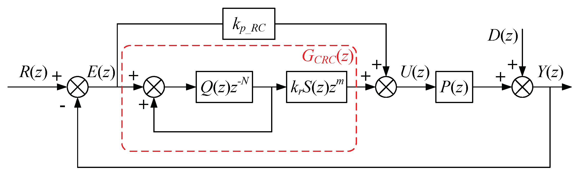
2. Conventional Repetitive Controller

CRC is typically used in plug-in form. Figure 1 shows the close-loop plug-in CRC control system, where $R\left(z\right)$ is the reference input, $Y\left(z\right)$ is the output of closed-loop system, and $U\left(z\right)$ is the output of the controller. $E\left(z\right)=R\left(z\right)-Y\left(z\right)$ is the tracking error and $D\left(z\right)$ is the disturbance. $P\left(z\right)$ is the plant. $G_{CRC}\left(z\right)$ is the CRC controller and $k_{p\_RC}$ is the proportional gain of the plug-in system. In the CRC structure, $Q\left(z\right)$ is the low-pass filter, where $Q\left(z\right)={\alpha }_{1}z+{\alpha }_0+{\alpha }_1{z}^{-1}$, $2{\alpha }_{1}z+{\alpha }_0=1$. $k_r$ is the RC gain and $z^m$ is the phase lead compensation filter. $S\left(z\right)$ is the compensator, which is used to compensate for the magnitude response of the controller to unity.

According to Figure 1, the transfer function of the CRC in the control system can be expressed as (1).

$$G_{CRC}\left(z\right)=k_r\frac{z^{-N}Q\left(z\right)}{1-z^{-N}Q\left(z\right)}S\left(z\right)z^m$$

(1)

Consider that, without $Q\left(z\right)$, CRC can provide infinite gain at a fundamental frequency and harmonic frequencies. As a result, the harmonics can be compensated exactly by the controller. However, in the actual situation, the performance of the CRC is sensitive to the grid frequency variation. As shown in Figure 2, for $k_r=15$, $Q\left(z\right)=0.1z+0.8+0.1z^{-1}$, $m=3$, and $S\left(z\right)=1$, obtaining a magnitude response in the range of 10 Hz–680 Hz. When the reference fundamental wave frequency varies in the range of 50 ± 1 Hz, the variation range of the nth harmonic is $n(50\pm 1)$ Hz. As shown in the little picture in Figure 2, the magnitude response curve at around 150 Hz can be obtained by locally magnifying the 3rd resonant frequency. When the frequency varies from 150 Hz to 150 ± 3 Hz, the CRC gain decreases from 83.3 dB to 32.0 dB. In the same way, when the frequency varies from 350 Hz to 350 ± 7 Hz, the CRC gain decreases from 69.8 dB to 24.9 dB. Thus, the higher the frequency is, the farther the frequency will vary from the resonant frequency. As a result, the the gain drop at the reference harmonic frequency will be greater. Therefore, the CRC’s capability to suppress the harmonics of these frequencies deteriorates.

3. Improved Frequency-Adaptive Repetitive Controller

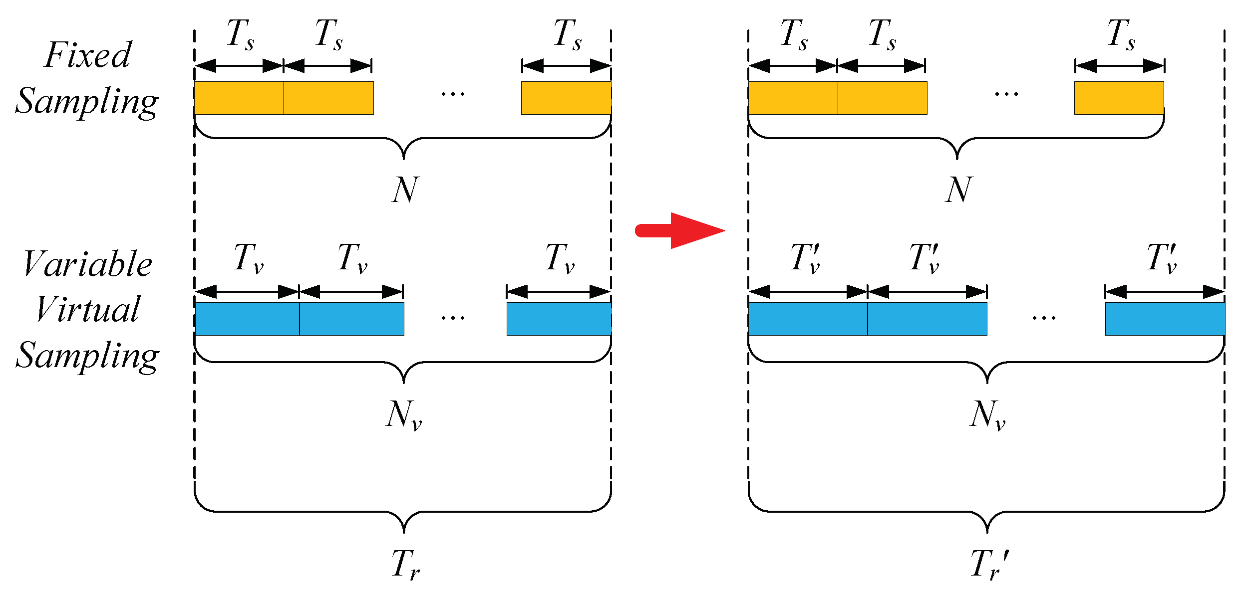
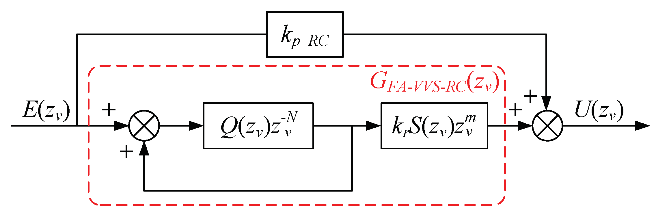
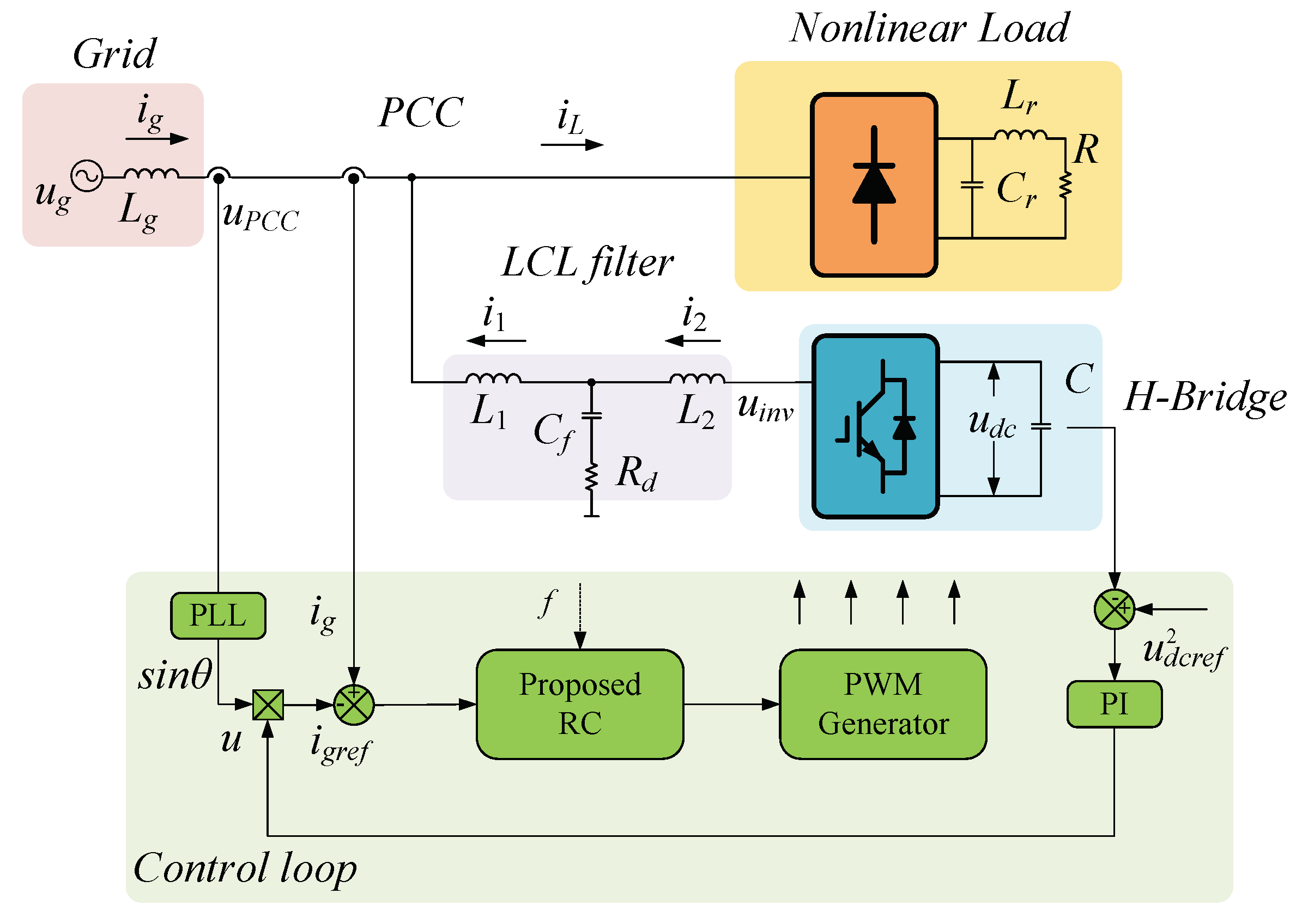
3.1. Description of Control Scheme

The variable virtual sampling delay filter can eliminate the fractional-order delay filter caused by frequency variation. As shown in Figure 3, the variable virtual sampling period $T_v$ will change accordingly when the reference signal period changes from $T_r$ to $T_r^{{}^{\prime }}$. The VVS period $T_v$ can be obtained by $T_v=T_r/N_v$. As a consequence, the ratio $N_v$ will remain an integer and the control scheme becomes realizable. In contrast, the period $T_s$ of the fixed sampling scheme cannot be adjustable, which will cause errors.

A polynomial composed of fixed sample delay filters $z^{-1}$ (including $z^{-1}$, $z^{-2}$,…, $z^{-n}$) is used to represent a variable virtual sample delay filter $z_v^{-1}$. To make a trade-off between the approximation accuracy and the system complexity, select n as 3. As shown in (2), the polynomial coefficients $x_i$ are calculated via the Lagrange interpolation method. The polynomial coefficients change accordingly when the grid frequency varies. In this way, frequency adaptation is added to the sampling process.

$$z_v^{-1}=\sum _{i=1}^n{x}_i{z}^{-i},\mathrm{with}{x}_i=\prod _{j=1,j\ne i}^n\frac{T_v-j{T}_s}{i{T}_s-j{T}_s}$$

(2)

Figure 4 shows the IMFA-VVS-RC system with a plug-in structure. By applying the virtual sampling delay filter to RC and combining it with (1), the open-loop transfer function of IMFA-VVS-RC can be obtained.

$$G_{IMFA-VVS-RC}\left(z_v\right)=\frac{k_r{z}_v^{-N_v}Q\left(z_v\right)}{1-z_v^{-N_v}Q\left(z_v\right)}S\left(z_v\right)z_v^m$$

(3)

In s-domain, (4) can be expressed as:

$$\begin{array}{cc}\hfill G_{IMFA\_-VVS-RC}\left(s\right)& =\frac{k_r{e}^{-T_{r}s}Q\left(s\right)}{1-e^{-T_{r}s}Q\left(s\right)}S\left(s\right)e^{m{T}_{v}s}\hfill \\ & =k_r{G}_{RC}\left(s\right)S\left(s\right)e^{m{T}_{v}s}\hfill \\ \hfill \end{array}$$

(4)

By considering $G_{RC}$, (5) can be obtained.

$$\begin{array}{cc}\hfill G_{RC}\left(s\right)& =\frac{e^{-T_{r}s}Q\left(s\right)}{1-e^{-T_{r}s}Q\left(s\right)}\hfill \\ & =\frac{e^{-(T_{r}s-lnQ\left(s\right))}}{1-e^{-(T_{r}s-lnQ\left(s\right))}}\hfill \\ \hfill \end{array}$$

(5)

In favor of linearization, a first-order Taylor expansion of $Q\left(s\right)$ is performed at the origin, and the remainder is ignored.

$$lnQ\left(s\right)\approx lnQ\left(0\right)+\frac{Q^{\prime }\left(0\right)}{Q\left(0\right)}s$$

(6)

According to [30], the transfer function can be expanded as:

$$\begin{array}{cc}\hfill G_{RC}\left(s\right)& \approx \frac{e^{-\left[T_r-Q^{\prime }\left(0\right)/Q\left(0\right)\right]s+lnQ\left(0\right)}}{1-e^{-\left[T_r-Q^{\prime }\left(0\right)/Q\left(0\right)\right]s+lnQ\left(0\right)}}\hfill \\ & \approx -\frac{1}{2}+\frac{1}{(1-\gamma )T_r}\frac{1}{s-\frac{lnQ\left(0\right)}{(1-\gamma )T_r}}+\frac{2}{(1-\gamma )T_r}\sum _{k=1}^{\infty }A\left(k\right)\hfill \\ \hfill \end{array}$$

(7)

In (7), $A\left(k\right)$ can be expressed as:

$$A\left(k\right)=\frac{s-\frac{lnQ\left(0\right)}{(1-\gamma )T_r}}{{\left(s-\frac{lnQ\left(0\right)}{(1-\gamma )T_r}\right)}^2+{\left(k\frac{2\pi }{(1-\gamma )T_r}\right)}^2}$$

(8)

where $\gamma =Q^{\prime }\left(0\right)/\left[Q\left(0\right)T_r\right]$. According to (7) and (8), it can be deduced that resonant frequencies are deviated to $k{f}_r/(1-\gamma )$ by the inverse Laplace transform. The deviation of resonant frequencies is attributed to the introduction of the IIR low-pass filter.

To compensate for the deviation of the resonant frequency, a delay filter $e^{-\gamma T_{r}s}$ is introduced into the transfer function $G_{RC}\left(s\right)$. The transfer function $G_{RC}^{\prime }\left(S\right)$ in s-domain after compensation is shown in (9). Similar to the derivation process from (3) to (8), the resonant frequencies can be deduced back to $f_r$.

$$G_{RC}^{\prime }\left(s\right)=\frac{e^{-(1+\gamma )T_{r}s}Q\left(s\right)}{1-e^{-(1+\gamma )T_{r}s}Q\left(s\right)}$$

(9)

Convert (9) to z-domain, (10) can be obtained.

$$G_{IMFA-VVS-RC}\left(z_v\right)=\frac{k_r{z}_v^{-(N_v+\beta )}Q\left(z_v\right)}{1-z_v^{-(N_v+\beta )}Q\left(z_v\right)}S\left(z_v\right)z_v^m$$

(10)

where $\beta =\gamma T_r/T_v$. $\beta$ may be a fraction, making the proposed RC unrealizable. Change the virtual sampling frequency from $T_v$ to $T_{v1}$, where $T_{v1}=T_v(\beta +N_v)/N_v$. So (11) can be obtained.

$$\begin{array}{c}\hfill \frac{T_r}{T_{v1}}=\frac{T_r}{\frac{\beta +N_v}{N_v}{T}_v}=\frac{\frac{T_r}{T_v}}{\frac{\beta +N_v}{N_v}}=\frac{\beta +N_v}{\frac{\beta +N_v}{N_v}}=N_v\end{array}$$

(11)

As described in (12), the fractional-order delay filter $z_v^{-(N_v+\beta )}$ caused by the IIR low-pass filter is eliminated by changing the virtual sampling period(frequency). $z_{v1}^{-1}$ is a delay filter whose virtual sampling frequency changes to $T_{v1}$. By replacing the $z_v^{-1}$ in (3) with $z_{v1}^{-1}$, the relation (12) can be deduced.

$$G_{IMFA-VVS-RC}\left(z_{v1}\right)=\frac{k_r{z}_{v1}^{-N_v}Q\left(z_{v1}\right)}{1-z_{v1}^{-N_v}Q\left(z_{v1}\right)}S\left(z_{v1}\right)z_{v1}^m$$

(12)

By changing the virtual sampling frequency, the influence of the introduction of an IIR low-pass filter on the resonant frequency is successfully eliminated. Therefore, the transfer function of the proposed RC can be realized digitally.

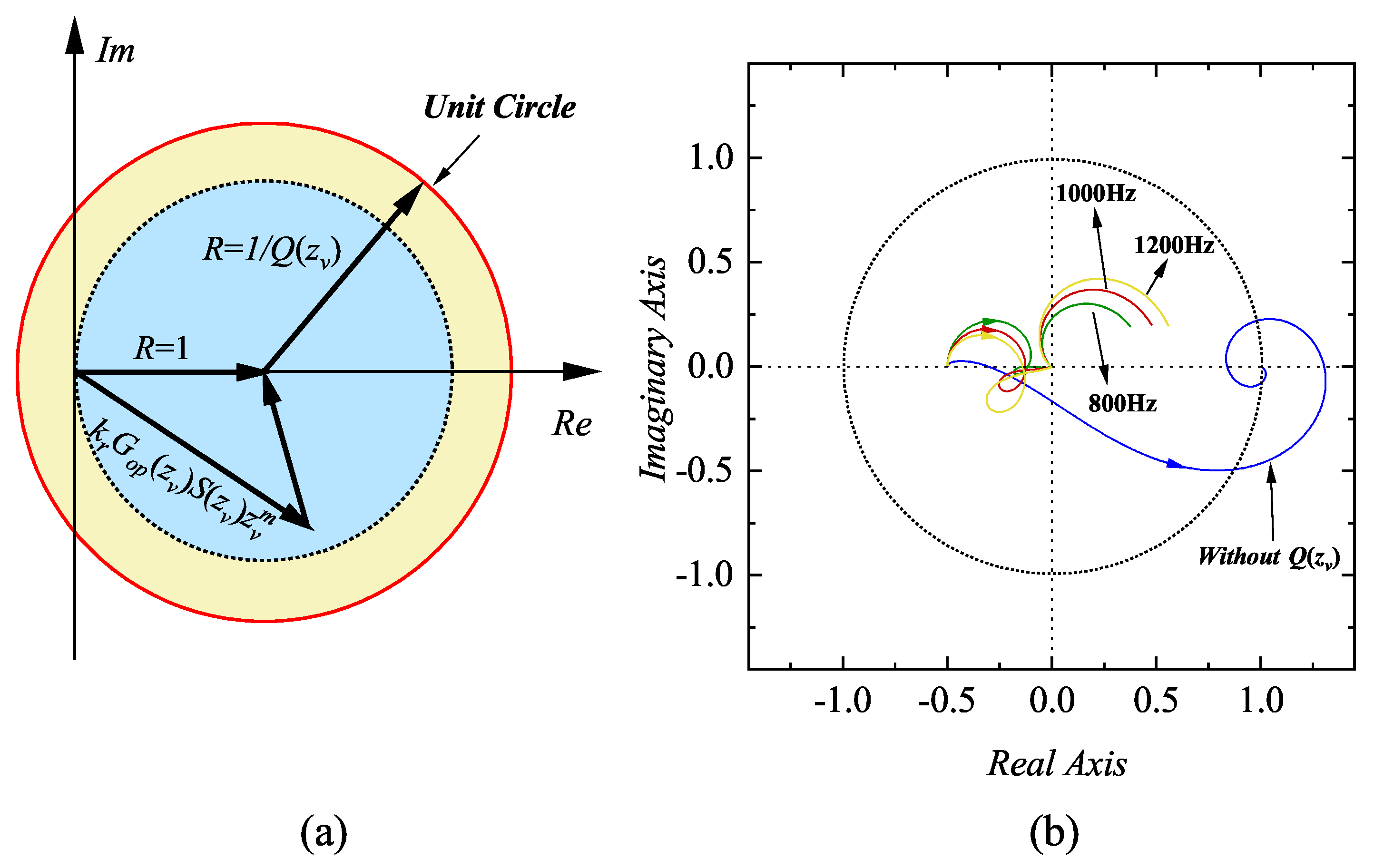
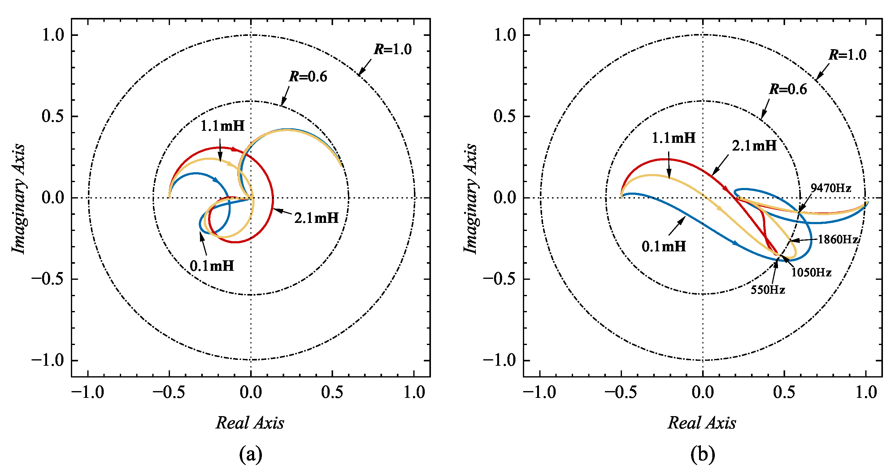
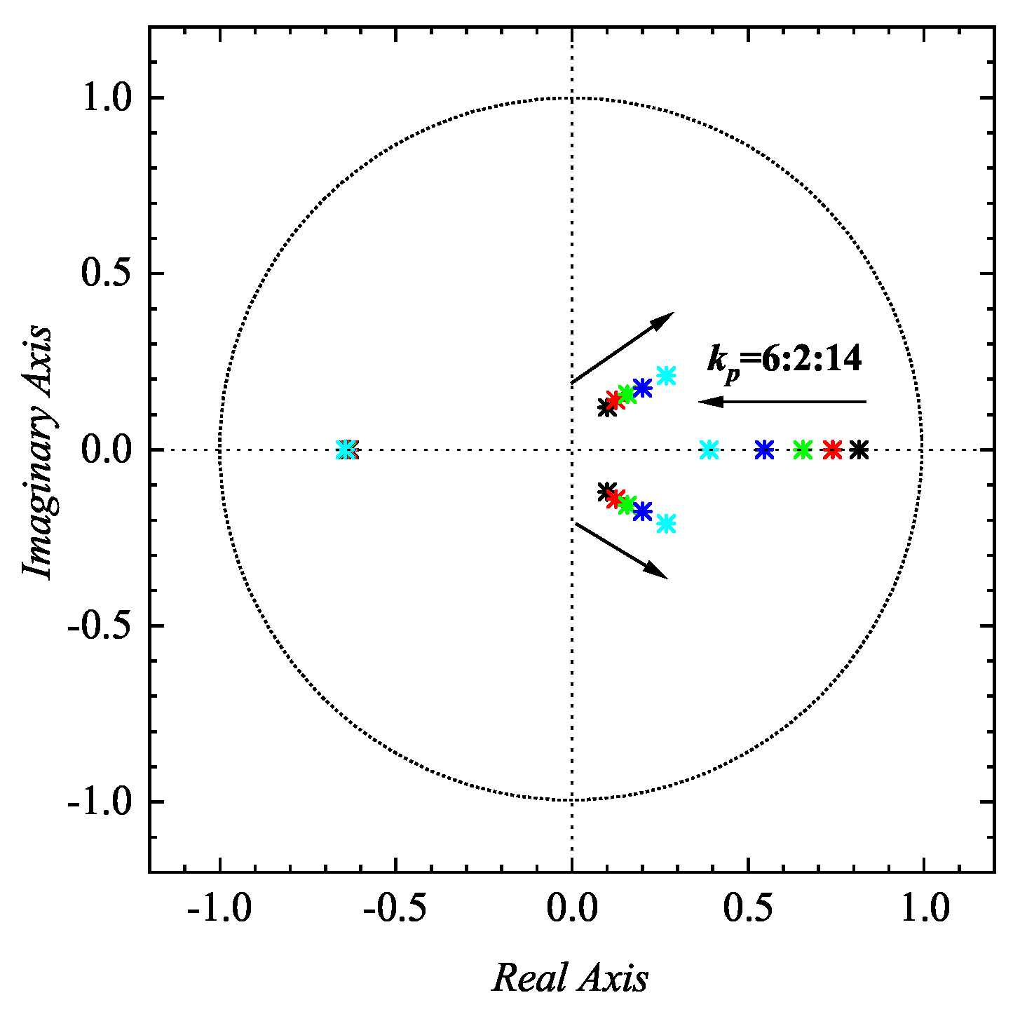
3.2. Stability Analysis

In order to verify the influence of IIR low-pass filter $Q\left(z_{v1}\right)$ on the stability margin, the stability criteria of the system needs to be derived. The stability criteria are obtained from the system characteristic equation, which needs to be derived later.

Considering the feedback loop, the closed-loop transfer function of the system can be obtained as (13):

$$G_{loop}\left(z\right)=\frac{[k_{p\_RC}+G_{IMFA-VVS-RC}\left(z_{v1}\right)]P\left(z\right)}{1+[k_{p\_RC}+G_{IMFA-VVS-RC}\left(z_{v1}\right)]P\left(z\right)}$$

(13)

where $1+[k_{p\_RC}+G_{IMFA-VVS-RC}\left(z_{v1}\right)]P\left(z\right)$ is the system characteristic polynomial, which can be expressed as:

$$[1+k_{p\_RC}P\left(z\right)][1+G_{IMFA-VVS-RC}\left(z_{v1}\right)G_p\left(z\right)]$$

(14)

In (14), $G_p\left(z\right)$ represents:

$$G_p\left(z\right)=\frac{P\left(z\right)}{1+k_{p\_RC}P\left(z\right)}$$

(15)

According to the characteristic polynomial, the system is stable when the characteristic polynomial satisfies the following two conditions.

• $1+G_{IMFA-VVS-RC}\left(z_{v1}\right)G_p\left(z\right)\ne 0$.
• The roots of $1+k_{p\_RC}P\left(z\right)=0$ are all inside the unit circle.

Substituting (3) and (15) into $1+G_{IMFA-VVS-RC}\left(z_{v1}\right)G_p\left(z\right)\ne 0$, we can obtain the following equations:

$$\left|1-Q\left(z_{v1}\right)z_{v1}^{-N_v}+k_{r}Q\left(z_{v1}\right)z_{v1}^{-N_v}S\left(z_{v1}\right)z_{v1}^m{G}_p\left(z\right)\right|\ne 0$$

(16)

(16) can be satisfied if:

$$\left|1-k_r{G}_p\left(z\right)S\left(z_{v1}\right)z_{v1}^m\right|<\frac{1}{\left|Q\left(z_{v1}\right)\right|}$$

(17)

Adding a IIR low-pass filter $Q\left(z_{v1}\right)$ changes the right-hand side of the Equation (17) from 1 to $1/Q\left(z_{v1}\right)$. When the frequency is upper than the IIR low-pass filter cutoff frequency, the magnitude of the IIR low-pass filter decreases considerably. As a result, the right-hand side of the Equation (17) increases dramatically. We define the following formula:

$$T\left(z\right)=Q\left(z_{v1}\right)\left|1-k_r{G}_p\left(z\right)S\left(z_{v1}\right)z_{v1}^m\right|$$

(18)

Some symbols are defined as follows:

• $S\left(z_{v1}\right)=N_s\left(\omega \right)exp\left[{\theta }_s\left(\omega \right)\right]$
• $G_p\left(z\right)=N_g\left(\omega \right)exp\left[{\theta }_g\left(\omega \right)\right]$
• $Q\left(z_{v1}\right)=N_q\left(\omega \right)exp\left[{\theta }_q\left(\omega \right)\right]$

where $N_s\left(\omega \right)$, $N_g\left(\omega \right)$, and $N_q\left(\omega \right)$ are the magnitude responses of $S\left(z_{v1}\right)$, $G_p\left(z\right)$, and $Q\left(z_{v1}\right)$, respectively, and ${\theta }_s\left(\omega \right)$, ${\theta }_g\left(\omega \right)$, and ${\theta }_q\left(\omega \right)$ are the phase responses of $S\left(z_{v1}\right)$, $G_p\left(z\right)$, and $Q\left(z_{v1}\right)$, respectively. According to Euler’s formula, the stability criterion of the plug-in IMFA-VVS-RC system can be obtained.

$$\begin{array}{cc}\hfill 0<k_r& <\frac{1-N_q^2\left(\omega \right)}{k_r{N}_q^2\left(\omega \right)N_s^2\left(\omega \right)N_g^2\left(\omega \right)}\hfill \\ \hfill & +\frac{2cos({\theta }_g\left(\omega \right)+{\theta }_s\left(\omega \right)+m\omega )}{N_g\left(\omega \right)N_s\left(\omega \right)}\hfill \\ \hfill \end{array}$$

(19)

According to Figure 5, the influence of $Q\left(z_{v1}\right)$ on the stability margin can be quantitatively analyzed in the form of vectors and Nyquist curves. The IIR low-pass filter can be expressed as (20):

$$Q\left(z_{v1}\right)=\frac{{\displaystyle \sum _{k=0}^n}{\alpha }_k{z}_{v1}^{-k}}{1+{\displaystyle \sum _{k=1}^n}{\beta }_k{z}_{v1}^{-k}}$$

(20)

As shown in Figure 5a, in order to enhance the stability of the system, an IIR low-pass filter is added to the proposed RC. At low and medium frequencies, the system model can be established and compensated accurately. The end of $k_r{G}_p\left(z\right)S\left(z_{v1}\right)z_{v1}^m$ is close to (1, 0), and the left side of (17) is inside the unit circle (blue circle). Thus, the system stability criterion can be satisfied and it is similar to the situation when $Q\left(z_{v1}\right)=1$. At high frequencies, the magnitude of $1/Q\left(z_{v1}\right)$ (yellow circle) increases and the stability margin of the system grows larger. Thus, the influence of parameter uncertainty on the system stability is solved to a certain extent.

Figure 5b specifically illustrates the influence of IIR low-pass filter $Q\left(z_{v1}\right)$ on system stability at high frequencies. The variation trend of $T\left(z\right)$ with the cutoff frequency of the filter is also shown. When the IIR low-pass filter is introduced, the Nyquist curve of the $T\left(z\right)$ is all inside the unit circle. On the contrary, in the absence of an IIR low-pass filter, the Nyquist curve is outside the unit circle at high frequencies. As the cutoff frequency of the IIR rises from 800Hz to 1200Hz, the Nyquist curves of the $T\left(z\right)$ gradually approach the unit circle, leading to a decrease in the stability margin.

As shown in Figure 6a,b, when the grid-side inductance varies from 0.1 mH to 2.1 mH, the Nyquist curves are close to the unit circle at low frequencies and vary slightly at high frequencies. Figure 6a,b adopt a Butterworth filter with cutoff frequency of 1200 Hz and a zero-phase-shift FIR filter $Q\left(z_{v1}\right)=0.2z_{v1}+0.6+0.2z_{v1}^{-1}$, respectively. Comparing Figure 6a,b, the IIR filter can restrict the Nyquist curves to a circle with $R=0.6$, so the stability margin can be defined as $1/R=1.67$. When a FIR filter is used, there is no guarantee that the Nyquist curves are always inside the circle with R = 0.6. Through specific quantitative analysis, when the inductance is 0.1 mH, the curve is out of the circle with R = 0.6 in the range of 550 Hz–9470 Hz, while when the inductance is 1.1 mH, the curve is out of the circle with R=0.6 in the range of 1050 Hz–1860 Hz. By comparison, it can be verified that IIR filter can improve the stability of the system more than the FIR filter.

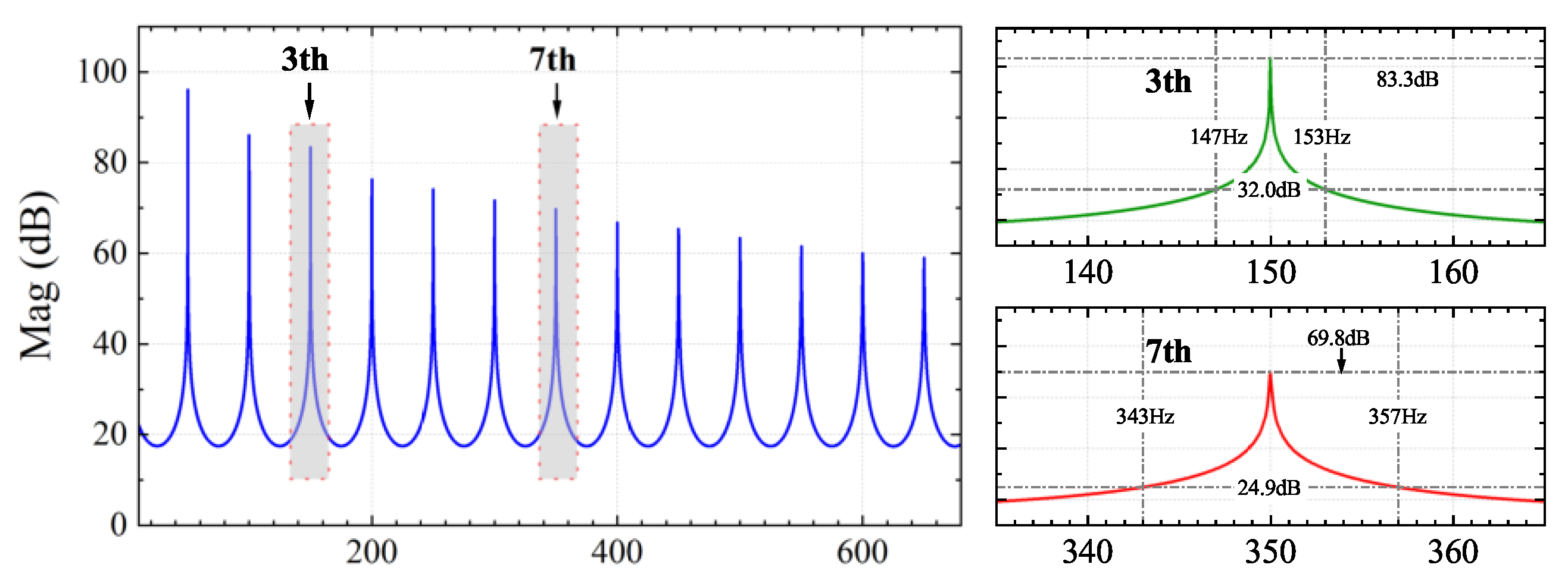
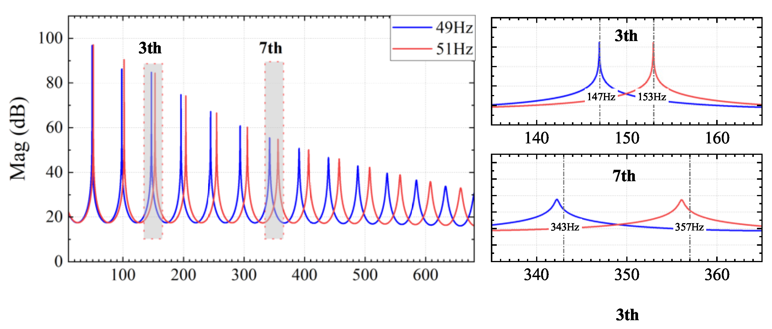
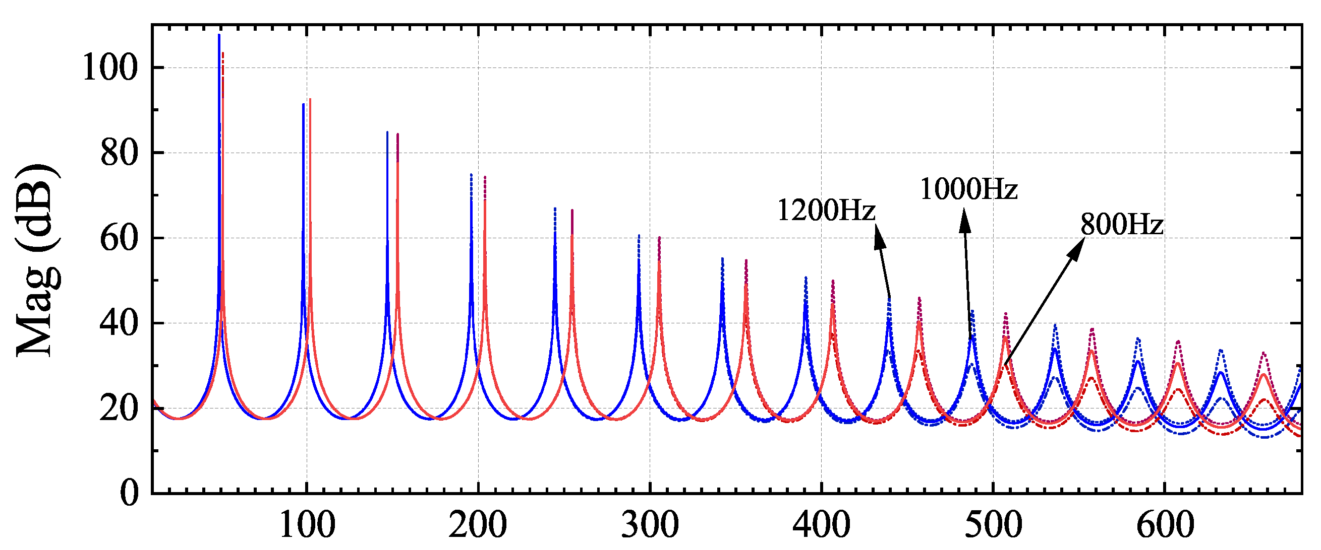
3.3. Harmonic Suppression Analysis

In this subsection, the harmonic suppression capability analysis of the proposed RC is displayed. At the same time, the influence of $Q\left(z_{v1}\right)$ is considered. According to the closed-loop plug-in IMFA-VVS-RC control system, the transfer function from the disturbance $D\left(z_{v1}\right)$ to the tracking error $E\left(z_{v1}\right)$ is obtained. The transfer function represents the ability of the proposed RC to suppress the steady-state errors caused by periodic disturbances. The transfer function is shown in (21):

$$\begin{array}{cc}\hfill \frac{E\left(z_{v1}\right)}{D\left(z_{v1}\right)}& =\frac{-1}{1+[k_{p\_RC}+G_{IMFA-VVS-RC}\left(z_{v1}\right)]P\left(z\right)}\hfill \\ \hfill & =\frac{-1}{1+[k_{p\_RC}+\frac{k_r{z}_{v1}^{-N_v}Q\left(z_{v1}\right)}{1-z_{v1}^{-N_v}Q\left(z_{v1}\right)}S\left(z_{v1}\right)z_{v1}^m]P\left(z\right)}\hfill \\ \hfill & =\frac{-1+z_{v1}^{-N_v}Q\left(z_{v1}\right)}{1-z_{v1}^{-N_v}Q\left(z_{v1}\right)+[k_{p\_RC}(1-z_{v1}^{-N_v}Q\left(z_{v1}\right))+k_r{z}_{v1}^{-N_v}Q\left(z_{v1}\right)S\left(z_{v1}\right)z_{v1}^m]P\left(z\right)}\hfill \\ \hfill \end{array}$$

(21)

When $\omega =2\pi l{f}_r,l=1,2,3\dots$, $z_{v1}^{-N_v}=e^{-j\omega T_{v1}{N}_v}=1$ is satisfied. In this way, (21) can be simplified to (22)

$$\begin{array}{cc}\hfill \frac{E\left(z_{v1}\right)}{D\left(z_{v1}\right)}& =\frac{-1+Q\left(z_{v1}\right)}{1-Q\left(z_{v1}\right)+[k_{p\_RC}(1-Q\left(z_{v1}\right))+k_{r}Q\left(z_{v1}\right)S\left(z_{v1}\right)z_{v1}^m]P\left(z\right)}\hfill \\ \hfill \end{array}$$

(22)

Considering the magnitude, (23) can be obtained.

$$\frac{\left|E\left(z_{v1}\right)\right|}{\left|D\left(z_{v1}\right)\right|}=\frac{\left|1-Q\left(z_{v1}\right)\right|}{\left|1-W\left(z_{v1}\right)\right|}$$

(23)

where $W\left(z_{v1}\right)=Q\left(z_{v1}\right)[1-k_{r}Q\left(z_{v1}\right)S\left(z_{v1}\right)z_{v1}^{m}P\left(z\right)]-k_{p\_RC}\left(z_{v1}\right)(1-Q\left(z_{v1}\right))P\left(z\right)$.

From (23), it can be verified that, when $Q\left(z_{v1}\right)$ is a constant 1, there is no steady-state error. Therefore, although the use of IIR low-pass filter enhances the system stability, it brings about steady-state error. Thus, it is necessary to make $\left|1-W\left(z_{v1}\right)\right|$ as large as possible to reduce the steady-state error when the parameter is designed.

The magnitude response is displayed in Figure 7 for when the VVS scheme is applied in RC. When the frequency changes to 49 Hz and 51 Hz, the resonant frequency of the controller will also change accordingly. As shown in the thumbnail in the upper right corner of Figure 7, when the grid frequency is 49 Hz, the 3rd resonant frequency varies from 150 Hz to 147 Hz. Thus, the 3rd resonant frequency is exactly at the 3rd harmonic frequency. In this way, the proposed RC can still ensure a high gain at the corresponding resonant frequency under the condition of frequency variation. Similarly, this conclusion can also be reached when the grid frequency is 51 Hz. As shown in the thumbnail in the upper left corner of Figure 7, the 7th resonant frequency also varies with the fundamental frequency. Therefore, the proposed RC has good harmonic suppression capability when the frequency varies. However, due to the introduction of a IIR low-pass filter, the 7th resonant frequency is not as accurate as the 3rd resonant frequency, and there is an error within 0.8 Hz.

Figure 8 illustrates the effect of the cutoff frequency of the IIR filter on the resonant frequency and gain of the proposed RC. When the cutoff frequency varies from 800 Hz to 1200 Hz, the gain of the proposed RC becomes higher at the resonant frequencies, which is especially obvious at the high frequencies. At the same time, a higher cutoff frequency can reduce the resonant frequencies shift at high frequencies.

4. Parameter Design

This section shows the design progress of the proposed RC parameter.

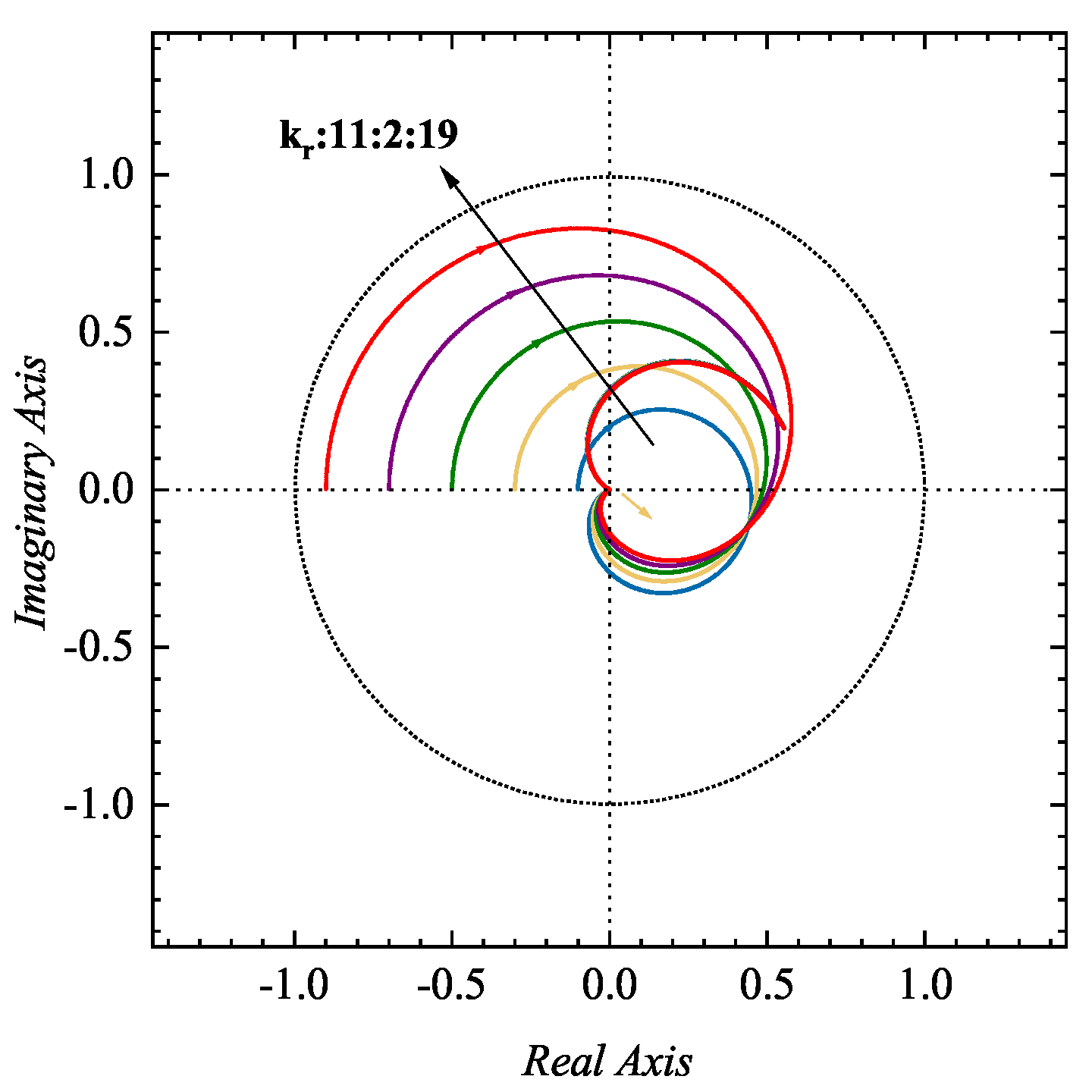
4.1. Design of $k_{p\_RC}$

As shown in Figure 9, the changing progress of the pole locations when $k_{p\_RC}$ increases from 6 to 14 is shown. In the range $k_{p\_RC}=6$ to $k_{p\_RC}=14$, the poles of $G_p\left(z\right)$ are all in the unit circle, and the system remains stable. As $k_{p\_RC}$ increases, poles on the real axis approach the origin, while poles not on the real axis approach the unit circle. To guarantee the system stability, $k_{p\_RC}$ is chosen as 10.

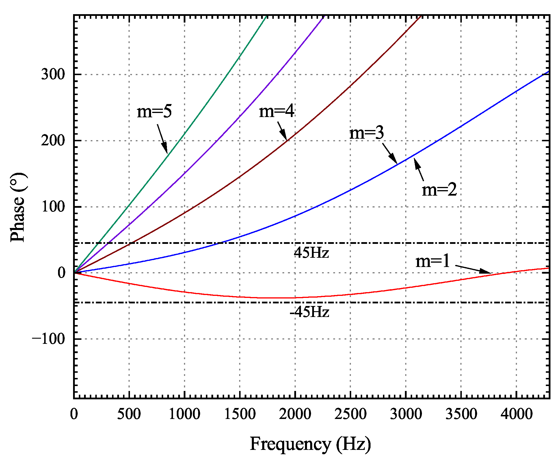
4.2. Design of m

The phase lead compensation filter $z_{v1}^m$ needs to compensate for the phase lag of $G_p\left(z\right)$ to 0°. The phase response of $G_p\left(z\right)z_{v1}^m$ when m changes from 1 to 5 is shown in Figure 10. When $m=1$, the phase response of $G_p\left(z\right)z_{v1}^m$ can be kept in the range of −45° to 45° until 4000 Hz. In this way, the best choice for m is 1.

4.3. Design of $k_r$

As shown in Figure 11, the Nyquist curves of the $T\left(z\right)$ approach the unit circle as $k_r$ increases from 11 to 19. The values of $k_r$ of adjacent curves differ by 2. To ensure the system stability, $k_r$ should be as small as possible. But correspondingly, a small $k_r$ causes a slow convergence rate. According to the trade-off of the stability margin and the convergence rate, we select $k_r$ to be 15.

4.4. Design of Cutoff Frequency

Considering the complexity of the design, the second-order Butterworth low-pass filter is selected. According to the influence of cutoff frequency on system stability and harmonic suppression capability mentioned above, the cutoff frequency is selected as 1200 Hz.

$$Q\left(z_{v1}\right)=\frac{0.0913+0.1826z_{v1}^{-1}+0.0913z_{v1}^{-2}}{1-0.9824z_{v1}^{-1}+0.3476z_{v1}^{-2}}$$

(24)

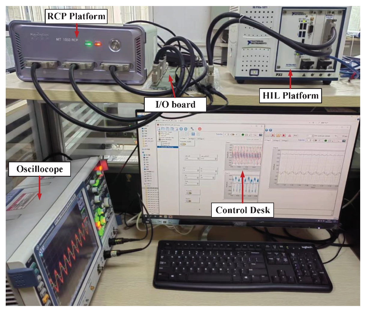
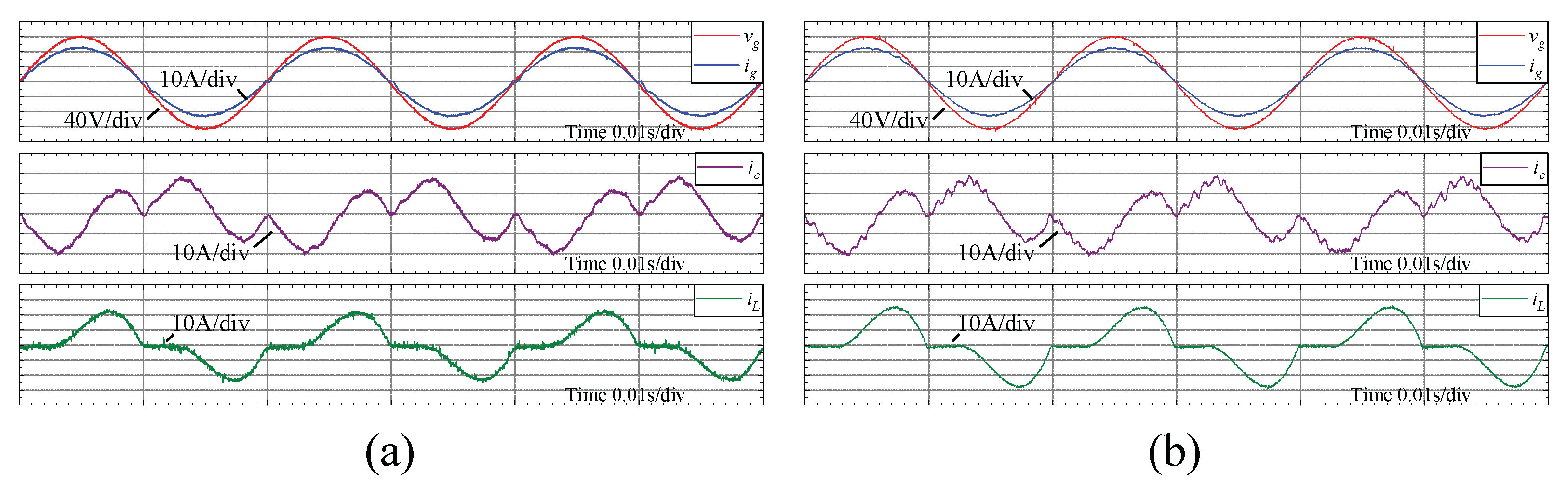
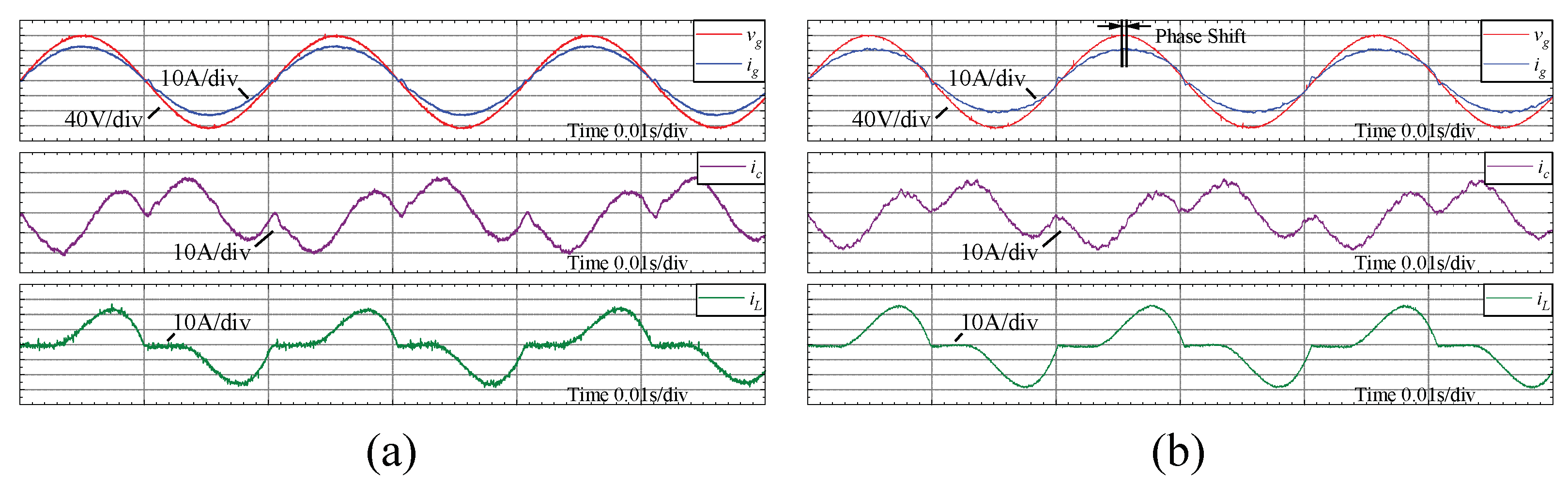
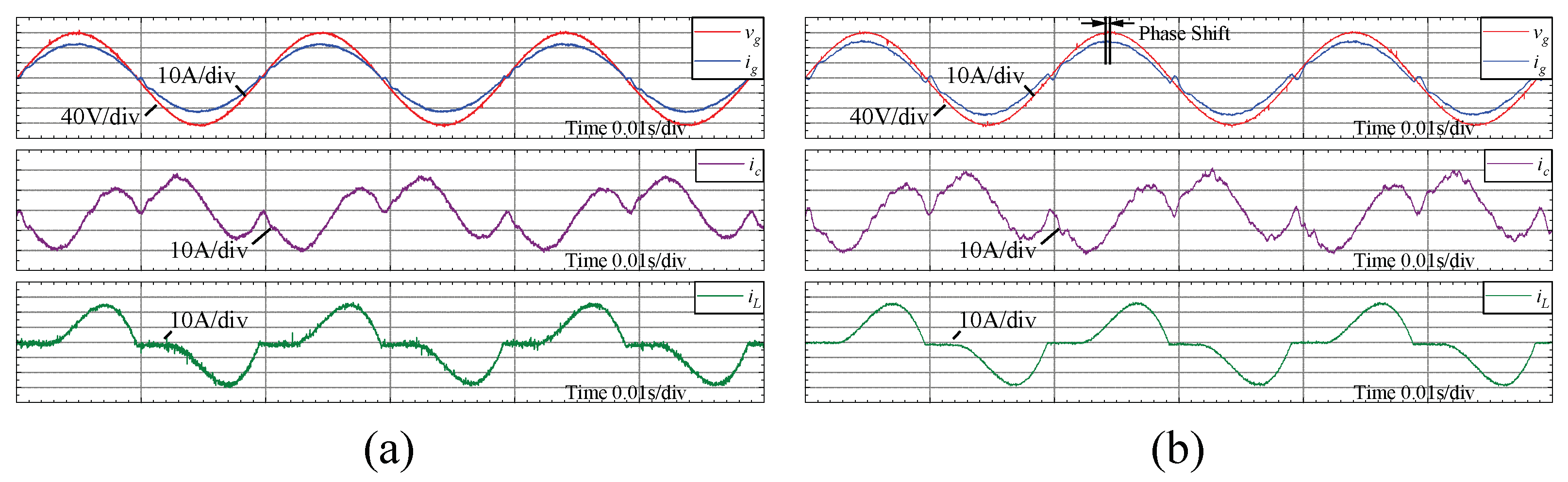
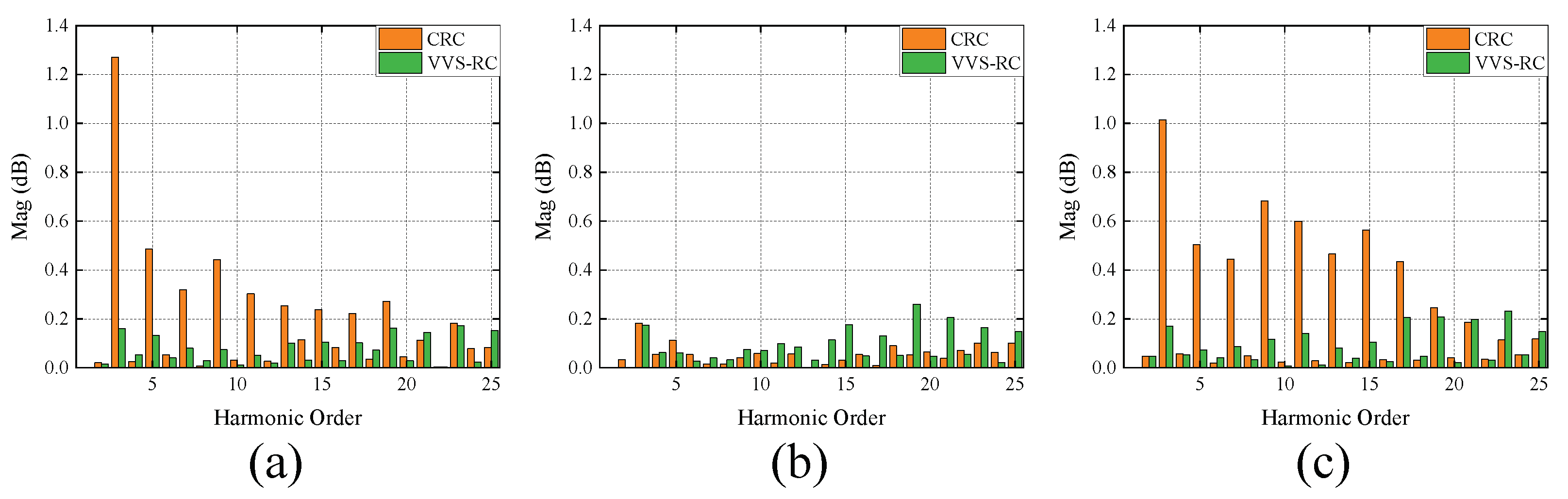
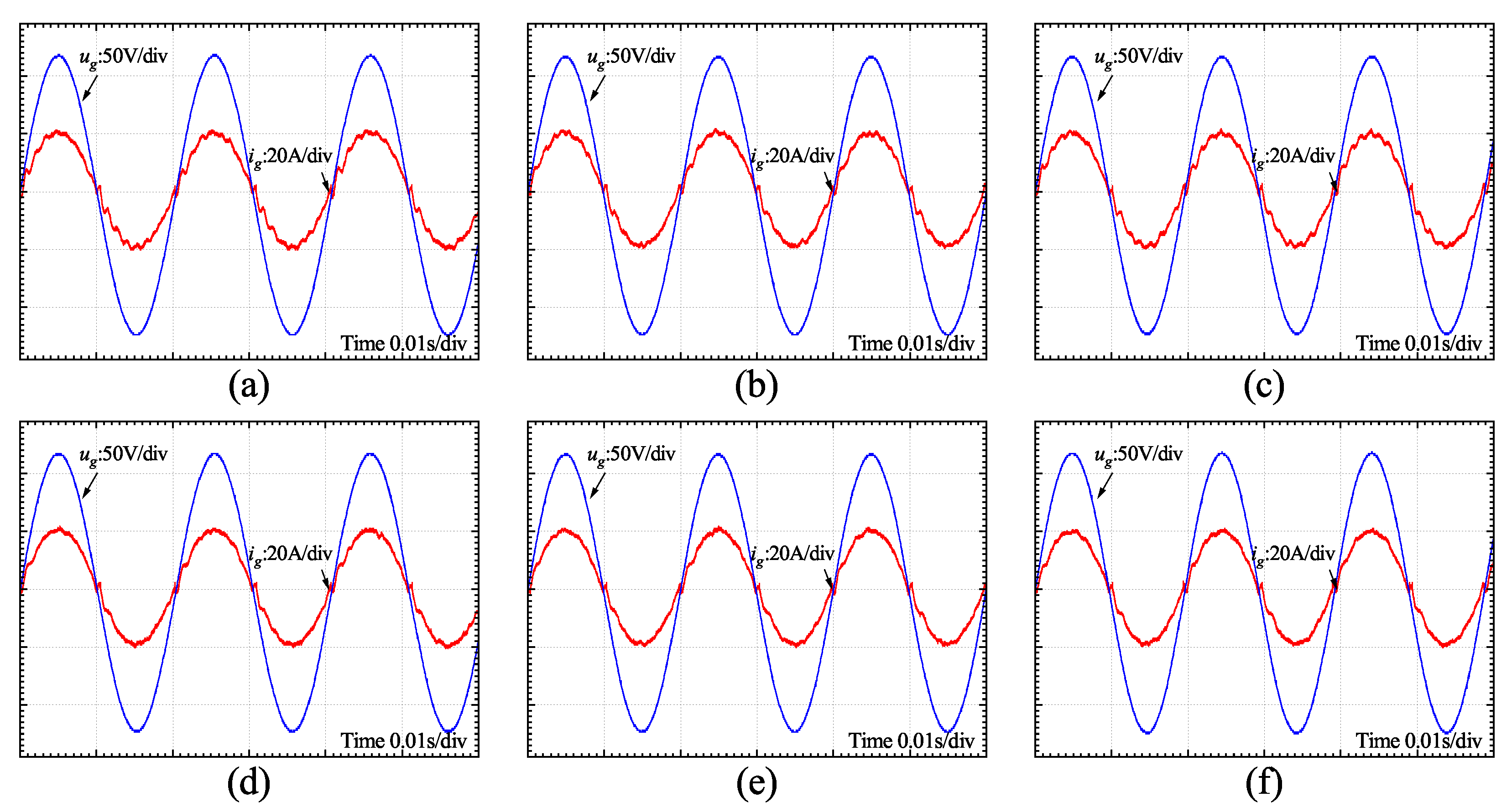
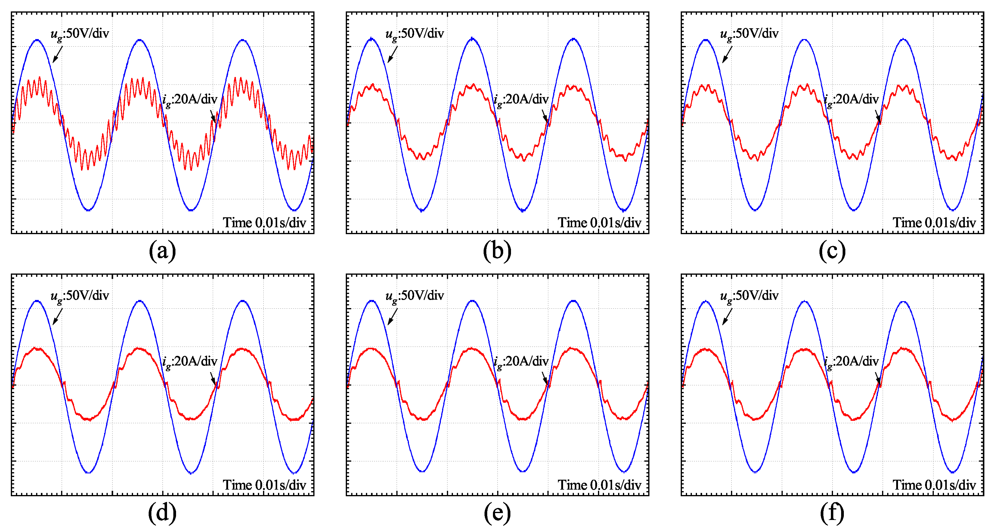
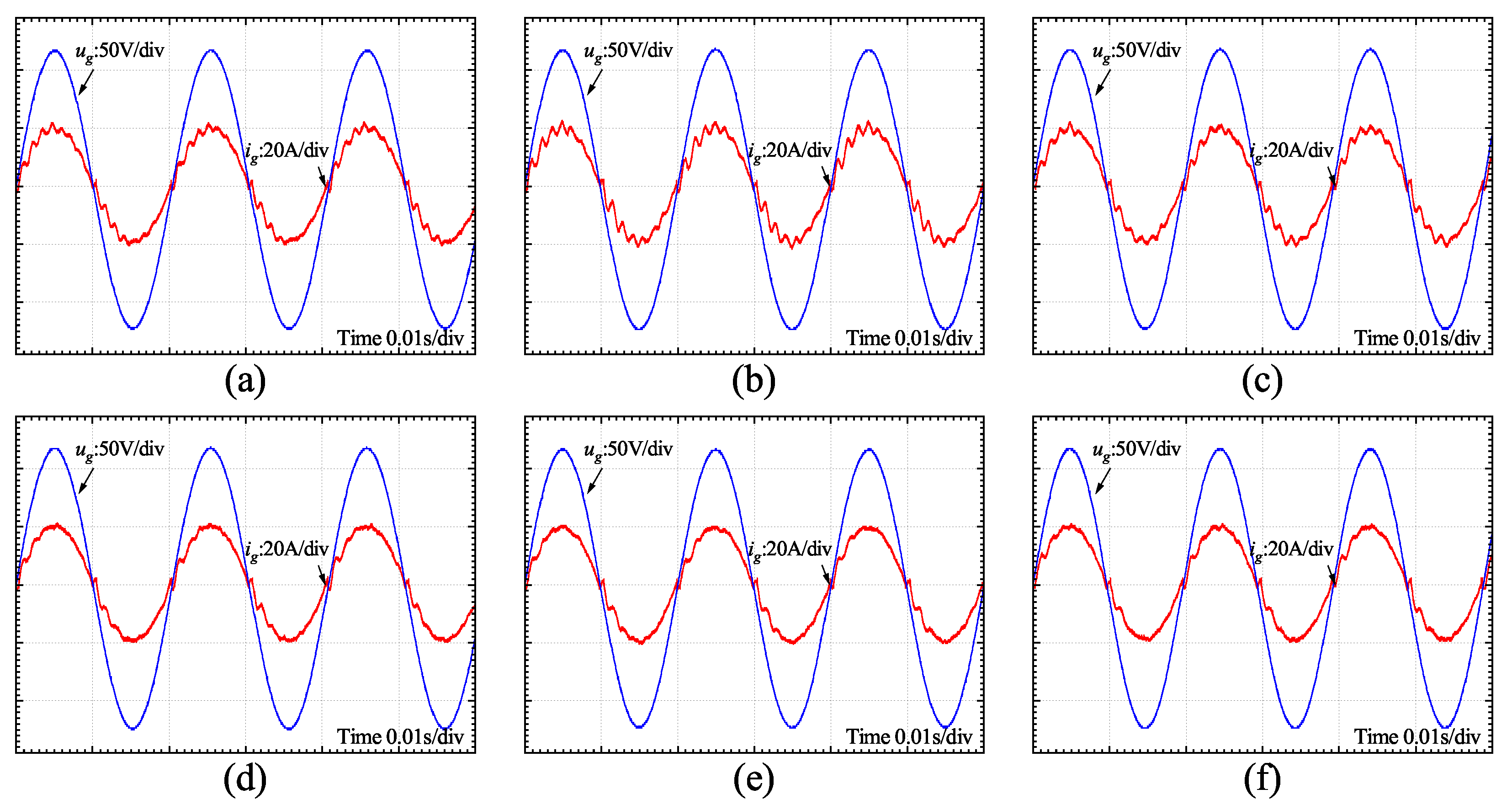
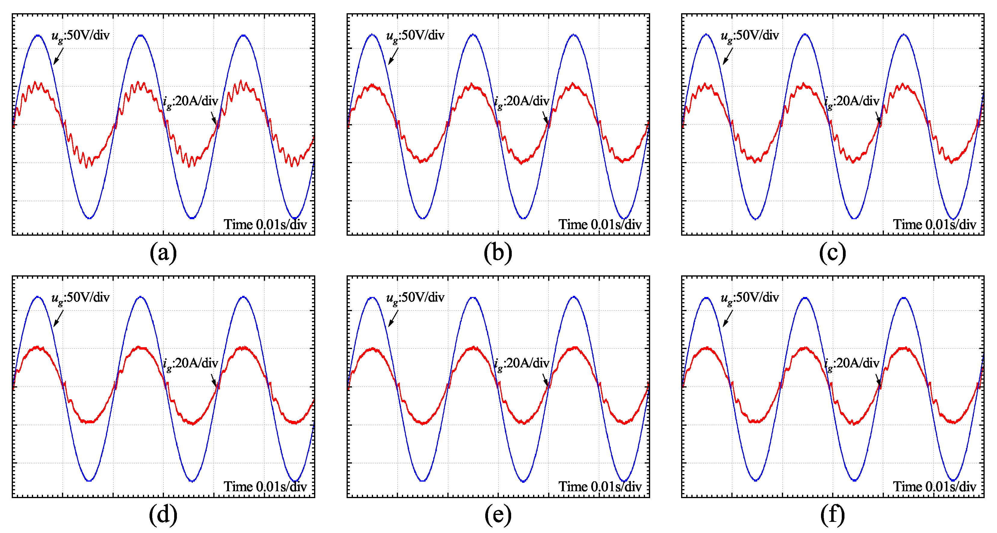
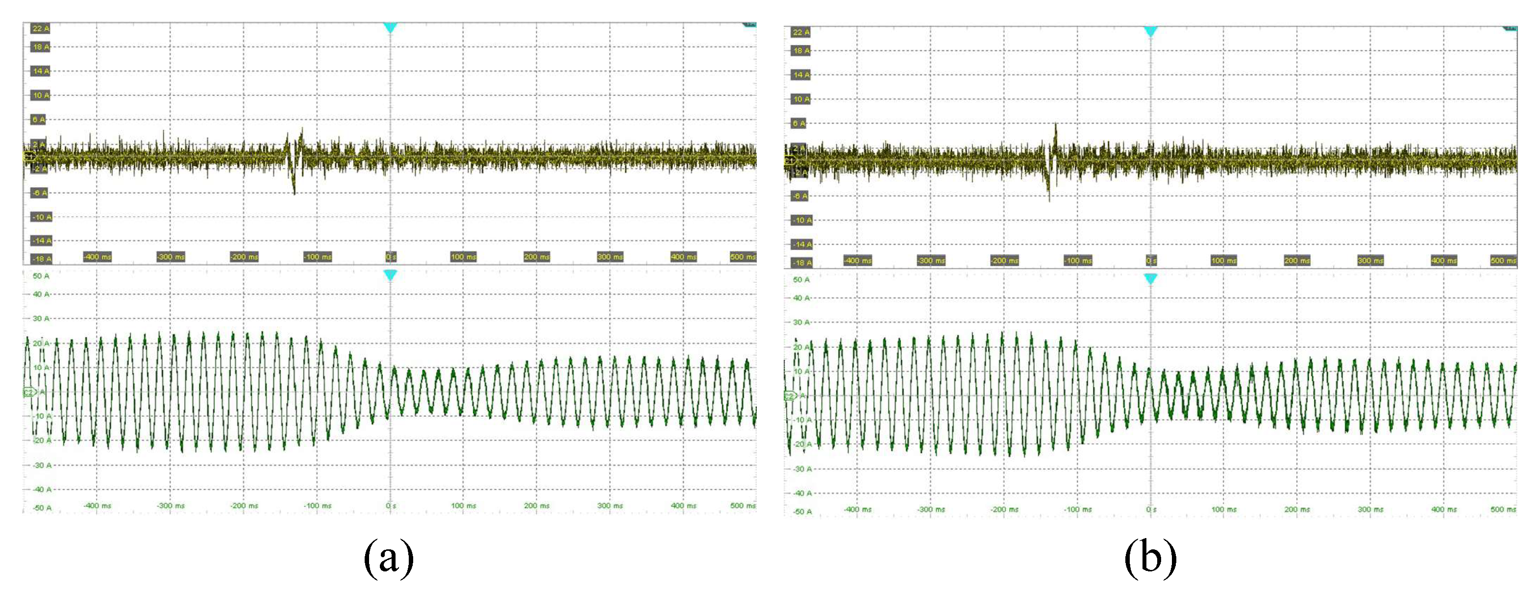
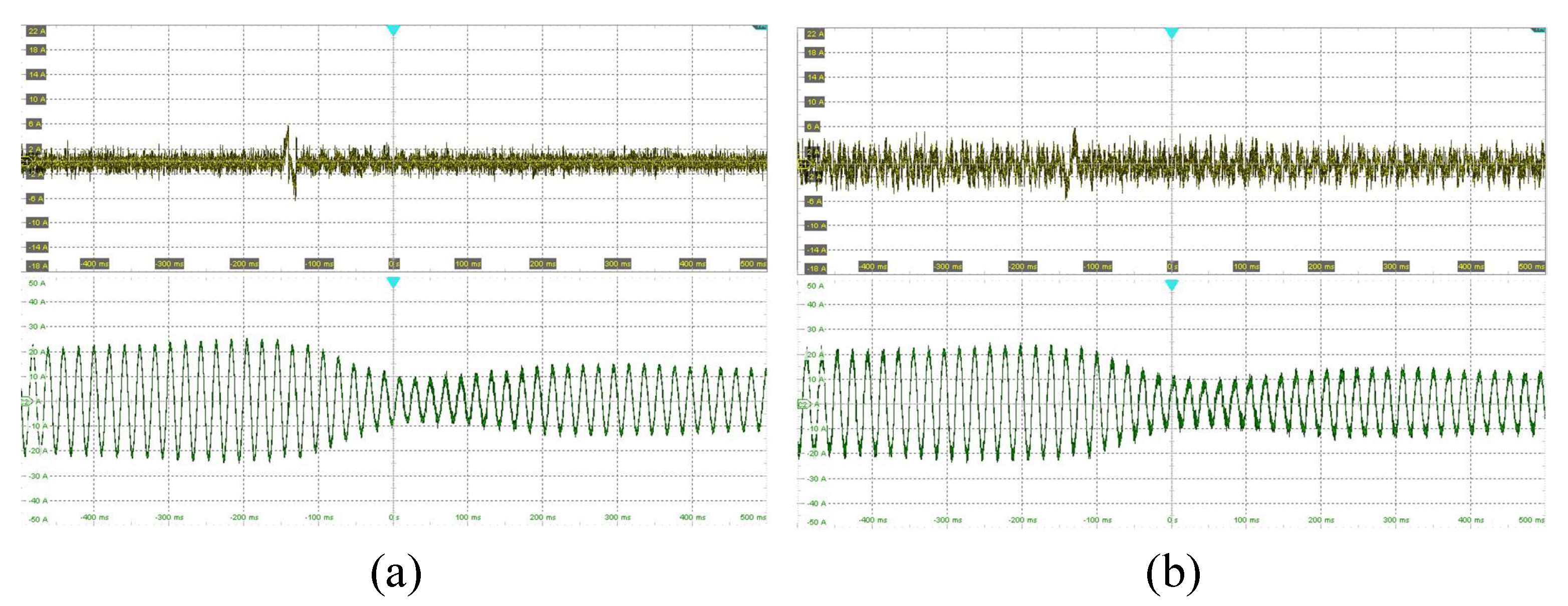
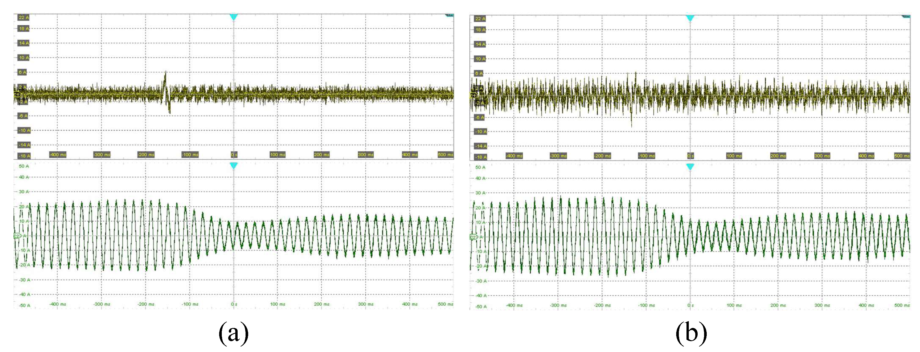
5. Experiment

Before building the experimental platform, the main circuit and control loop need to be modeled mathematically. The control loop and main circuit of the single-phase APF system are displayed in Figure 12. The main circuit is composed of a power grid, nonlinear load, LCL filter, and H-bridge. $u_g$ is the grid voltage, $i_g$ is the grid current, and $L_g$ is the grid inductor. The nonlinear loads consist of an uncontrolled bridge rectifier, an inductor $L_r$, a capacitor $C_r$, and a resistor R. $i_L$ is the current of the nonlinear load. The LCL filter consists of $L_1$, $L_2$, and $C_f$. $i_1$ and $i_2$ are the current of $L_1$ and $L_2$, respectively. $R_d$ is passive damping. $u_{inv}$ is the output voltage of the inverter. C is the capacitor in the DC side of the inverter. $u_{dc}$ is the DC bus voltage.

Because the current flowing through the capacitor $C_f$ is small, the capacitor branch can be ignored in the mathematical modeling process. Therefore, the LCL filter can be approximately regarded as an L filter. The grid inductance $L_g$ and grid-side inductance $L_1$ of LCL filter are considered simultaneously. Define the equivalent grid-side inductance $L_{1e}=L_1+L_g$. Let $L=L_{1e}+L_2$ and $i_c=i_1=i_2$. (25) and Equation (26) can be obtained by Kirchhoff’s law. According to (25) and (26), the model of the single-phase shunt APF system can be established.

$$\left\{\begin{array}{c}L\frac{d{i}_c}{dt}=u_{inv}-u_g\\ \\ \\ C\frac{d{u}_{dc}}{dt}=S\left(t\right)i_c\end{array}\right.$$

(25)

$$S\left(t\right)=\left\{\begin{array}{cc}1& G1,G4on\\ -1& G2,G3on\end{array}\right.$$

(26)

In order to ensure that the total energy of the APF converter remains constant, $u_{dc}^2$ should be kept constant during the control process. As shown in Figure 12, the PI controller is selected as the outer loop control strategy. To obtain the reference grid current $i_{gref}$ synchronized with the grid voltage, the output of the PI controller is multiplied by the phase of the grid voltage. In summary, (27) and (28) can be obtained. The proposed RC is selected as the inner loop control strategy to control the grid current.

$$u=k_p(u_{{}_{dcref}}^2-u_{dc}^2)+k_i\int (u_{{}_{dcref}}^2-u_{dc}^2)dt$$

(27)

$$i_{gref}=u·u_g$$

(28)

According to the parameters shown in the

Table 1. APF simulation model parameters.

Parameters	Symbol	Values
Nonlinear load inductor	$L_r$	4 mH
Nonlinear load capacitor	$C_r$	4400 $\mathsf{\mu }$F
Nonlinear load resistance	R	8 $\mathsf{\Omega }$
Grid Voltage	$u_g$	$120/\sqrt{2}$ V
Equivalent grid-side inductance	$L_{1e}$	0.1 mH
Inverter-side inductance	$L_2$	3.5 mH
Filter capacitor	$C_f$	7 $\mathsf{\mu }$F
Passive damping	$R_d$	10 $\mathsf{\Omega }$
Sampling frequency	$f_s$	10 kHz
Grid frequency	$f_0$	50 Hz
DC bus capacitor	C	2200 $\mathsf{\mu }$F
DC bus voltage	$u_{dcref}$	250 V

, a single-phase shunt APF system model based on NI PXIe-1071 and YuanKuan MT1050 is established. The setups are shown in the Figure 13. We select $k_p=1.5$, $k_i=30$, $k_{p\_RC}=10$, $k_r=15$, $Q\left(z_{v1}\right)=0.1z_{v1}+0.8+0.1z_{v1}^{-1}$, $m=1$, $S\left(z\right)=1$, and $N_v=120$. The LCL single-phase APF model was configured in the StarSim Hardware-in-the-Loop (HIL) platform with a time step of 1 $\mathsf{\mu }$s. The controller was configured in the FPGA-based StarSim rapid control prototyping (RCP) platform with a time step of 100 $\mathsf{\mu }$s.

As shown in Figure 14, CRC and the proposed RC can reduce the harmonics injected into the grid. It can be proven that with CRC, the THD of the grid current $i_g$ is 2.02%. Meanwhile, with the proposed RC, the THD of grid current $i_g$ is 2.81%. By comparing Figure 14a,b, it can be proven that CRC and the proposed RC have similar control effects under the condition of 50 Hz. As shown in Figure 14, with CRC and the proposed RC, the phase of the grid current is synchronized with the grid voltage. In this way, the unit power factor is maintained.

The output current waveform at 51 Hz is shown in Figure 15. The THD of the grid current $i_g$ is 7.72% when CRC is adopted, and the THD of the grid current $i_g$ is 2.84% when the proposed RC is adopted. In the same way, Figure 16 shows the output current waveform at 49 Hz. When CRC is adopted, the THD of the grid current $i_g$ is 7.53%. Furthermore, the THD of the grid current $i_g$ is 2.43% when the proposed RC is adopted. It can be verified that the harmonic suppression ability of the proposed is better than that of CRC when the frequency varies. As can be seen from Figure 15b and Figure 16b, CRC works at an abnormal frequency, resulting in a phase shift between the grid voltage $u_g$ and grid current $i_g$.

In Figure 17, the FFT analysis of the grid current is displayed. Figure 17 compares the magnitude from the second harmonic to the 25th harmonic when the proposed RC (the green columns) and the CRC (the orange columns) are used. As shown in Figure 17b, when the grid frequency is normal (50 Hz), the harmonic magnitudes of the proposed RC and CRC are relatively close, which is the same as the conclusion drawn in Figure 14 above. As shown in Figure 17a,c, when the proposed RC is used, the harmonic magnitude of $i_g$ is smaller at low and middle frequencies to those of the CRC. Therefore, it is proven from another angle that the proposed RC still has a good harmonic suppression capability when the frequency varies.

When the grid frequency is between 49 Hz and 51 Hz, multiple experiments are repeated and the THD of the grid current $i_g$ and load current $iL$ is calculated. The results obtained are displayed in

Table 2. The THD of the grid current $i_g$.

	49 Hz	49.5 Hz
CRC	7.53%	4.73%
IMFA-VVS-RC	2.43%	2.51%
	50 Hz
CRC	2.02%
IMFA-VVS-RC	2.81%
	50.5 Hz	51 Hz
CRC	4.51%	7.72%
IMFA-VVS-RC	2.50%	2.84%

and

Table 3. The THD of the load current $i_L$.

49 Hz	49.5 Hz	50 Hz	50.5 Hz	51 Hz
41.05%	40.8%	40.62%	40.41%	40.2%

. The THD of the load current is around 41%. Compared Table 2 with Table 3, the harmonic suppression function of APF is shown. With the increase in frequency variation, the THD gained with the use of the proposed RC always remains below 5%, in line with the IEEE std 1547. On the contrary, when the CRC is used, the THD of $i_g$ increases gradually when the variation increases. Compared with CRC, the proposed RC can operate over a wider range of grid frequencies.

In order to verify the parameter robustness of the two controllers, the grid-side inductance $L_{1e}$, the Inverter-side inductance $L_{1e}$, and filter capacitor $C_f$ are changed. The waveforms of $u_g$ and $i_g$ are shown in Figure 18, and the parameters of LCL filter are shown in Table 1. In this case, the quality of the current controlled by RC with FIR filter and IIR filter is similar. At the same time, due to the implementation of VVS technology, the RC control effect is not affected by frequency variation. Figure 19, Figure 20 and Figure 21 respectively show the waveforms of $i_g$ and $u_g$ when $L_{1e}$, $L_2$, and $C_f$ are changed. Comparing the above figures with Figure 18, when an IIR filter is adopted, the control effect of the $i_g$ changes slightly when LCL parameters vary. Compared with the IIR filter, the parameter robustness of the FIR filter is worse, and the quality of the grid current deteriorates with the parameter variation of the LCL filter.

When the load changes from 16 $\mathsf{\Omega }$ to 8 $\mathsf{\Omega }$, the steady-state error of the grid current at 50 Hz is shown in Figure 22a,b. When CRC is used, the steady-state error can reach stability after 16 periods. At the same time, when the proposed RC is used, the steady-state error can reach stability within 16 periods. Comparing Figure 22a,b, it is proven that the response speed of the proposed RC is close to that of CRC. When the grid frequency is 49 Hz or 51 Hz, the steady-state error of the grid current is shown in Figure 23a,b and Figure 24a,b. As shown in Figure 23b and Figure 24b, the error is larger than that of Figure 23a and Figure 24a.

6. Conclusions

This paper proposes the use of a repetitive controller based on VVS. In order to improve the robustness of the system, a IIR low-pass filter $Q\left(z\right)$ is added to the proposed RC. The VVS scheme realizes a variable sampling frequency by using a virtual sampling unit. In this way, RC can still achieve a better control effect under the condition of frequency variation. The experimental results show that compared with CRC, the harmonic suppression capability of the proposed RC is stronger when RC is 49 Hz and 51 Hz. When the frequency is 49 Hz, the THD of the grid current is 7.72% when CRC is used and 2.84% when the proposed RC is used. When the frequency is 51Hz, the THD of the grid current is 7.53% when CRC is used and 2.43% when the proposed RC is used. Compared with CRC, the proposed RC still has good harmonic suppression capability in the case of frequency variation. Moreover, the harmonic suppression capability of the proposed RC is similar to that of CRC at 50 Hz. When the frequency is 50 Hz, the THD of the grid current is 2.02% when CRC is used and 2.81% when the proposed RC is used. The proposed RC does not affect the harmonic suppression process under normal working conditions. In addition, the harmonic suppression capability of the proposed RC is still excellent when the grid-side inductance value changes. When $L_{1e}$ changes from 0.1 mH to 2.6 mH, the system is no longer stable when CRC is used. When the proposed RC is used, the system remains stable. When $L_2$ and $C_f$ vary, the grid current waveform will deteriorate when CRC is used. Therefore, it can be proved that the parameter robustness of the proposed RC is better than that of CRC. When the grid frequency is 50 Hz, the grid current has a similar dynamic response when the proposed RC and CRC are used. When the grid frequency varies, the grid current has a smaller steady-state error when the proposed RC is used.

References

- Mishra, A.K.; Das, S.R.; Ray, P.K.; Mallick, R.K.; Mohanty, A.; Mishra, D.K. PSO-GWO optimized fractional order PID based hybrid shunt active power filter for power quality improvements. IEEE Access 2020, 8, 74497–74512. [Google Scholar] [CrossRef]
- Chen, D.; Xiao, L.; Yan, W.; Li, Y.; Guo, Y. A heat dissipation design strategy based on computational fluid dynamics analysis method for shunt active power filter. Energy Rep. 2022, 10, 229–238. [Google Scholar] [CrossRef]
- Fang, J.; Xiao, G.; Yang, X.; Tang, Y. Parameter design of a novel series-parallel-resonant LCL filter for single-phase half-bridge active power filters. IEEE Trans. Power Electron. 2017, 32, 200–217. [Google Scholar] [CrossRef]
- Franca, B.W.; Aredes, M.; da Silva, L.F.; Gontijo, G.F.; Tricarico, T.C.; Posada, J. An Enhanced Shunt Active Filter Based on Synchronverter Concept. IEEE J. Emerg. Sel. Top. Power Electron. 2022, 10, 494–505. [Google Scholar] [CrossRef]
- Echalih, S.; Abouloifa, A.; Lachkar, I.; Hekss, Z.; El Aroudi, A.; Giri, F.; Al-Numay, M.S. Nonlinear Control Design and Stability Analysis of Single Phase Half Bridge Interleaved Buck Shunt Active Power Filter. IEEE Trans. Circuits Syst. I-Regul. Pap. 2022, 69, 2117–2128. [Google Scholar] [CrossRef]
- Kumar, R.; Bansal, H.O.; Gautam, A.R.; Mahela, O.P.; Khan, B. Experimental Investigations on Particle Swarm Optimization Based Control Algorithm for Shunt Active Power Filter to Enhance Electric Power Quality. IEEE Access 2022, 10, 54878–54890. [Google Scholar] [CrossRef]
- Frifita, K.; Boussak, M. A novel strategy for high performance fault tolerant control of shunt active power filter. IEEE Electr. Eng. 2022, 104, 2531–2541. [Google Scholar] [CrossRef]
- De souza, L.L.; Rocha, N.; Fernandes, D.A.; De Sousa, R.P.R.; Jacobina, C.B. Grid Harmonic Current Correction Based on Parallel Three-Phase Shunt Active Power Filter. IEEE Trans. Power Electron. 2022, 37, 1422–1434. [Google Scholar]
- De Roover, D.; Bosgra, O.H.; Steinbuch, M. Internal-model-based design of repetitive and iterative learning controllers for linear multivariable systems. Int. J. Control 2000, 73, 914–929. [Google Scholar] [CrossRef]
- Chen, D.; Chen, H.; Hu, Y.; Chen, G. A novel serial structure repetitive control strategy for shunt active power filter. Compel-Int. J. Comp. Math. Electr. Electron. Eng. 2019, 38, 199–215. [Google Scholar] [CrossRef]
- Pandove, G.; Singh, M. Robust Repetitive Control Design for a Three-Phase Four Wire Shunt Active Power Filter. IEEE Trans. Ind. Inform. 2019, 15, 2810–2818. [Google Scholar] [CrossRef]
- Neto, R.C.; Neves, F.A.S.; de Souza, H.E.P. Complex nk + m repetitive controller applied to space vectors: Advantages and stability analysis. IEEE Trans. Power Electron. 2021, 9, 3573–3590. [Google Scholar] [CrossRef]
- Geng, H.; Zheng, Z.; Zou, T.; Chu, B.; Chandra, A. Fast Repetitive Control with Harmonic Correction Loops for Shunt Active Power Filter Applied in Weak Grid. IEEE Trans. Ind. Appl. 2019, 55, 3198–3206. [Google Scholar] [CrossRef]
- Chen, Z.; Zha, H.; Peng, K.; Yang, J.; Yan, J. A design method of optimal PID-based repetitive control systems. IEEE Access 2020, 8, 139625–139633. [Google Scholar] [CrossRef]
- Pan, G.; Gong, F.; Jin, L.; Wu, H.; Chen, S. LCL APF based on fractional-order fast repetitive control strategy. J. Power Electron. 2021, 21, 1508–1519. [Google Scholar] [CrossRef]
- Jian, L.; Li, X.; Zhu, J.; Hao, Z.; Li, F. Dual closed-loops current controller for a 4-leg shunt APF based on repetitive control. Int. J. Electron. 2019, 106, 349–364. [Google Scholar] [CrossRef]
- Escobar, G.; Hernandez-Gomez, M.; Valdez-Fernandez, A.A.; Lopez-Sanchez, M.J.; Catzin-Contreras, G.A. Implementation of a 6n ± 1 repetitive controller subject to fractional delays. IEEE Trans. Ind. Electron. 2015, 62, 444–452. [Google Scholar] [CrossRef]
- Yang, Y.; Zhou, K.; Blaabjerg, F. Enhancing the frequency adaptability of periodic current controllers with a fixed sampling rate for grid-connected power converters. IEEE Trans. Power Electron. 2016, 31, 7273–7285. [Google Scholar] [CrossRef]
- Zhao, Q.; Ye, Y. Fractional phase lead compensation RC for an inverter: Analysis, design, and verification. IEEE Trans. Ind. Electron. 2017, 64, 3127–3136. [Google Scholar] [CrossRef]
- Liu, Z.; Zhang, B.; Zhou, K. Universal fractional-order design of linear phase lead compensation multirate repetitive control for PWM inverters. IEEE Trans. Ind. Electron. 2017, 64, 7132–7140. [Google Scholar] [CrossRef]
- Zhao, Q.; Chen, S.; Wen, S.; Qu, B.; Ye, Y. A frequency adaptive PIMR-type repetitive control for a grid-tied inverter. IEEE Access 2018, 6, 65418–65428. [Google Scholar] [CrossRef]
- Zhu, M.; Ye, Y.; Xiong, Y.; Zhao, Q. Parameter robustness improvement for repetitive control in grid-tied inverters using an IIR filter. IEEE Trans. Power Electron. 2021, 36, 8454–8463. [Google Scholar] [CrossRef]
- Liu, T.; Wang, D.; Zhou, K. High-performance grid simulator using parallel structure fractional repetitive control. IEEE Trans. Power Electron. 2016, 31, 2669–2679. [Google Scholar] [CrossRef]
- Liu, T.; Wang, D. Parallel structure fractional repetitive control for PWM inverters. IEEE Trans. Ind. Electron. 2015, 62, 5045–5054. [Google Scholar] [CrossRef]
- Kolluri, S.; Gorla, N.B.Y.; Panda, S.K. Capacitor voltage ripple suppression in a modular multilevel converter using frequency-adaptive spatial repetitive-based circulating current controller. IEEE Trans. Power Electron. 2020, 35, 9839–9849. [Google Scholar] [CrossRef]
- Huo, X.; Wang, M.; Liu, K.-Z.; Tong, X. Attenuation of position-dependent periodic disturbance for rotary machines by improved spatial repetitive control with frequency alignment. IEEE-ASME Trans. Mechatron. 2020, 25, 339–348. [Google Scholar] [CrossRef]
- Kolluri, S.; Gorla, N.B.Y.; Sapkota, R.; Panda, S.K. A new control architecture with spatial comb filter and spatial repetitive controller for circulating current harmonics elimination in a droop-regulated modular multilevel converter for wind farm application. IEEE Trans. Power Electron. 2019, 34, 10509–10523. [Google Scholar] [CrossRef]
- Liu, Z.; Zhang, B.; Zhou, K.; Wang, J. Virtual variable sampling discrete fourier transform based selective odd-order harmonic repetitive control of DC/AC converters. IEEE Trans. Power Electron. 2018, 33, 6444–6452. [Google Scholar] [CrossRef]
- Liu, Z.; Zhou, K.; Yang, Y.; Wang, J.; Zhang, B. Frequency-adaptive virtual variable sampling-based selective harmonic repetitive control of power inverters. IEEE Trans. Ind. Electron. 2021, 68, 11339–11347. [Google Scholar] [CrossRef]
- Zhao, Q.; Ye, Y. A PIMR-Type Repetitive Control for a Grid-Tied Inverter: Structure, Analysis, and Design. IEEE Trans. Power Electron. 2018, 33, 2730–2739. [Google Scholar] [CrossRef]