Simplified Numerical Model for Transient Flow of Slurries at Low Concentration

Abstract

Rapid transients are particularly dangerous in industrial hydro-transport systems, where solid-liquid mixtures are transported via long pressure pipelines. A mathematical description of such flow is difficult due to the complexity of phenomena and difficulties in determining parameters. The main aim of the study was to examine the influence of the simplified mixture density and wave celerity description on satisfactory reproduction of pressure characteristics during the transient flow of slurry at low concentrations. The paper reports and discusses the selected aspects of experimental and numerical analyses of transient slurry flow in a polyethylene pipe. The experiments were conducted by using the physical model of a slurry’s transportation pressure. The aim of the experiments was to determine the wave celerity during a transient flow in slurries. A low concertation of slurries, which was used during experiments, is typical for one of the biggest slurry networks in Poland. A comparison of the effects of different wave celerity descriptions was performed. The research reported that the theoretical formulas for slurry wave celerity and mixture density were not sufficiently accurate to obtain satisfactory compliance between calculations and observations. To improve the model, the experimental values of wave celerity and the concept of equivalent mixture density have been applied to indirectly consider the influence of variable mixture parameters. With such modifications, the calculated pressure characteristics in all analyzed episodes demonstrated satisfactory compliance with observations. The simplified approach proved to be effective in properly reproducing the intensity and frequency of rapid pressure changes.

1. Introduction

Pipe flows of solid–liquid mixtures in the form of slurries are an important alternative to the conventional method of solid particle transportation. Hydro-transport is particularly effective in mining, chemical, petroleum or nuclear industries, where solid material is conveyed from remote locations, often not accessible by traditional means of transport, via long industrial pipelines [1,2,3,4,5] to target installations or storage locations. Transportation of solid materials through pipelines with the use of water as a carrier liquid is also present in civil and environmental engineering, e.g., in waste, drainage or biomass systems. In some cases, transporting the mixture instead of a pure liquid is a side effect of industrial processes, not an intended method of transporting solid particles.

The dynamics of the slurry flow in each case were strongly dependent on the interrelationship of many different factors, among which the most important are the features of the mixture (both liquid and solid phases), the parameters of the hydraulic transportation system, and the flow velocity. The essential characteristics significantly affecting the flow behavior are: solid phase concentration, particle size, weight and shape distribution, liquid viscosity, critical deposition velocity, level of turbulence, flow velocity distribution within the cross-section area, and size, shape and elevation variability of the conduit and the scale of the phenomenon (natural or laboratory installation). Depending on the relationship among the above-mentioned parameters, different phenomena may be observed during the slurry flow.

If the solid particles are sufficiently small and light [1,6], the inertial effects have a poor influence on the particle dynamics. The solids have no or only a slight tendency to settle out, and thus, they are well distributed across the cross-section area, and the bulk slurry velocity is not affected by inertial effects. As a consequence, in such cases, for computational and design purposes, the mixture may be treated as a pseudo-homogeneous medium. The same model may be applied if the particles tend to settle on the bottom due to their size, but the flow is turbulent enough to keep the solid concentration approximately uniform and the velocity distribution axisymmetric within the pipe cross-section. Finally, the third type of slurry that may be classified as non-settling and pseudo-homogeneous is a special type of multi-sized mixture (usually clay water slurry plus larger particles) in which the viscosity becomes high enough to cause the larger particles to settle very slowly. In all three cases, the mixture may be considered as a single-phase pseudo-fluid, with specific bulk parameters ‘averaged’ for the slurry, or as a two-phase mixture (with separated parameters of both phases) but with a uniform solid concentration in the cross-section and axisymmetric velocity distribution, usually represented by one averaged value.

In various practical cases, however, solid particles are larger, and thus the inertial effects affect their dynamics. The velocity of solid particles is different from the liquid velocity, and the particles are not uniformly distributed across the pipeline cross-section. Thus, both phases should be treated separately. As a consequence, the mixture is a two-phase medium and should be treated as heterogeneous [6]. Additionally, in many cases, the solid material is intensely polydisperse, with a range of particle sizes that may span three orders of magnitude [5,7]. In such a case, solids of different sizes demonstrate different flow velocities, which makes the slurry dynamics more complex (modified velocity and concentration distributions). The smaller particles are carried by the liquid, while the larger settle out and create a deposit. The presence of the bottom layer obviously influences flow behavior (modulates flow area, shear stress, velocity fields and particle flux) and makes the dynamics of the slurry even more complex [8,9]. In extreme cases, the mixture is so heterogeneous that it should be treated as multi-phased [10].

In most cases, for slurry flow investigations, a steady flow model is applied. It is commonly used to describe the hydraulic conditions in the pipeline for the purposes of pipeline design and operation or slurry pump selection [1,3,5,6,7,9]. Most efforts were focused on predicting the pressure drop, concentration profile, velocity distribution and deposition velocity in slurry flow. Less research is concentrated on liquid-solid interactions, particle velocity fluctuations, bed formation, morphology and dynamics, plug formation and transitional flow regime identification (e.g., [3]).

In the case of a transient flow of a slurry in a pressure system, the description of the problem becomes more complex, especially when compared with liquid flows. Several current publications on various issues of transient flows may be found, for example, repair systems for flexible conduits [11], liquids other than water [12] or the problem of cavitation [13]. The area of transient flows in the sludge does not have such extensive literature. The sequential pressure increases and decreases (resulting from rapid changes of velocity, e.g., due to gate valve or pump failing or mal-operation of the system), spreading in the pipeline system at high speed in the form of pressure wave, particularly dangerous in the case of the large transportation systems, disturb the stable course of industrial processes and may lead to serious failures of the pipeline and fittings. Transients in pipelines may be the effect of faulty operating decisions and failures or may be incidental to intentional actions, e.g., for the purpose of leak and blockage detection (e.g., [14,15]) or deposit profiling [16]. In both cases, the proper description of the phenomena is essential for effective investigations of the problem.

2. Governing Equations

The mathematical model of the transient flow of homogeneous compressible liquids may be expressed as a set of partial differential equations: the continuity equation and the dynamic equation [17,18]. In the case of polymer pipes, in order to express the viscoelastic behavior of the pipe material, the concept of springs and dashpots in the form of the N-element Kelvin-Voigt model [16] is additionally applied. As a consequence, the continuity equation may be expressed as [18,19,20,21,22,23,24]:

$$\frac{\partial p}{\partial t}+v\frac{\partial p}{\partial x}+\rho a^2\frac{\partial v}{\partial x}+2\rho a^2{\displaystyle \sum }_{i=1}^N\frac{d{\epsilon }_i}{dt}=0$$

(1)

where x—space co-ordinate, t—time, v—flow velocity, p—pressure, ρ—density of the liquid, a—pressure wave celerity and ε_i are the i-element components of the retarded strain in the N-element Kelvin-Voigt model. The time derivative of any i-th component ε_i is equal to [18,24]:

$$\frac{\partial {\epsilon }_i}{\partial t}=-\frac{{\epsilon }_i\left(x,t\right)}{{\tau }_i}+\frac{J_i}{{\tau }_i}F\left(x,t\right)=\frac{1}{{\tau }_i}\left[J_{i}F\left(x,t\right)-{\epsilon }_i\right]$$

(2)

where J_i are creep compliances, τ_i—retardation time values (i = 1,2 … N) and:

$$F\left(x,t\right)=\frac{\left[p\left(x,t\right)-p_0\left(x\right)\right]·D\left(x,t\right)·c_1}{2e}$$

(3)

where p₀ is initial (steady state) pressure, D is internal pipe diameter, e is the pipe wall thickness, and c₁ is the coefficient dependent on pipeline fitting.

The dynamic equation in the transient description may be expressed as:

$$\frac{\partial v}{\partial t}+v\frac{\partial v}{\partial x}+\frac{1}{\rho }·\frac{\partial p}{\partial x}+\Delta h_f=0$$

(4)

where the term Δh_f represents the time-dependent friction force per unit mass, usually calculated as the sum of the quasi-steady friction losses Δh_s, and the term Δh_u represents the influence of unsteadiness [25]:

$$\Delta h_f=\Delta h_s+\Delta h_u$$

(5)

In the case of a slurry transient flow, the mathematical description requires several modifications. Depending on the adopted model of slurry (pseudo-homogeneous or heterogeneous, one- or multiphase), different models may be applied to simulate transients in the pipeline. The most common approaches are the mixture model and Eulerian multiphase model.

If the slurry may be treated as a pseudo-homogeneous medium, the above-presented equations may constitute a sufficiently good description of the flow phenomena if the parameters of the mixture were specified for the slurry treated as a pseudo-liquid. The presence of two or more phases is therefore described by hydrodynamic equations for the mixture, which largely resembles a single-phase liquid but with modified parameters (e.g., density of the mixture ρ_m, average mixture velocity v_m) [5,9]. Such an approach is defined as the mixture model and is relatively often used in a variety of practical applications [4,26].

In some cases, however, the complexity of the flow requires a more sophisticated mathematical description, which in turn entails further modifications of the flow equation system. If the medium cannot be treated as homogeneous and a separate analysis of the two-phase dynamics cannot be conducted, an individual for each considered case is needed. These requirements may be met by the Eulerian multiphase approach, in which all phases of a mixture were treated as separate interpenetrating continua. Thus, separate sets of mass and momentum equations must be individually satisfied by each phase. Coupling is achieved by pressure and interphase exchange terms [3,5].

The correct construction of a mathematical model requires not only the definition of its equations but also the correct identification of model parameters. It is this second factor that often constitutes an important barrier when implementing the model for practical applications. The phenomena in a transient slurry flow are often so complex that not only are flow variables space- and time-variable, but the values of the model parameters as well. Solid particle concentration profile and velocity field may vary both in time and space in a significant way, which in turn affects the thickness of the bottom layer in settling slurries. For obvious reasons, the presence of this layer additionally affects the flow characteristics. As a result, the modified time- and space-dependent flow area, solid bed roughness and stiffness were observed, which in turn affects the energy dissipation and the wave celerity. Due to the significant difficulty in estimating the variable characteristics of the slurry mixture in practice, the proper identification of the model is a real challenge.

The factors mentioned above are the reason why it is very difficult to formulate a universal mathematical description of the transient flow in slurries. Most of the applications presented in the literature refer to specific installations of hydro-transport (e.g., [4,27]), and they are not of universal nature.

On the other hand, when constructing the model of a water or slurry hammer, it is worth considering the most important features of this type of flow. The quintessence of the phenomenon is sequential rapid increases and decreases of pressure, which are usually damped in a few seconds but can pose a significant threat to the security of the system itself and industrial processes. Thus, from a practical point of view, the essential question in modeling is to reproduce the pressure characteristics (with special attention to extreme values, the frequency and damping rate of pressure oscillations) rather than the detailed analysis of the complex mechanism of flow. Thus, from this point of view, the simplified approach applied to the mixture model may enable a sufficiently accurate description of the transient slurry flow. Paradoxically, it may sometimes be the only possible approach when there is no practical possibility to identify and verify the complex time- and space-variable parameters of the mixture. It is typical for most industrial pipelines, in which the in situ measurements (especially in transient flow conditions) are limited or impossible, and thus, the presence and the variability of features of non-uniform concentration distribution, bottom layer or air pockets in the conduit is very difficult to access. In such cases, the simplified description assuming the pseudo-homogenous slurry of specific parameters may be successfully applied. Even then, however, the values of the parameters appearing in the mathematical description should be estimated with due attention.

The study focused on the mixture model application for transient slurry flow. Special attention was given to the application of the known formulas from the literature for wave celerity and to the discussion if it is possible to achieve satisfactory results with the use of a much-simplified mathematical description.

3. Slurries Parameters

3.1. Density of the Slurry Mixture

If the medium flowing through the analyzed system is water or another homogenous fluid, the density is usually easily determined. In the case of a slurry, however, the proper estimation of the mixture density is more complicated. As was mentioned, its value is related to the flow characteristics and the type and properties of the mixture. The most important factors affecting the value of the slurry density are: the densities of liquid phase ρ_L and solid particles ρ_s, the amount of solid phase in the slurry (which may be expressed by the volume concentration C_V) and the flow velocity. The last two factors mentioned above may additionally vary both in time and space (along the pipeline and within the cross-section), which makes the problem of the mixture density determination not trivial.

If the mixture may be treated as homogenous (which means that it may be assumed that the solid particles are fully suspended and uniformly distributed in the pipe), the mean density of the slurry may be expressed as:

$${\rho }_m={\rho }_L+\left({\rho }_s-{\rho }_L\right)·C_V$$

(6)

where ρ_m, ρ_L and ρ_S are the densities of the mixture, pure liquid and solids, respectively, and C_V is the volume concentration of solids. If the slurry is non-homogeneous, however, the relation describing the density is additionally affected by the flow velocity and the size of the pipeline. Moreover, all phases observed in the flow (liquid, solids and solid bottom layer, if observed) are characterized by different flow velocities and different friction, which makes the analysis even more complex. Thus, the question arises as to what extent the mixture density in simplified transient flow modeling may be defined by means of one representative and constant value defined by Equation (6). The quality (accuracy) of the results obtained with the use of such an approach becomes essential.

3.2. Transient Wave Celerity

The first, and still the most popular, formula for the celerity of the pressure wave propagation [14,15,28]:

$$a=\sqrt{\frac{\frac{K}{\rho }}{1+\frac{D}{e}·\frac{K}{E}}}$$

(7)

where K is the bulk modulus of the liquid, E—modulus of elasticity of pipe material and ρ—density of the liquid.

The formula was developed for the case of water flow in an elastic pipe. Theoretically, the parameters necessary for the estimation are relatively easy to determine; however, even then, several problems concerning their proper estimation may arise [19,20]. Moreover, the analysis of experimental data with comparison to the calculation made by Equation (7), derived from the simplified theoretical analysis, does not lead to an accurate estimation of the wave speed.

In the case of slurry transportation, the formula for the wave celerity in the form expressed by Equation (7) needs modifications. They concern not only the mixture density, the volume concentration of solid particles, and the values of bulk modulus but the impact of a bottom layer in the case of a heterogenic mixture as well.

The simplest formula for the wave celerity in slurries may be expressed by an equivalent of the Korteweg equation, applied to the specific liquid, considered a pseudo-homogeneous mixture:

$$a_1=\sqrt{\frac{\frac{K_m}{{\rho }_m}}{1+\frac{D}{e}·\frac{K_m}{E}}}$$

(8)

where the mixture density ρ_m expressed by Equation (6) and the mixture bulk modulus K_m are used.

For pseudo-homogeneous liquids, an alternative approach was proposed by Thorley and Hwang [27]:

$$a_2=\sqrt{\frac{\frac{K}{{\rho }_m}}{\left(1-C_V\right)+\frac{K}{E_S}{C}_V+\frac{D}{e}·\frac{K}{E}}}$$

(9)

where ρ_m denotes the density of the mixture expressed by Equation (6), K is the bulk modulus of a liquid phase, and E_S is a solid bulk modulus.

For a heterogenic mixture without a bottom layer, the following formula may be applied [2,29]:

$$a_3=\sqrt{\frac{K\left(\frac{C_V}{{\rho }_S}+\frac{1-C_V}{{\rho }_L}\right)}{\left(1-C_V\right)+\frac{K}{E_S}{C}_V+\frac{D}{e}·\frac{K}{E}}}$$

(10)

Both Equations (9) and (10) are the results of theoretical analyses of the issue. Finally, for the case when the slurry has a form of a heterogenic two-phase mixture with a solid bottom layer, Ref. [8] derived the expression:

$$a_4=\sqrt{\frac{\frac{K}{{\rho }_L}}{\frac{1-{\alpha }_A·C}{1-{\alpha }_A}+\frac{K}{E_S}·\frac{{\alpha }_A·C}{1-{\alpha }_A}+\frac{D}{e}·\frac{K}{E}·\frac{1}{1-{\alpha }_A}}}$$

(11)

where α_A is a fraction of a pipe cross-section area A occupied by a settled bed and C is a volume fraction of solids in the settled slurry bed.

Equation (11) is of great importance because it allows us to explicitly include the existence and main characteristics of a settled bottom layer and its influence on a pressure wave celerity. On the other hand, the process of solid phase transportation is complex, and thus the correct identification of representative values of the parameters can be a big problem in practice. The thickness of the settled layer, even in the case of constant flow velocity, may vary along the pipeline and in time. The velocity distribution within one cross-section is unsteady in time as well. Due to the many factors affecting the flow phenomena, in this case, the description of the problem will be either very complex (to maintain high compliance with the real course of the phenomena) or very simplified.

It is interesting to examine to what extent the above-mentioned formulas allow for the effective reconstruction of the actual course of the transient flow of a slurry mixture and whether it is possible to use a simplified mathematical model (mixture model) to maintain satisfactory agreement between the reconstructed (calculated) and observed pressure characteristics. For this purpose, laboratory and numerical experiments were carried out.

4. Experimental Analysis

4.1. Experimental Setup

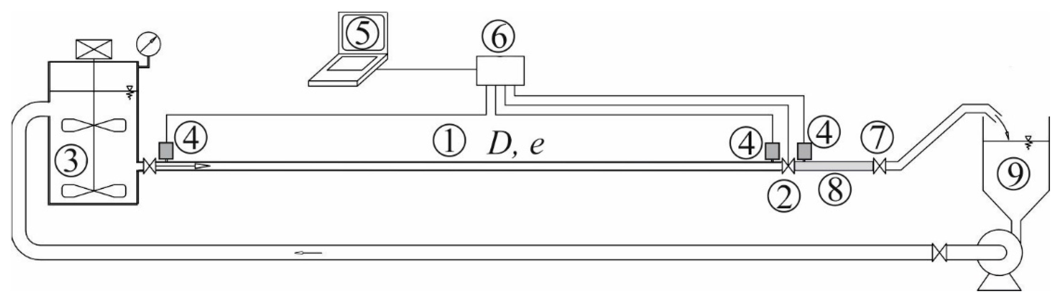
An experimental investigation of the pressure characteristics during transient liquid-solid flow was performed using the specially designed laboratory setup [30], shown in Figure 1.

The experimental rig consisted of a pressure tank and the high-density polyethylene (HDPE) pipeline (1) of 16.64 m in length, an internal diameter of 20.4 mm and absolute roughness of 0.04 mm. The homogenization of the slurry was obtained with the use of an axial stirrer in the tank (3). A compressor was used to maintain a steady value of the air pressure above the slurry surface in the tank.

At the downstream end of the HDPE pipe, a ball valve (2) was placed to provide rapid changes in the flow. The valve was equipped with a unique system registering the closing characteristics. The experimental data were collected with the use of three pressure transducers (4) (measuring ranges from −0.1 MPa to 1.2 MPa; measurement uncertainty 0.5%; linear performance characteristics; correlation coefficient R of at least 0.999). The transducers located at the upstream end of the pipeline and close to the valve (upstream and downstream, respectively) were connected to a computer (5) via an analog-digital card (20 MHz) (6). The signal from the transducers was sampled with a frequency of 2 kHz. An additional valve (7) was placed downstream of the ball valve (2) to ensure the desired constant value of discharge during the steady flow. Directly downstream of the ball valve, a short section of plexiglass pipe was installed (8) to enable observations of a flow during steady conditions. The discharge was measured based on the volumetric method with the use of a calibrated vessel (9). The slurry was pumped from the vessel to the pressure tank (3) via the return pipe. The geometrical dimensions of the model (raising the free liquid level above the axis of the discharge pipe is 1.5 m) prevented air from entering the pipe. Each of the experiments was proceeded by a prolonged flow in steady motion conditions and by venting pressure transducers several times.

4.2. General Course and Exemplary Results of Measurements

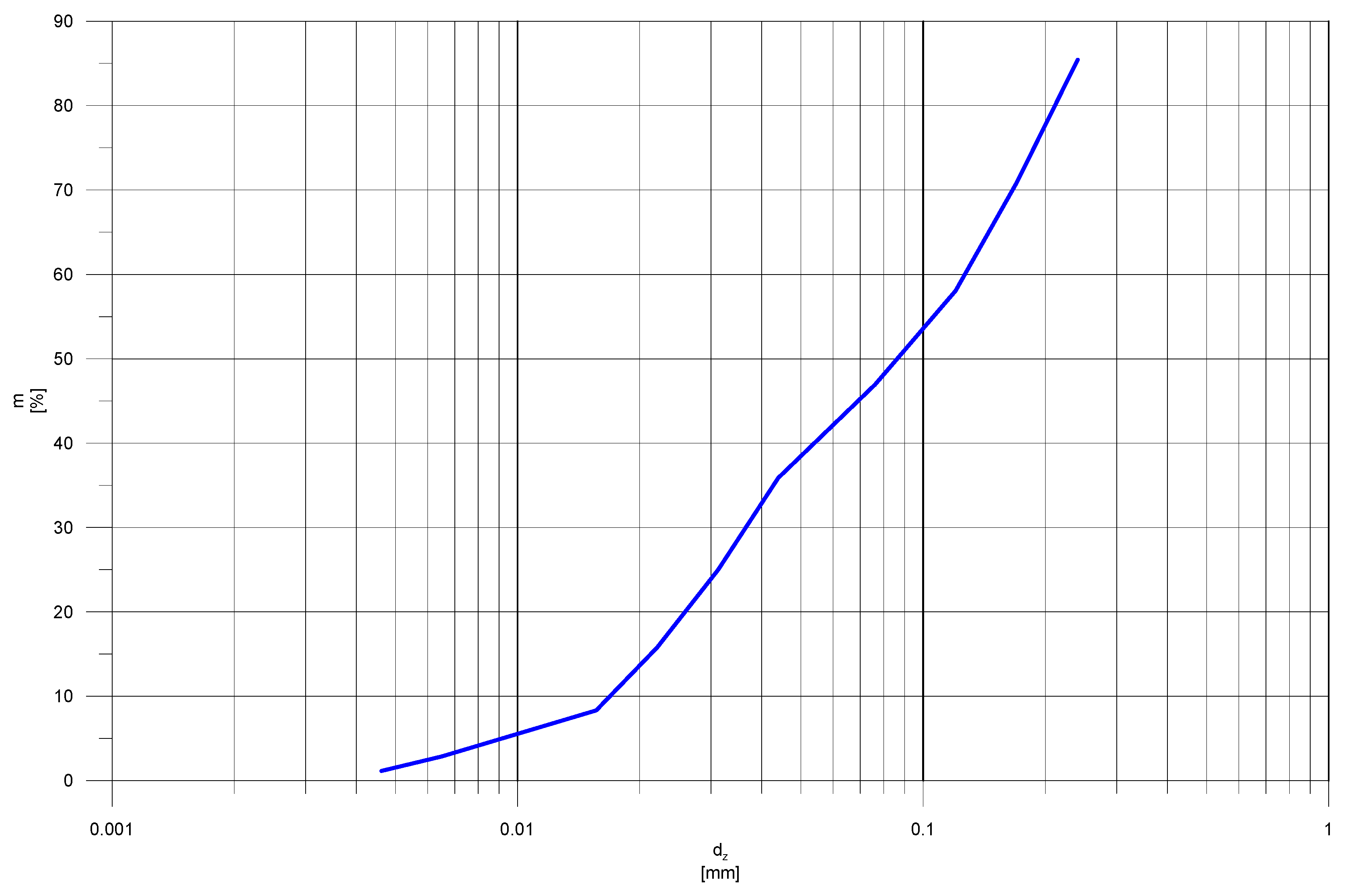
In the experiments, the mixtures of different slurry densities were considered. The mixtures were prepared with the application of the solid phase of the industrial slurry and water in varying proportions. The solid particles consisted mainly of small limestone grains. The solid material was taken directly from the existing slurry network. A grade curve of the used solid phase is presented in Figure 2.

In the preliminary phase of the experiments, the main parameters of the mixtures were determined. The density of the mixture and the solid phase alone was estimated based on a mass method. The average density of solids was 2715 kg/m³, and the densities of the mixtures ranged from 1012 kg/m³ to 1067 kg/m³, which corresponded to the volume concentrations C_V from 0.007 to 0.039.

Since the laboratory tests were conducted using an actual hydro-mixture consisting of water and finely ground limestone, the value of solid bulk modulus E_S was estimated based on the literature data, assuming relative elastic modulus E_S/E_L for limestone after [2], as equal to 43.0.

At the beginning of each experiment, the steady flow was considered. The values of the discharge and pressure in the tank and in the pipeline cross-section up to the valve were measured. The experiments on slurry flow were compared to the ones on water flow. In the next stage, the rapid water or slurry hammer was induced by the rapid closure of the valve (3). The pressure characteristics during the transient flow were measured. Several experiments with different steady-flow average velocities (vav) were conducted for each slurry concentration and water. Based on each pressure characteristic, the maximal empirical pressure increased, and the empirical water or slurry hammer period temp was determined. Consequently, the empirical wave celerity was estimated based on the formula:

$$a_{emp}=\frac{4L}{T_{emp}}$$

(12)

where L is a length of a pipeline.

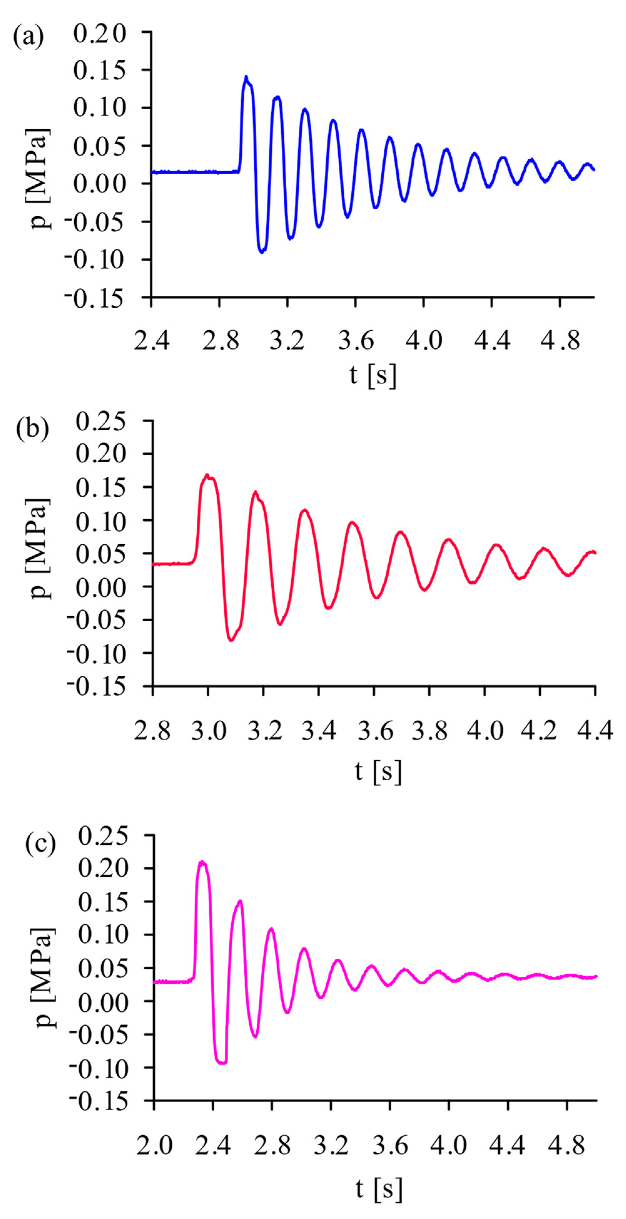
The exemplary results in the form of pressure characteristic obtained for similar v_av (~0.3 m/s) for water (ρ = 1000 kg/m³) and slurries of two different concentrations (slurry 1: C_V = 0.007, ρ_m = 1012 kg/m³; slurry 2: C_V = 0.039, ρ_m = 1067 kg/m³) are presented in Figure 3.

4.3. Results and Discussion

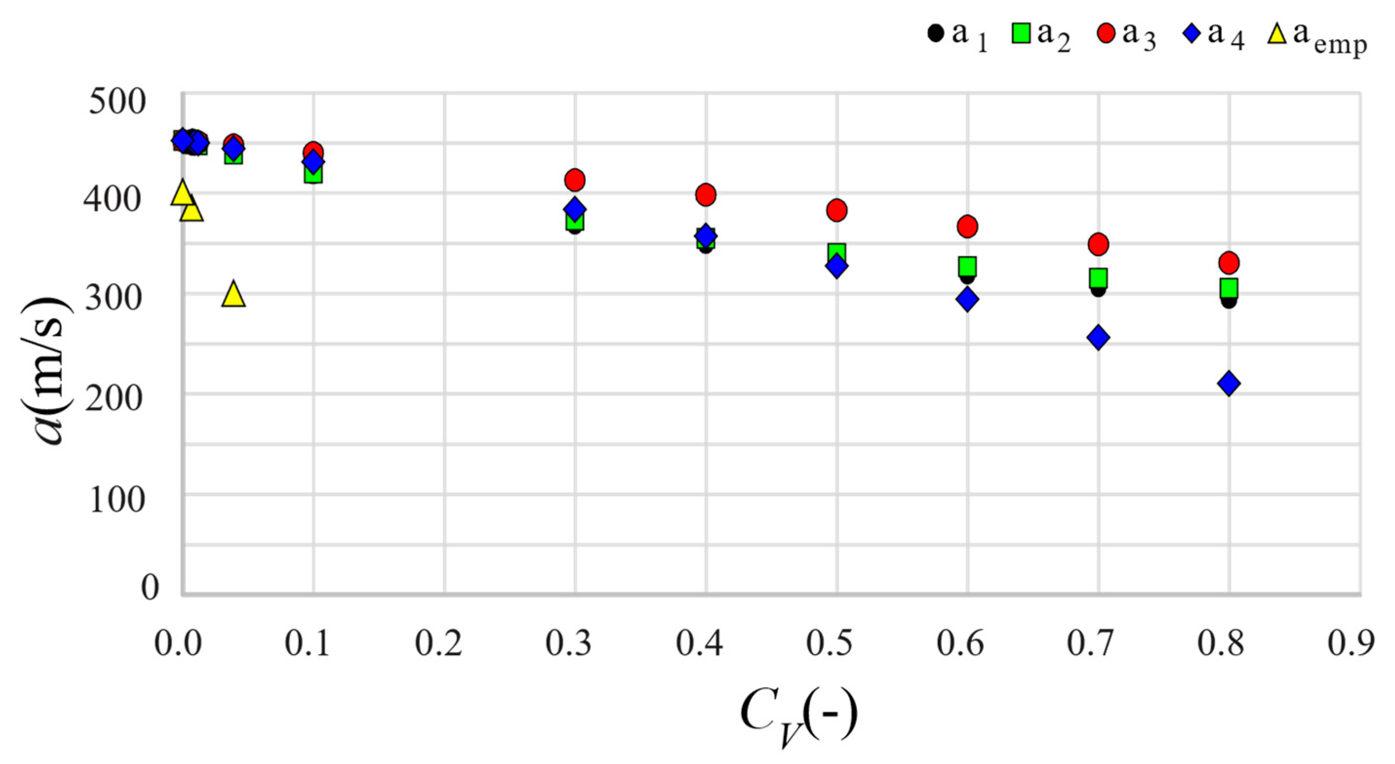
The sludge used in the research was a two-phase mixture with a low concentration of solid particles. Therefore, from a computational point of view, it could be treated as a homogeneous mixture. However, observations of the behavior of solid particles during steady flow, carried out thanks to the transparent section of the pipe (8), showed that even at such low concentrations, the solid particles tended to settle and create a small bottom layer. It is, therefore, interesting if the homogeneous model is still appropriate in the considered case and to what extent the available theoretical formulas for wave celerity correctly reflect the real values observed during the experiments. Thus, the values of wave celerity a₁, a₂, a₃ and a₄ were calculated with the use of the Equations (8)–(11) and compared with their experimental equivalents a_emp. Additionally, for a better comparison of theoretical values in a wider range of concentrations, a few hypothetical slurries were also considered. Exemplary values are presented in

Table 1. Main parameters of selected experiments.

Fluid	ρm (kg m−3)	CV	Wave Celerity (m/s)
			a1	a2	a3	a4	aemp
Water	1000	0.000	452.2	452.2	452.2	452.2	401.0
Slurry 1	1012	0.007	449.6	449.7	451.4	450.8	385.0
Slurry 2	1067	0.039	437.8	438.6	447.4	444.1	300.0
Slurry 3 *	1172	0.100	417.8	419.7	439.7	431.0	—
Slurry 4 *	1686	0.400	348.3	354.8	398.3	356.8	—
Slurry 5 *	1858	0.500	331.8	339.6	382.9	327.3	—

Note: * hypothetical slurry.

and in Figure 4.

The preliminary analysis allows us to conclude that in the considered case, none of the theoretical formulas satisfactorily reproduce the actual values of the wave celerity observed during the experiment. Experimental values were significantly lower than theoretical ones, and the discrepancy increases with the increase of C_V. That suggests that the actual course of analyzed phenomena is much more complex than the models adopted for deriving theoretical formulas.

One of the factors modifying the course of a water or slurry hammer in the considered case is the pipe material. Polymer pipes demonstrate viscoelastic properties, which is a significant difference in relation to the elastic conduits, for which theoretical formulas were historically derived. However, this is not the only reason for incompatibility of the results of calculations with observations, especially in the case of slurries. Thus, the question arises whether, despite the complexity of the problem, it is possible to effectively reconstruct the course of the phenomenon on the computational path, to obtain a satisfactory agreement between the results of calculations and observations while the relative simplicity of the computational model. Numerical experiments were carried out for this purpose.

5. Numerical Simulations

5.1. Numerical Model

In the study, the applied numerical model of transients in slurries at low concentration was developed based on the assumption that the solid-liquid mixture may be treated as a pseudo-homogeneous medium, with the fixed, averaged in the cross-section and constant in time and space parameters (density and viscosity) that were specified for the slurry treated as pseudo-liquid. The model enabled the computational simulation of pressure changes in the pipeline. Consequently, the cross-sectional area of the slurry stream is equal to the cross-section of the pipe, with no solid bottom layer. Unsteady flow during water/slurry hammer can be further described using a one-dimensional system of partial differential equations governing the transient flow of compressible fluid in viscoelastic pipe Equations (1) and (4).

While adopting the numerical model to the considered case, the following additional assumptions have been made:

• Wave celerity during each episode of water or slurry hammer remains constant;
• Viscoelasticity of the pipeline material is described with a one-element Kelvin-Voigt model with two parameters—retardation time and creep compliance;
• Initial values of pressure and velocity along the pipeline were calculated based on the steady flow equations, with boundary conditions defined by the measured values of steady-state discharge and pressure in the reservoir;
• Boundary conditions were defined as constant pressure values in the reservoir (upstream condition) and the valve closure function (downstream condition).

Traditionally, the method of characteristics is commonly used to solve the system of equations of transient flow. However, it has been proved (e.g., [31]) that due to the properties of this method, the solution is significantly sensitive to the non-physical effects generated by the numerical scheme. Such effects produced during the computational process may significantly affect the solution, making its proper interpretation difficult. Considering this, a numerical solution in the analyzed case was performed with the use of the finite difference method. The absolutely stable four-point scheme was applied. The values of the numerical parameters were adopted to ensure absolute stability and maximal accuracy of the scheme. In each episode, the optimal time step Δt was determined considering the value of the pressure wave speed to obtain the value of the Courant number as close to unity as possible.

Identification of the parameters characterizing the viscoelasticity of the pipeline material was developed according to the procedure presented in [21] or with the trial and error method.

5.2. Numerical Results and Discussion

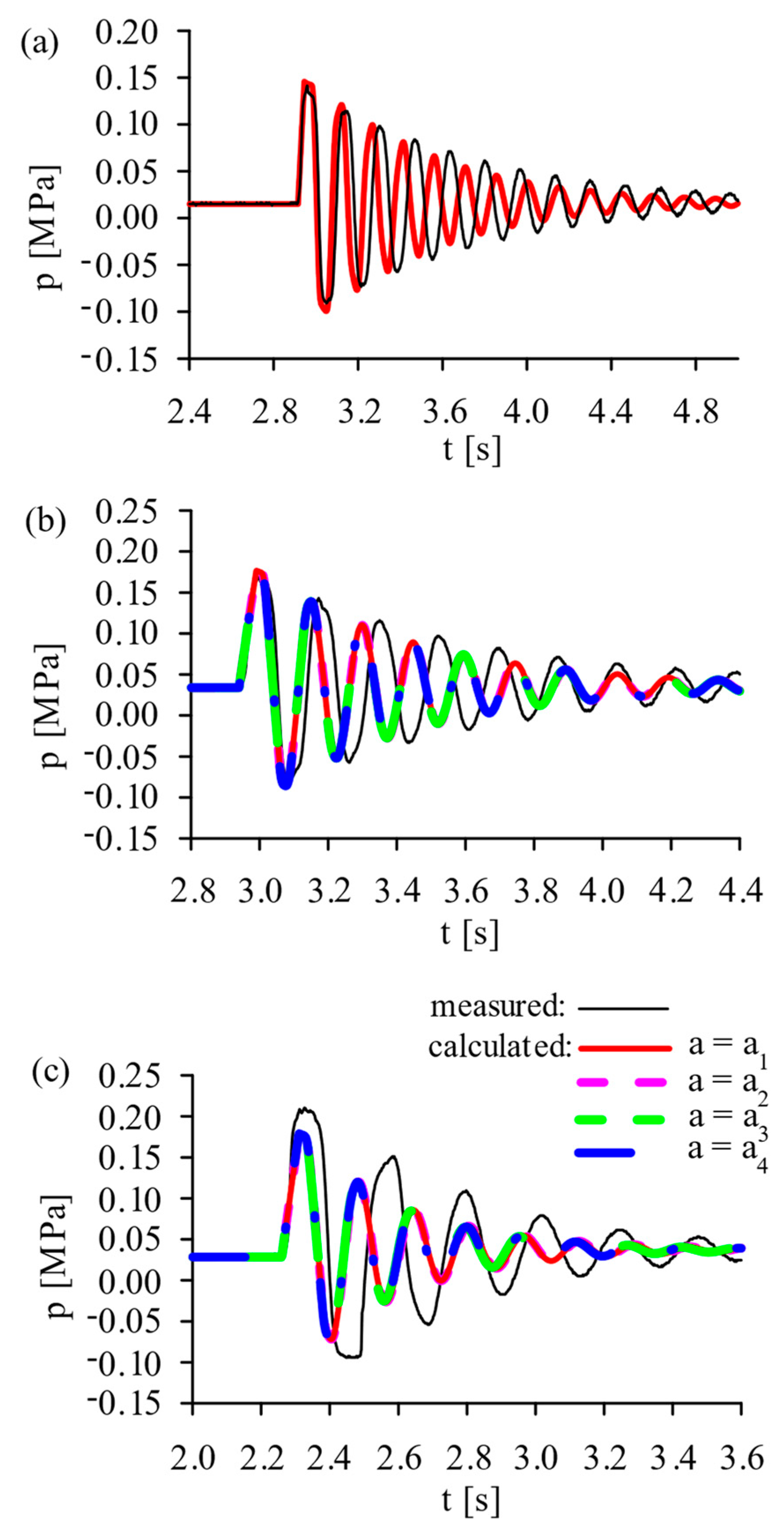
The previously analyzed cases of water and slurry flow were used to compare the results of measurements and the numerical calculations. In the first stage of numerical calculations, the values of wave celerity a₁ ÷ a₄, estimated on the base of theoretical formulas Equations (8)–(11), were applied to conduct the numerical solutions for each analyzed case. The exemplary pressure characteristics compared to experiments are shown in Figure 5.

The pressure characteristics calculated with the use of theoretical values of wave celerity were very similar, but they showed significant non-compliance with the measured ones. Both the frequency of oscillations and their amplitude clearly differed from those observed, and the differences increased with increasing C_V. The differences between the characteristics obtained for different theoretical formulas for the wave speed differ to a negligible degree only and were irrelevant to the quality of the solution in the considered case. None of the analyzed theoretical formulas leads to a satisfactory result.

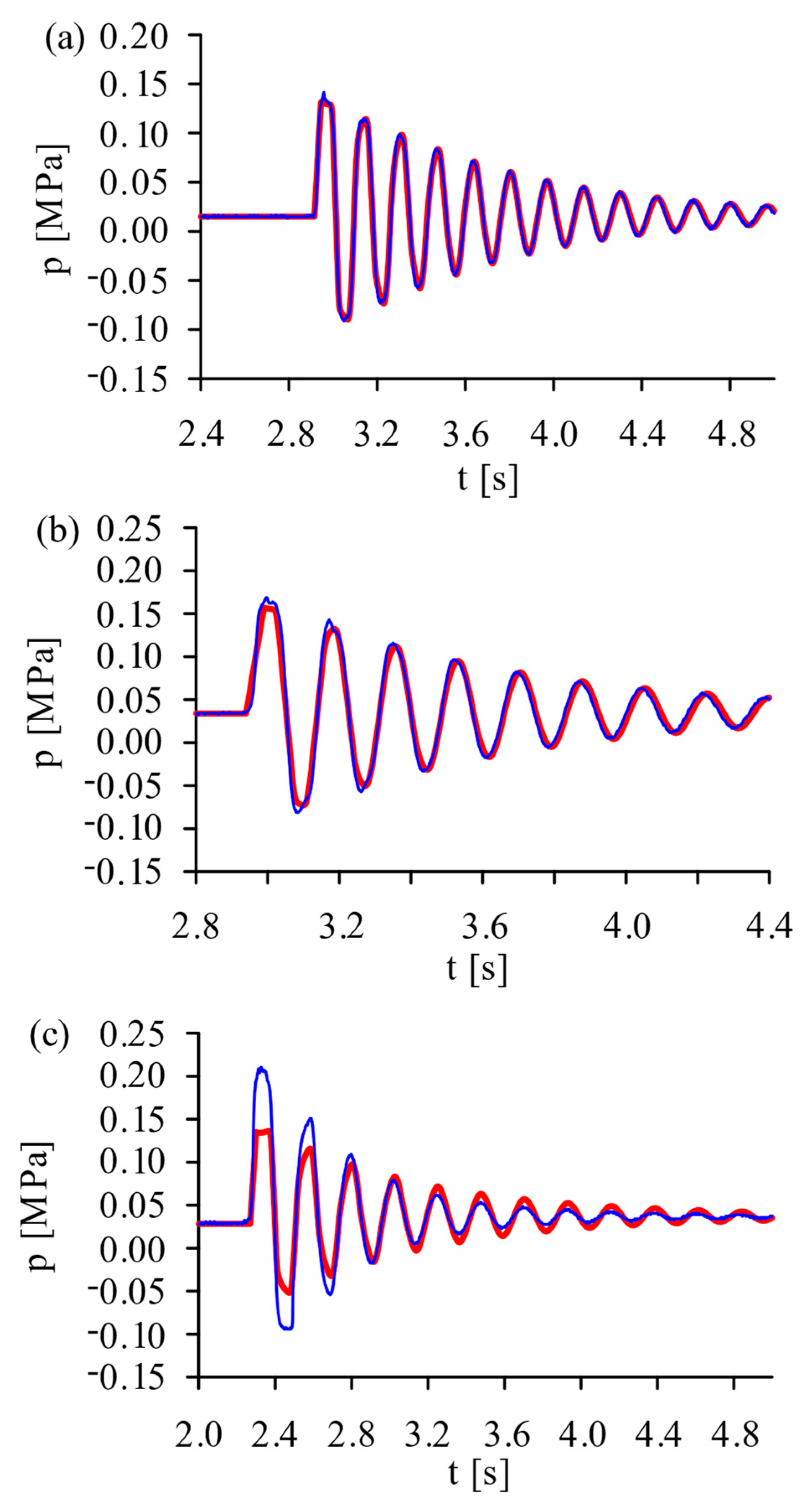
In the next stage, the calculations with the experimentally obtained values of wave celerity a_emp were conducted. The exemplary results are shown in Figure 6.

In this case, the calculated pressure characteristics demonstrated much better compliance than the experimental ones. In the case of water, the calculated and measured pressure values were consistent. Both the oscillation frequency and maximal pressure increase observed during the experiments were successfully reproduced in calculations. In the case of the slurry, good compliance of calculated and oscillation frequency was still observed in all analyzed cases. However, the calculated pressure values, although still acceptable for very low concentrations, demonstrated a significant discrepancy when slurry concentration increased. The calculated values were too small in the first few amplitudes of the oscillations while too high in the continuation of the phenomenon. This fact indicated that the simplified model used so far reproduces the rate but is not able to correctly reproduce the intensity of pressure damping during transient flow. The observed slurry hammer showed greater dynamics–higher pressure increases and more intensive damping of oscillations. This fact is partly confirmed by [2], who found that the total change in pressure values during the slurry hammer is the result of the overlapping of two waves–the liquid phase hammer (also called the initial hammer) and the particle hammer, the latter being considered negligible in most engineering cases. Obviously, the two interfering waves cannot be physically reproduced with the model assuming a pseudo-homogeneous mixture. However, it is worth noticing that the desired effect of higher dynamics in pressure damping was similar to the result of a slurry hammer in the pseudo-homogeneous mixture of increased density. This analogy enabled further modification of the computational model by the concept of equivalent density.

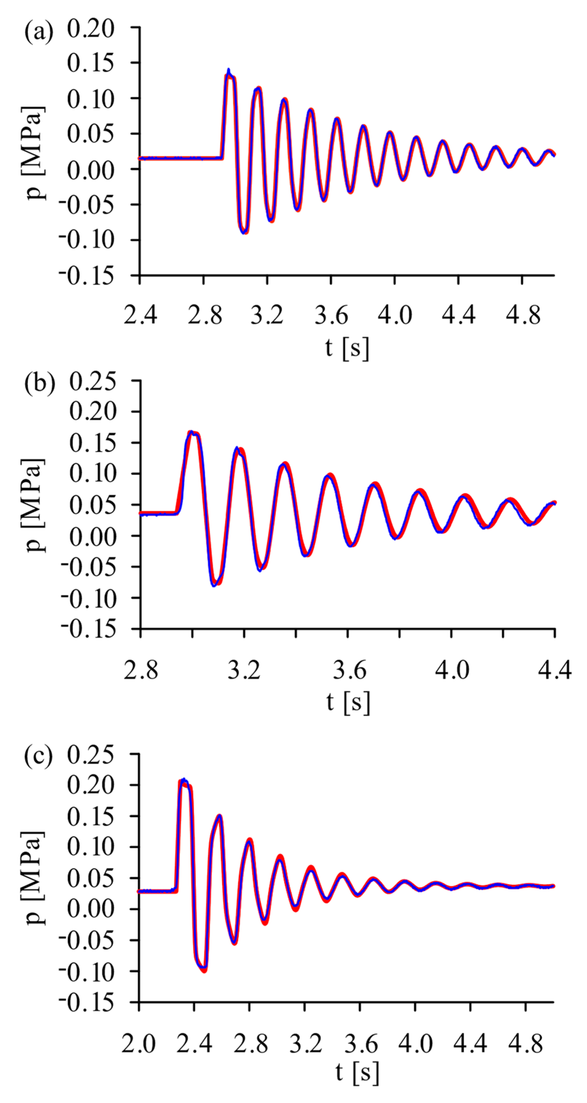
The equivalent density ρ_eq was applied in transient flow equations instead of mixture density ρ_m. It could be treated as a conceptual parameter representing all the additional mechanisms affecting the pressure wave oscillations, including the existence of the bottom layer. The value of ρ_eq was thus dependent on the type and size of the particles, slurry concentration and flow velocity. It increased with the concentration increase and steady-state velocity decrease. In the considered slurry hammer cases, the values of ρ_eq were estimated during model calibration as equal to 1076 kg/m³ and 1790 kg/m³ for the slurry of C_V, equal to 0.007 and 0.039, respectively. The exemplary results are shown in Figure 7.

As can be seen, a significant improvement in consistency with the experiments was observed. Both the rate and the intensity of damping of the oscillations were correctly reproduced in calculations. In all considered cases, the simplified computational approach combined with the equivalent density concept enabled obtention of satisfactory complied calculated and observed pressure oscillations.

6. Summary and Conclusions

Transient flow in slurries has a complex course, and it is very demanding to describe in an accurate way all the mechanisms accompanying the flow. The main reasons for this fact are the unsteady nature of the phenomena and spatial variability (both within the cross-section and along the stream) of the main parameters and quantities characterizing the flow. On the other hand, the occurrence of transient, including a slurry hammer, plays an important role in hydro-transport systems and should be considered during their dimensioning and operation.

From a practical point of view, the most important issues related to transient flows in pipelines include the correct assessment of extreme pressure values–both in terms of identifying critical localizations in the industrial system where the phenomenon may appear, as well as determining the maximum and minimum pressure values that may pose a threat to proper system operation and safety. Focusing on the system protection, these issues are crucial, while the problem of correct reproduction of other flow characteristics (e.g., velocity distribution, diversification of concentration, bottom layer thickness, etc.) is shifting to the background. In such situations, it is important to develop a computational model that will enable the reproduction of pressure characteristics in different flow conditions and predict the extreme values in the correct way, with the simultaneous relative simplicity of mathematical description leading to the reduction in the number of model parameters that are difficult to identify.

In this study, an alternative, simplified and effective approach to the mathematical description of the unsteady slurry flow was applied. The presented model, based on a quasi-homogeneous mixture concept with modified parameters, may be used in the cases of both elastic and viscoelastic pipeline materials. Regarding the quick development in technology and a distinct tendency to use polymer materials in various pipeline systems, this modification was an important feature of the model. The description of the mixture properties was simplified, which reduced the number of parameters that should be identified. This facilitated a mathematical description.

The simplified computational model applied in this study proved to be effective for the purpose of correct reproduction of the pressure characteristics during unsteady flows of low concentration mixtures. As a basis for the analysis, a series of experiments were conducted. The results of the calculations, compared with the experiments, showed high compliance, thus suggesting that the proposed approach may be a promising solution for the analysis of slurry hammers in industrial systems, enabling the application of the method. However, it turned out that both theoretical formulas for the wave celerity during slurry hammer and the classic approach to defining the density of the mixture did not allow satisfactory results in this case. The empirical wave speed observed during experiments was lower than the values obtained from theoretical formulas, even those including the heterogeneous nature of the mixture. Moreover, the observed pressure characteristics indicated that a higher value of mixture density, compared to the classical approach expressed in Equation (6), should be adopted in the simplified model. Thus, the concept of equivalent density was applied. The equivalent density may be treated as a conceptual parameter representing in one value all the mechanisms affecting the pressure wave oscillations, which were not explicitly considered in the simplified mathematical description. This parameter was also related indirectly to the depth of the bottom layer. The value of equivalent density was thus dependent on the type and size of particles, slurry concentration and flow velocity. It increased with the mixture concentration increase and the steady-state velocity decrease. Both parameters, empirical wave velocity and equivalent density should be determined based on measurements during model calibration.

The introduction of the two previously mentioned parameters into simplified mathematical equations led to the successful reproduction of pressure characteristics, both in relation to the frequency of oscillations and the rate of their damping. Satisfactory results allowed us to conclude that, at least in relatively low concentrations, the proposed approach could be an interesting alternative to much more complex computational models requiring the identification of a much larger number of variable parameters.