Flexible Low-Carbon Optimal Dispatch of Honeycombed Active Distribution Network

Abstract

Microgrids have a strong ability to generate local power and consume renewable energy, which can solve the problems of power supply shortages and greenhouse gas emissions created in the process of social development. The honeycombed active distribution network (HADN) can flexibly, independently, and interconnectedly operate microgrids through power exchange stations, so appropriate HADN dispatch can produce increased low-carbon benefits than general microgrids. In this study, we first designed a model for optimizing HADN with the lowest carbon emission as the target, then we introduced the concept of carbon emission flow into the optimization process to determine the carbon emission level of each element. Finally, we illustrated and verified the proposed model by a HADN composed of three microgrids. The optimization results of the case study showed that by scheduling the DGs within the microgrids, the total carbon emissions of the system were reduced from 123,328.1 to 117,688 kg CO${}_2$; the system with a HADN structure was able to produce only 110,958 kg CO${}_2$ and effectively reduce carbon emissions by 10%, which proved that HADN can be scheduled with high flexibility and provides increased low-carbon performance through the proposed optimization dispatch method.

1. Introduction

With the development of science and technology, modern lives are increasingly complex, thereby requiring a large amount of resources to support. With this huge requirement for resources, energy and environment problems have become increasingly serious, challenging the further development of human society. Against this background, most nations have decided to consider dramatically reduce their greenhouse gas (GHG) emission while planning the development of their economy and other aspects. Specifically, the transfiguration of electric power systems is being prioritized because electric power has historically been the most important energy form; almost all of the serious effort to pursue carbon reduction requires the support from the corresponding electronic power systems. Most of the GHG emissions are generated by the burning of fossil fuels; thus, curbing the use of fossil fuels and finding alternative energy resources are two key issues to address the energy and environmental problems [1].

In recent years, the development of renewable energy generation (REG), for example, wind power, photovoltaic power, and hydrogen fuel cell generation, has pushed the generation of power systems to undergo deep transformation from centralized to distributed generation [2,3]. That is, more and more small- and medium-scale REG plants are being connected to power systems, especially in distributed power systems. REG plants have also produced significant challenges for the planning and operation of power systems while generating electricity, because of the randomness and uncertainty of REG [4]. In power systems, the generated power must be balanced with the load; otherwise, the frequency and voltage shift far from normal values, which causes outages and other faults in power systems. However, the power generated by the REG cannot be chosen by humans, as it is related to the conditions in nature, e.g., wind speed, so it is hard to ensure balance in power systems with a high penetration of REG.

In order to solve the power balance problem in distributed power systems with a high penetration of REG, some scholars put forward the concept of microgrids, in which distributed generators (DGs), energy storage units (ESs), various alternating current (AC) and direct current (DC) user loads, and related control and protection devices are combined to form a small-scale power system with independent operation capability [5,6,7]. Compared with traditional distribution power systems, microgrid-based distribution power systems are smaller and simpler in structure, easier to control, and have a stronger ability to realize local power generation and consumption [8]. Thus, microgrids provide a powerful tool to address the challenges produced by a high penetration of REG. However, microgrids usually have a limited capability to adjust their power generation to ensure the power balance; thus, they usually require the support of other sources, for example, another microgrid or a main power system. Therefore, with the development of microgrids in distribution power systems, microgrid technology has gradually developed from a single microgrid to multiple microgrids. Furthermore, because of there are many types of generators and power supplies connected to different microgrids, the GHGs emitted by different generators are different from each other, so with different power generation profiles, the GHG emissions of the whole system also differ. Thus, with multiple microgrids, the carbon emissions of the whole system can be optimized. This feature of multiple microgrids makes them outstanding as an attractive potential solution for a low-carbon distribution power system with high a penetration of DGs and ESs [9].

With the development of the multiple microgrid structure in distribution power systems, the honeycombed active distribution network (HADN) was proposed as a structure for unifying multiple-microgrid-based distribution networks, which is based on a topology adapted for the large-scale application of microgrids [10]. In HADN, considering the power and information interaction between microgrids, each microgrid is interconnected through a power exchange station (PES). The interactions of geographic connections and power information in microgrids are enhanced by linking neighboring microgrids together through PESs [11]. The reliability of the HADN was evaluated, and a mathematical model for the simulation of the reliability of the HADN was constructed using the Markov process to verify the high power supply of the HADN reliability [12]. In the study of the strategy for controlling this topology, Refs. [13,14] conducted normal operating condition power balance analysis, fault isolation and stability analysis during abnormal operating conditions, and proposed a control strategy for HADNs. Ref. [15] studied its optimization scheduling problem, selected the minimization of operating costs as the optimization objective, used the distributed optimization method based on the consistency constraint for optimal scheduling, and analyzed the impact of the application of HADNs on the economy and reliability of microgrid groups.

To analyze the direction of carbon flow between system microgrids and the division of carbon emission responsibility, the concept of carbon emission flow intensity (CEI) was proposed for the low-carbon analysis of power grids, providing a new perspective for the analysis of low-carbon power systems [16,17]. The theoretical systems, and methods of analysis and calculation of carbon emission flow have been further improved and verified by various types of transmission systems, and the real-time carbon emission flow intensity (CEI) of any node of a system can be obtained according to any known system power distribution [18,19,20,21,22]. In recent years, this concept has also been gradually introduced in grid carbon emission analysis and optimization scheduling.

Releated Work

Research on low-carbon optimization of power grid has been increasing in recent years.

Ref. [23] used the hourly power production of DER and the hourly storage unit level to minimize the annual cost of generators, carbon emissions of the overall system, and line losses.Through the multiobjective approach based on nondomination, the problem of the 24-hour unit commitment of DGs to supply a microgrid connected to the main grid was addressed.

Ref. [24] presented a new emission-constrained power-generation expansion model to meet emission targets. These researchers considered REG and evaluated the year-round generation and emission cost using a dynamic programming based unit commitment. They finally provided the optimal results and studied the variation in generation costs for different emission prices.

Ref. [25] presented a novel model of a low-carbon distribution network containing microgrids, which considered different GHG emission levels and the generation costs of various distributed power generation types. At last, using the chaotic ant swarm algorithm, the simulation results showed the correctness and validity of the model considering different prices of CO${}_2$ emissions.

Ref. [26] proposed a model for analyzing electricity production and storage in a microgrid, with the goal of satisfying load demand at minimal production costs and CO${}_2$ emissions. The paper presents the results of a simulation of the production and storage of electricity in a microgrid that was part of a distribution network.

Ref. [27] proposed an optimized dispatch model, which considered the carbon capture device and wind power plant. The model was solved by the binary DE-BBO algorithm and the minimum marginal cost method. The proposed model could enable low-carbon dispatch with remarkable energy-saving efficiency.

Ref. [28] established a CEF analysis model of ESs, based on which the low-carbon optimization operation model of a distribution network with the lowest carbon emission as the objective function was established. The model provided an effective reference for establishing the low-carbon optimization operation method of power distribution networks.

Ref. [29] established a modified low-carbon economic dispatch model for integrated energy systems, which is based on CEF for an energy hub and carbon trading. Carbon trading cost was considered in the optimal economic dispatch, and the case study of models indicated that the proposed model more stringently controlled carbon emissions.

Table 1. Summary of related studies.

Reference, Year	Objective	Unknowns	Solving Method	Test System
[23], 2010	To minimize annual cost, carbon emissions and line losses	Output power of DERs and storage unit level	NSGA-II	A MV microgrid
[24], 2011	To minimize fuel and aggregated costs	Output power of DERs	Enumeration method	IEEE 30-bus system
[25], 2012	To minimize generation and emission costs	Output power of DERs	Chaotic ant swarm Aagorithm	A distribution network containing microgrids
[26], 2013	To satisfy load demand at minimal production costs and emissions	Power production and storage	FICO Xpress	A microgrid system
[27], 2015	To minimize the total cost including the cost of carbon emissions	The output power of DERs	Binary DE-BBO algorithm	IEEE-RTS 24-bus system
[28], 2019	To minimize carbon emissions of the system	Power production and storage	CPLEX	IEEE 33-bus system
[29], 2019	To minimize IES outsourcing energy and carbon trading costs	Output power of DERs	Gurobi	An IES containing CCHP

summarizes the related studies we selected in this research. It is essential to highlight the evolution of studies on optimization problems, which are made flexible through the use of configurable variables and are dispatchable for the development of demand; thus, they able to be used to reconfigure power generation portfolios, thereby contributing to the concept of a low-carbon grid. However, the above low-carbon optimization operation methods were all applied to traditional distribution networks or small microgrids. Because the process of optimizing HADNs needs to consider the power exchanged between different microgrids through PESs, the optimization model is different. Additionally, optimization with the goal of low-carbon emission requires a real-time calculation of the CEI of each microgrid to control the direction and magnitude of the power flow. The conventional optimization methods are not applicable to HADN, so this gap still exists. In this study, we addressed this gap, which reflects the innovation and importance of the research presented in this paper.

As a large number of DGs and ESs can be connected to a HADN, and the unique configuration of a HADN allows for flexible power dispatch, ensuring that it can dispatch power sources according to the low-carbon level of power generation, HADN has advantages in low-carbon operation. Therefore, a low-carbon optimization method for HADN is urgently needed to fully achieve its low-carbon performance. The main objective of the optimization dispatch model in this study is to reasonably reduce the carbon emissions of a HADN by scheduling the power output of the main grid, DGs, and ESs, as well as the charging and discharging power direction and size of the ES sat PESs. The whole model is divided into two parts: the microgrid and PES parts. According to the carbon emission intensity (CEI) of different power generators, general software is used to solve the optimization model. The PES part is performed by formulating the charging and discharging rules of the ESs related to carbon emissions. We specifically designed the PES-microgrid transmission factors for the power transmission problem between PESs and microgrids by using the CEI node obtained from CEF analysis theory. Finally, the model was validated on a HADN consisting of three microgrids. The optimization results proved that through the optimization dispatch established in this study, the HADN can not only reasonably arrange the power output of the DGs inside the microgrids, but also coordinate the low-carbon power dispatch among the microgrids. Compared with other types of distribution networks, the HADN produces the best low-carbon effect and can be flexible in inter-regional power dispatching according to the optimization target.

The rest of this paper is organized as follows: Section 2 describes the structure and features of HADN, and the definition and calculation of the CEI. Section 3 establishes the model of the low-carbon optimization dispatch of the HADN. Section 4 presents the numerical evaluation and discussion of the computational results, then analyses the flexibility of the dispatch of HADN. Finally, the conclusions of this study are given in Section 5.

2. Overview of HADN and CEF

2.1. HADN Structure and Features

As shown in Figure 1, a HADN is constructed with two fundamental parts: the active microgrids and the PESs. Each microgrid is connected to the PES through the common connection point (CCP) to exchange power between the microgrid and PES. Without loss of generality, the topology of the microgrid is abstracted into the hexagon with the PES located at the six corners of the hexagon, as shown in the figure.

The PES contains the circuit breaks, busbar integration, power electronic converters, and energy storage unit to support the power connection and energy storage function of the power system operator. With circuit breakers and a DC/DC converter, the PES can be connected to different microgrids with different voltage levels and support a controllable power flow path between the connected microgrids. The structure of the HADN provides a flexible solution to the challenge created by the high penetration rate of renewable energy. The active microgrid shown in Figure 1 can be operated in grid-connected or island models. Each active microgrid can adopt multiple-voltage-level AC, DC, or mixed AC/DC distributions. Under normal conditions, the power supply and load within each microgrid are self-balancing. When there are power fluctuations or dispatching by the decision center, the power is exchanged with neighbor microgrids through PESs to achieve dynamic balancing.

Compared with other existing distribution networks, HADNs have the following advantages:

(1) High controllability, stronger grid distribution structure, and the failure of one microgrid does not affect the normal operation of the other microgrids. The traditional grid structure of an active distribution network is determined through a large area network power supply method, where any fault may affect other areas, which may cause systemic instability collapse and large blackouts in serious cases. In contrast, each microgrid in a HADN autonomously operates and interconnects with the others through PESs. When any microgrid fails, all PESs can quickly determine and cut off the power connection channel between them, thus isolating the microgrid from the distribution network, ensuring a strong and intelligent distribution network.

(2) In HADNs, each microgrid has six associated PESs to provide active support and auxiliary balance regulation, which effectively improves the operational stability and power supply reliability of the system.

(3) HADNs have good scalability and easy design and conversion. The traditional distribution network is difficult and costly to expand and renovate, often requiring new system design, equipment capacity accounting, et.. HADNs consist of a standard configuration of microgrids that are organically connected together through PESs, so distribution network planning and design, construction, and renovation are easy.

(4) The marketization of electric power is easier. The traditional distribution network adopts large regional network power supply method, which has strong natural monopoly property and is not conducive to power market reform. HADN realizes microgrid autonomous power supply, and the operation of each microgrid is relatively independent, so it is easier to realize power marketization.

(5) The property of HADNs that best fits the low-carbon scheduling problem in this study is their strong capacity to handle the high penetration rate of renewable energy. With increasing penetration of renewable energy generation, the stability and reliability of traditional distribution networks have become worse because they cannot flexibly control the power flow to deal with the random fluctuations in the generated active power by renewable energy. Thus, compared with traditional distribution networks, HADNs have a much more flexible structure. The microgrids in a HADN construct a relatively independent micropower system, and the generated DG can be first consumed in the local area, and the unbalanced power can be transported to other microgrids and the ESs in the PESs to overcome the power unbalance issue. Thus, the interactions of different microgrids with the ESs in the PESs make HADNs much more suitable for the integration of REG. Additionally, the HADN topology has a large number of ESs, which require little energy storage and a relatively simple model, thereby considerably reduces the construction cost of the microgrids.

The traditional distribution network has a single source of power and a constant tidal path direction. The source of electrical energy for the ES is also fixed. In comparison, HADNs have the following features for power path control: The ESs in the PESs have peak-shaving and valley-filling effects on the CEI. When the microgrid is in low-carbon operation, the ESs absorb low-carbon power from the microgrid through CCP. When the microgrid enters a high-carbon operation period, the ESs can release low-carbon power to the microgrid. Normally, one PES can connect up to three microgrids, and there are more than one PES in a HADN, so HADNs are networks with deep crossovers. In summary, because of the above features of HADNs, the PESs can find the lowest-carbon intensity source to release active power, which means that it can achieve the lowest carbon emission operation of the system. HADNs are also suitable for the facilitation of the reasonable distribution of low-carbon emission targets among microgrids in each region. In order to cope with the situation in which a microgrid has the lowest CEI, the charging and discharging rules of the ESs of the PESs can be artificially adjusted to change the electric energy path in order to balance the carbon emission responsibilities between regions and ensure the overall reasonable operation of the distribution system.

As shown by the analysis above, HADN has advantages in flexible low-carbon operation. So, the main objective of optimization dispatch in this study was to reasonably reduce the carbon emissions of a HADN by scheduling the power output of the main grid, DGs, and ESs, as well as the charging and discharging direction and power of the ESs in the PESs.

2.2. CEF Definitions

The concept of CEF proposed in [17] was introduced for the optimization of low-carbon emissions in the HADN to quantify the attribution of carbon emission responsibility within and between different microgrids. The calculation of CEF is often accompanied by the calculation of power flow. The carbon emission of branch flows from a node is equal to the CEI of the node, which is used to derive a solution to the CEF distribution of the power system under any power flow distribution. The definitions and calculations of the relevant physical quantities were detailed in [18], and are organized in

Table 2. Physical quantities of CEF theory.

Physical Quantity	Meaning	Calculation Formula
Branch CEF (F)	Amount of carbon emission flow on the branch
Branch CER (R)	Carbon flow rate of a branch that passes with the power flow per unit time t	$R=\frac{dF}{dt}$
Branch CEI ($\rho$)	Ratio of branch carbon emission flow rate to active power P	$\rho =\frac{R}{P}$
Nodal CEI (e)	Equivalent carbon emission value on the generation side caused by a unit of electricity consumed at the node	$e=\frac{{\sum }_{i=1}^N{P}_i{\rho }_i}{{\sum }_{i=1}^N{P}_i}=\frac{{\sum }_{i=1}^N{R}_i}{{\sum }_{i=1}^N{P}_i}$

.

The carbon emissions of a traditional network are only related to the CEI of the main grid, DGs, and ESs, if the structure of the system remains unchanged, because the CEI of each node is only related to the branch carbon emission flow rate and active power flowing into that node, which are determined by the power flowing into the network from the sources. Therefore, if the discharge CEI of each source is known, the reasonable arrangement of the power output of each source can be used to adjust the carbon emissions of the system.

It is necessary to pay special attention to the CEI of ESs because it is not a constant value and is determined by the charging and discharging process. When the ES is charged, the process of accumulating power is also the process of accumulating CEF, and the ES can be regarded as a load. When the ES is discharged, the process of discharging is also the process of injecting the carbon flow previously accumulated back into the power system, and the ES is regarded as a generator. Thus, when calculating the CEF of a distribution network with ESs, there is a parameter that needs to be calculated. The discharge CEI of the ES when it switches from charging to discharging state after the Nth charging period, $e_{ES\left(N\right)}$, is calculated as Equation (1), which indicates carbon emissions per kilowatt of electrical power. It is based on the remaining power and carbon flow rate of the ES at the last change from the discharged to the charged state (moment $T_0$, $Q_0$, and $F_0$), the conversion efficiency of the ES charging and discharging process, $\eta$, the charging power and carbon intensity at the ith charging period ($P_i$ and $e_i$), and the period length, $\mathsf{\Delta }t$.

$$e_{ES}\left(N\right)=\frac{1}{\eta }\frac{F_0+{\sum }_{i=1}^N{P}_i{e}_i\mathsf{\Delta }t}{Q_0+{\sum }_{i=1}^N{P}_i\mathsf{\Delta }t}$$

(1)

3. Proposed Low-Carbon Optimization Method

The whole model is divided into two parts, the microgrid and PES parts. According to the carbon emission intensity (CEI) of different power generators, general software is used to solve the optimization model. The PES part is dispatched by formulating the charging and discharging rules of the ESs related to carbon emissions. Optimization is mainly focused on the microgrid part; the considered inequality constraints are the generating unit capacity limits, while the equality constraint is the generation–demand balance.

3.1. Objective Function

The objective of optimization is to minimize the carbon emissions of the system, which is defined as Equation (2). $f_{SG}$ is the total carbon emission of the system, where each multiplication element corresponds to the carbon emissions emitted by each source. $P_{GRID,t}$ is the power from the superior main grid at time t, $P_{DG,k,t}$ is the power emitted from the DG k within the microgrid at time t, $P_{PES,t}$ is the power emitted from the ES in the PES to the microgrid at time t, $e_{GRID,t}$ is the CEI of the main grid, $e_{DG,k,t}$ is the CEI of the DG k in the microgrid at time t, and $ePES,t$ is the CEI of the discharging ES in the PES at time t.

$$f_{SG}=\sum _{t=1}^T(P_{GRID,t}{e}_{GRID,t}+\sum _{k=1}^K{P}_{DG,k,t}{e}_{DG,k}+P_{PES,t}{e}_{PES,t})$$

(2)

The CEI $e_{DK,k}$ in the objective function is determined only by the DG’s own characteristics within the system, $e_{GRID,t}$ is determined only by the main grid operating state, and $e_{PES,t}$ is determined by the PES operating state, all of which are unaffected by the operating state of the distribution system. So, the objective function Equation (2) is a linear function.

3.2. Constraints

The power flow balance constraint for an AC system is shown as Equation (3), where $P_{i,t}$ and $Q_{i,t}$ represent the active and reactive power of node i at time t, respectively; $U_{i,t}$ and $U_{j,t}$ represent the voltages of nodes i and j at time t, respectively; $G_{ij}$ and $B_{ij}$ represent the conductivity and conductance of the branch $ij$, respectively; and ${\theta }_{ij,t}$ is the phase angle difference of nodes i and j at time t.

$$\left\{\begin{array}{c}{P}_{i,t}=U_{i,t}\sum _{j=1}^n{U}_{j,t}(G_{ij}cos{\theta }_{ij,t}+B_{ij}sin{\theta }_{ij,t})\hfill \\ Q_{i,t}=U_{i,t}\sum _{j=1}^n{U}_{j,t}(G_{ij}sin{\theta }_{ij,t}-B_{ij}cos{\theta }_{ij,t})\hfill \end{array}\right.$$

(3)

For a DC system, the exchanged power between connected buses, $P_{ij,t}$, is modeled based on the voltage angles of buses ${\theta }_{i,t}$ and the conductance of branch $ij$, $G_{ij}$ according to Equation (4).

$$P_{ij,t}=G_{ij}({\theta }_{i,t}-{\theta }_{j,t})$$

(4)

The generation–consumption balance is satisfied using Equation (5), where $P_{GRID,t}$ is the power generated by the main grid at time t, ${\sum }_{}{P}_{DG,t}$ is the total power emitted by the DGs at time t, and ${\sum }_{}{P}_{LOAD,t}$ is the total power consumed by the loads at time t.

$$P_{GRID,t}+\sum P_{DG,t}-\sum P_{LOAD,t}=\sum _{i=1}^n\sum _{j=1}^n{P}_{ij}$$

(5)

Constraint Equation (6) defines the limitations on the power output of the main grid.

$$P_{GRID,min}\le P_{GRID,t}\le P_{GRID,max}$$

(6)

Constraint Equation (7) defines the limitations on the power output of the DG.

$$P_{DG,min}\le P_{DG,t}\le P_{DG,max}$$

(7)

The operational constraints of ESs are mainly divided into two categories: capacity and power. The capacity constraint is the charging and discharging power limit of ESs, as shown in Equation (8), where $P_{ES,t}$ is the charging power of the ES in the tth time period; $P_{in,max}$, $P_{out,max}$ are the maximum charging and discharging powers of the ES, respectively.

$$-P_{out,max}\le P_{ES,t}\le P_{in,max}$$

(8)

The charging and discharging power constraints of the ES are shown in Equations (9) and (10), where $Q_{max}$ is the maximum charge power of the ES; $Q_{ES,t-1}$ is the power already stored in the ES at the last time period ( period $t-1$).

$$P_{ES,t}\le \frac{Q_{max}-Q_{ES,t-1}}{\delta t}$$

(9)

$$\left|P_{ES,t}\right|\le \frac{Q_{ES,t-1}}{\delta t}$$

(10)

3.3. Optimization Process

The method proposed in this paper is aimed at reducing carbon emissions, so the optimization idea is as follows: Under the premise of ensuring the normal operation of the network, the power output of the power sources and exchanged by the PESs are determined according to the discharge CEI. Through the optimal scheduling arrangement of each generator, the microgrid operation is low-carbon. The optimization of the network is divided into two parts: microgrids and PESs.

The independent optimization process of each microgrid is as follows:

Step 1: Read the load data in this period, the electricity of the ESs in the previous period, and the carbon flow and DG output data.

Step 2: Assuming that the ESs are in a quasi-off-grid state, the above model can be solved by general software to obtain the output power of each DG and the main grid.

Step 3: Calculate the CEI of each node of the system according to the CEF calculation method.

Step 4: Compare the discharge CEI of the ESs $e_{sn}$ with the CEI of node i where the ES is located $e_i$ to determine the operating state of the ES. If $e_{sn}$ < $e_i$, the ES is set to the discharge state. If $e_{sn}$ > $e_i$, the ES is set to the charg state. If $e_{sn}$ = $ei$, the ES remains in the off-grid state.

Step 5: When the states of all ESs are determined, the ESs set to the charging state are equivalent to the load of the maximum charging power, while the ESs set to the discharging state are equivalent to the generator. The discharging CEI of the ESs is calculated as 1. The ESs in the off-grid state are removed from the system.

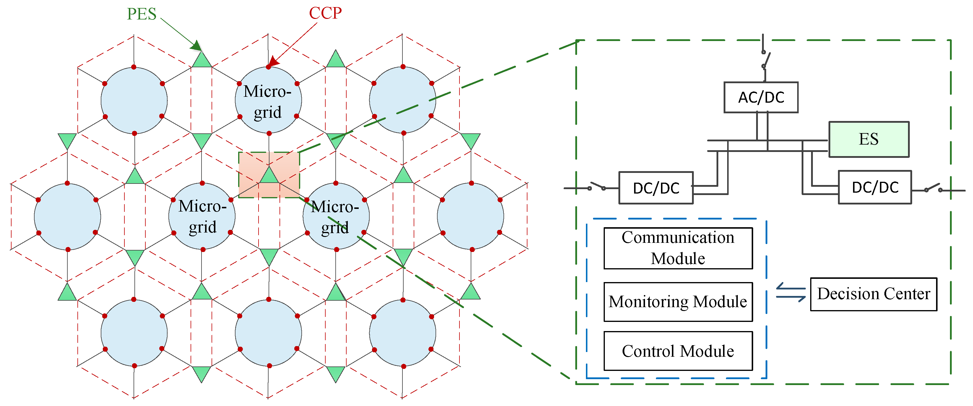
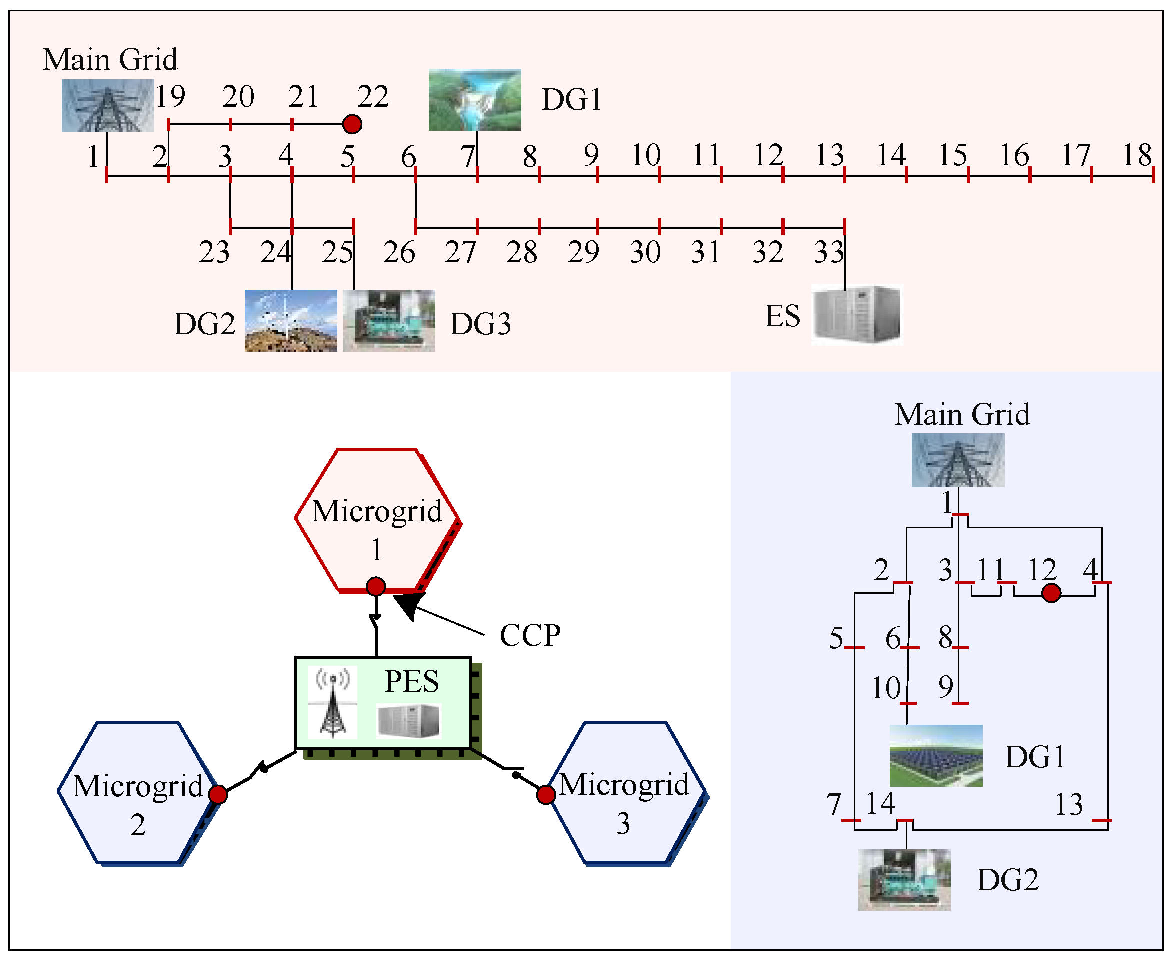
For PESs, the dispatchable element is the ESs in the PESs and the adjacent microgrid’s exchange power. The size of the exchange power in the study was the maximum delivery power of the ESs, $P_{PES}$. The carbon intensities of the CCPs of three microgrids connected to the PESs are $e_{CCPi}$, $e_{CCPj}$, $e_{CCPk}$; the carbon intensity of the PES is $e_{PES}$. The size of the power transfer from the PES to the microgrid i is $K_i*P_{PES}$; the transmission factor $K_i$ is calculated using Equation (11).

$$K_i=\left\{\begin{array}{cc}1,\hfill & e_{CCPi}>e_{PES}\hfill \\ -1,\hfill & e_{CCP}<e_{PES}and{e}_{CCPi}\le e_{CCPj}\le e_{CCPk}\hfill \\ 0,\hfill & e_{CCPi}=e_{PES}or{e}_{CCPjork}\le e_{CCPi}\le e_{PES}\hfill \end{array}\right.$$

(11)

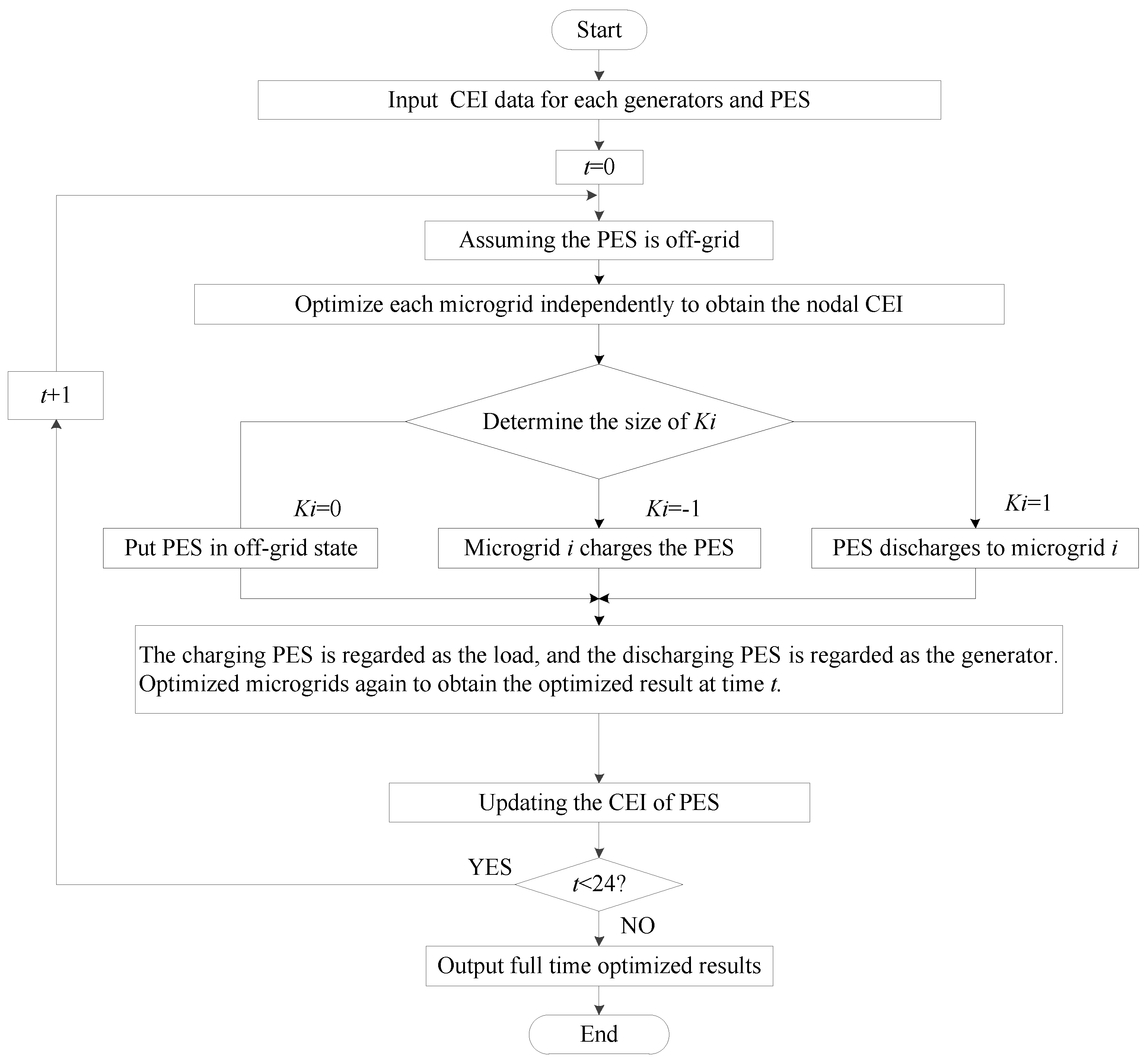
Based on the above two-part optimization scheme for microgrids and PESs, the overall HADN optimization process based on optimal carbon emission proposed in this paper is shown in Figure 2. The steps are as follows:

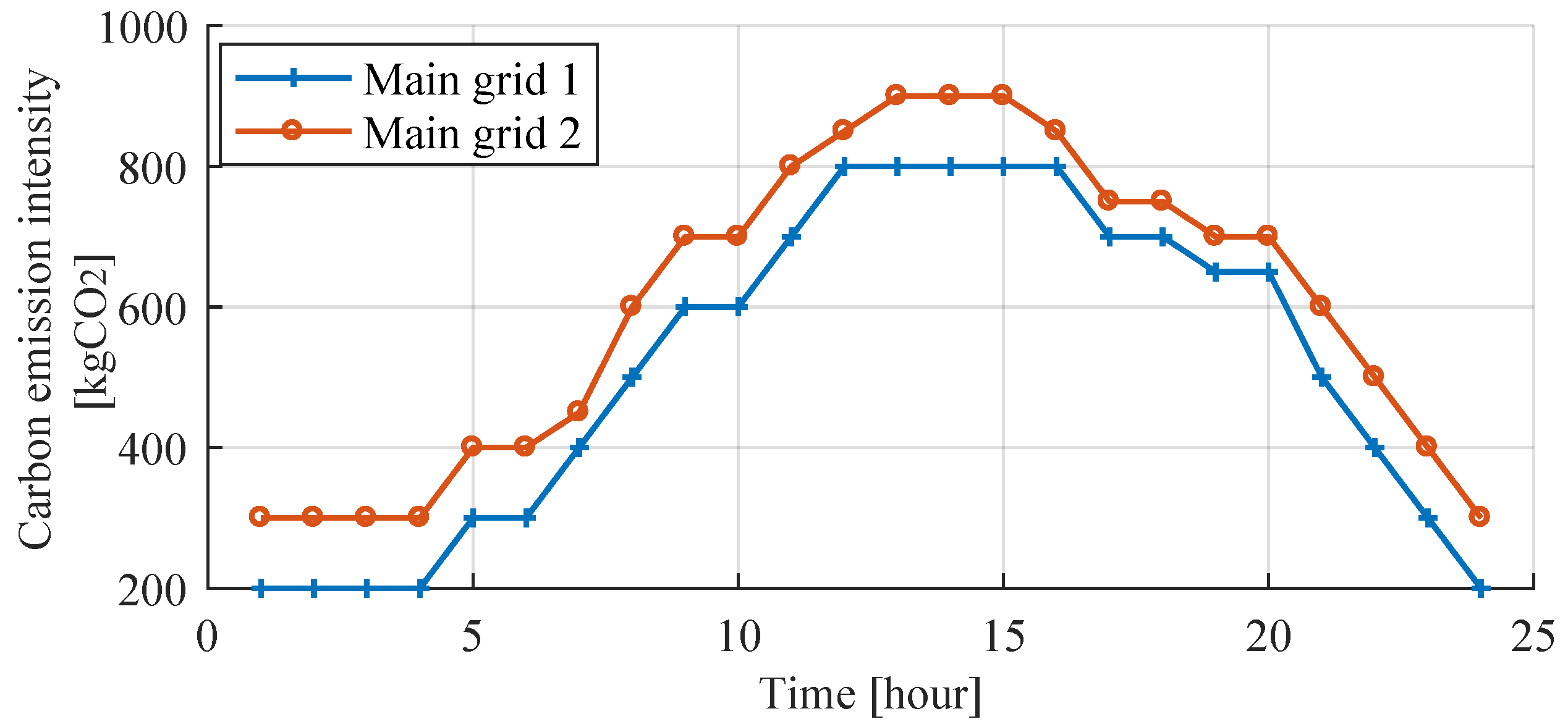
Step 1: Read the CEI of the main grid, DGs, and ESs within the microgrids, and the initial power and initial data of the ESs in the PESs at each time of the day.

Step 2: Enter the initial moment. First assume that each microgrid and the PES do not exchange electrical energy. Use general software to solve the above model and independently optimize each microgrid. Obtain the power output data of the main grid, DGs, and ESs in each microgrid.

Step 3: Calculate the CEI of each node within the microgrids based on the data obtained in step 2.

Step 4: Compare the discharge CEI of the ESs in the PESs, $e_{PES}$, with the CEI of the CCP of microgrid i, $e_{PCCi}$. Then, determine the power delivered by the PESs to microgrid i, $K_i*P_{PES}$. If $K_i$ = −1, the ESs of the PESs is regarded as a load connected to microgrid i. If $K_i$ = 1, the PES is regarded as a generator connected to microgrid i, and the CEI is the discharge CEI at this moment. If $K_i$ = 0, the PES is in the off-grid state and is not considered.

Step 5: Use the general software to solve the optimization model of each microgrid again. Then, obtain the power generated by the main grids and DGs, and the charging and discharging power of the ESs. Update the CEI data of the nodes of the system and calculate the system carbon emissions.

Step 6: Update the power and carbon flow data of the ESs in the microgrid and the ESs in the PESs for the next moment.

Step 7: If 24 time periods are reached, the optimization ends and the full-time optimization results are output; otherwise, return to step 3.

In summary, the tools for solving an optimization problem can be divided into three main classes: exact approaches, heuristics algorithms, and meta-heuristics algorithms. The features of these three kinds of methods are analyzed in detail below to highlight the contribution of this study.

(1) In exact approaches, mathematical models are usually developed using mathematical modeling methods, and the optimal solution to the problem is obtained by using optimization algorithms (simplex methods, branch-and-bound, branch-and-cut, etc.). They can be used to solve problems in common mathematical models, such as linear programming, integer programming, etc. CPLEX, GUROBI, FICO Xpress, SCIP, etc., can be used to solve these problems, which greatly reduce the solution time.

(2) Heuristics algorithms are problem-oriented procedures but cannot possible to find the optimal solution in a limited amount of time as the problem size increases. This requires a trade-off between solution accuracy and computing time. For large-scale problems, we do not need to find the optimal solution, but only a suboptimal solution or a satisfactory solution in a short period of time. Heuristic algorithms include the construction and improvement algorithms.

(3) Meta-heuristics algorithms are usually applied to a wider range of aspects using a general heuristic strategy without resorting to certain problem-specific conditions. They have some requirements for the search process and can use certain operations to jump out of the local optimum. In general, at least one initial feasible solution needs to be provided to efficiently search in a predefined search space. Meta-heuristics algorithms include simulated annealing, genetic algorithm, grey wolf optimizer, and Harris hawk optimizer.

A comparison of these three types of methods is summarized in

Table 3. Comparison of three types of methods.

Method	Typical Algorithms	Advantages	Disadvantages
Exact approaches	Simplex algorithm, branch-and-bound, branch-and-cut (use solver such as CPLEX)	Accurate optimal solution	Slow in solvin large-scale problems
Heuristics algorithm	Construction algorithm, improvement algorithm	Fast operation speed	Probably not the optimal solution
Meta-heuristics algorithm	Genetic algorithm, grey wolf optimizer, Harris hawk optimizer	Wide application and high global search capability	Initial feasible solution and parameter selection are required

.

From the above analysis, we concluded that with the CPLEX solver, strict optimal solutions can be quickly obtained. This feature makes the proposed method much more effective than other optimization methods. As mentioned above, the heuristic and meta-heuristic solving methods were designed for dealing with a very complex optimization problems with a trade-off between solving precision and solving speed. However, the developed model is for addressing linear programming problems; therefore, even for a large-scale problem, CPLEX can quickly solve the problem. Furthermore, there are some equality constraints in the developed model that lead to the need to constantly consider these constraints during the iterative process, and even the need to add measures such as penalty functions, which greatly increase the solving workload. Therefore, in this study, CPLEX was chosen to solve the model, which made it possible to accurately obtain the optimal solution in a very reasonable amount of solution time, and CPLEX is easy to use, avoiding the need to process the constraints or specifically select the relevant parameters.

4. Numerical Evaluation

4.1. Case Study

In this section, a case study is used to verify the proposed optimization method. Because the HADN is a new topology proposed in recent years, and there is no standard test system yet, a test system was built in this study based on the features and requirements of the supported project. The structure of the test system is shown in Figure 3, which is a HADN composed of three typical microgrids and one PES.

Microgrid 1 is a modified IEEE 33-bus system [30] in which three DGs and one ES are added to format an autonomous grid. The CCP in microgrid 1 was set as node 22. Microgrids 2 and 3 are both DC grids, which are transformed from the IEEE 14-bus system [31], and two DGs are added to both systems. The CCPs in microgrids 2 and 3 was set as as node 12. The branch conductance, node power, and node voltage of the three microgrids are shown in

Table 4. Parameters of microgrid 1.

Node i	Node j	Resistance ($\mathsf{\Omega }$)	Reactance (h)	Load of j (MW)	Node i	Node j	Resistance ($\mathsf{\Omega }$)	Reactance (h)	Load of j (MW)
1	2	0.0922	0.047	0.1 + 0.06i	2	3	0.493	0.2511	0.09 + 0.04i
3	4	0.366	0.1864	0.12 + 0.08i	4	5	0.3811	0.1941	0.06 + 0.03i
5	6	0.819	0.707	0.6 + 0.02i	6	7	0.18772	0.6188	0.2 + 0.1i
7	8	0.7114	0.2351	0.2 + 0.1i	8	9	1.03	0.74	0.06 + 0.02i
9	10	1.044	0.74	0.06 + 0.02i	10	11	0.1966	0.065	0.045 + 0.03i
11	12	0.3744	0.1238	0.06 + 0.035i	12	13	1.468	1.155	0.12 + 0.08i
13	14	0.5416	0.7129	0.06 + 0.01i	14	15	0.591	0.526	0.06 + 0.01i
15	16	0.7463	0.545	0.06 + 0.01i	16	17	1.289	1.721	0.06 + 0.02i
17	18	0.732	0.574	0.09 + 0.04i	2	19	0.164	0.1565	0.09 + 0.04i
19	20	1.5042	1.3554	0.09 + 0.04i	20	21	0.4095	0.4784	0.09 + 0.04i
21	22	0.7089	0.9373	0.09 + 0.04i	3	23	0.4512	0.3083	0.09 + 0.05i
23	24	0.898	0.7091	0.42 + 0.2i	24	25	0.896	0.7011	0.42 + 0.2i
26	27	0.2842	0.1447	0.06 + 0.025i	6	26	0.203	0.1034	0.06 + 0.025i
28	29	0.8042	0.7006	0.12 + 0.07i	27	28	1.059	0.9337	0.06 + 0.02i
30	31	0.9744	0.963	0.15 + 0.07i	29	30	0.5075	0.2585	0.2 + 0.6i
31	32	0.3105	0.3619	0.21 + 0.1i	32	33	0.341	0.5302	0.06 + 0.04i

Note: i represents the imaginary part of the plural.

and

Table 5. Parameters of microgrids 2 and 3.

Node i	Node j	Resistance ($\mathsf{\Omega }$)	Load of j (MW)	Node i	Node j	Resistance ($\mathsf{\Omega }$)	Load of j (MW)
1	2	0.3968	0.2	8	10	0.5819	0.45
1	3	0.5818	0.4	3	11	0.5818	0.1
1	4	0.5818	0.1	4	12	0.4762	0.1
2	5	0.4762	0.2	4	13	0.4232	0.1
2	6	0.4232	0.3	13	14	0.2116	2.1
5	7	0.2116	0.15	6	10	0.2115
3	8	0.4232	0.5	11	12	0.2115
8	9	0.5232	0.06	7	14	0.4761

. The parameters of all power sources in each microgrid are shown in

Table 6. Operating parameters of sources in microgrids.

Microgrid	Source	Node	CEI (kgCO2/kWh)	Pmax (kW)	Pmax (kW)
Microgrid 1	Main grid 1	1	Figure 4	4000	0
	DG1	7	0.55	650	0
	DG2	24	0.60	600	0
	DG3	25	0.65	1500	0
	ES	33	0.7 (initial)	50	−50
Microgrid 2	Main grid 1	1	Figure 4	4000	0
	DG1	10	0.55	800	0
	DG2	14	0.65	1000	0
Microgrid 3	Main grid 2	1	Figure 4	4000	0
	DG1	10	0.55	50	0
	DG2	14	0.65	600	0

.

Although the actual scenario may be different, in this simulation, a reasonable set of data was used for the calculation. The CEIs of the main grids 1 and 2 for 24 h are shown in Figure 4. The capacity of the ESs in the PESs was 100 kW, and the power conversion efficiency was 75% for both charging and discharging. The maximum storage power was $10,000$ kWh. In the initial state, the state of energy storage unit was set to $10\%$, the carbon flow contained was 300 kgCO${}_2$, and the equivalent discharge CEI was $0.4$ kgCO${}_2$/kWh.

The carbon emissions of the original microgrids without DGs, ESs, and PESs, $E\left(T\right)$, were calculated from the CEI of the main grid, $e_{MG}\left(T\right)$ and load power, $P_{LOAD}$ using Equation (12). The carbon emissions at all times of the day are shown in Figure 5; the total carbon emitted in one day was $123,328.1$ kgCO${}_2$.

$$E\left(T\right)=e_{MG}\left(T\right)P_{LOAD}$$

(12)

4.2. Optimization Dispatch Solutions

The proposed optimization method was implemented within Matlab, and the CPLEX solver was used to solve the optimization model.

4.2.1. Dispatch within Microgrids

The internal power scheduling scheme of the microgrids is illustrated in Figure 6. The data provided through the optimization that can be dispatched by the microgrids are as follows: The physical quantities to be dispatched include the power injected into microgrid 1 by the superior main grid 1, $P_{MG1\_1}$; the power emitted by the DGs and ESs inside microgrid 1, $P_{GEN1\_1}$, $P_{GEN1\_2}$, $P_{GEN1\_3}$, and $P_{ES1}$; the power injected into microgrid 2 by main grid 1, $P_{MG1\_2}$; the power emitted by the DGs inside microgrid 2, $P_{GEN2\_1}$ and $P_{GEN2\_2}$; the power injected into microgrid 3 by main grid 2, $P_{MG2}$; and the power emitted by the DGs inside microgrid 2, $P_{GEN3\_1}$ and $P_{GEN3\_2}$.

As can be seen in Figure 6, the low-carbon periods of the main grids are 1–7 h and 22–24 h, and the CEIs of the DGs and ESs are higher than those of the main grids. The power required by the loads are completely provided by the main grids, while the DGs do not contribute. The ESs are regarded as a load that absorb the low-carbon power at this time; their CEIs change with charging time. When the main grids enter a high-carbon period, 8–21 h, the carbon emission intensities of the DGs and ESs are lower than those of the main grids. The power required is given priority by the DGs with low carbon intensity, and the power output size is arranged according to the CEI and the upper and lower limits of th constraints. The ES is regarded as the power generator to release the low-carbon power previously absorbed.

4.2.2. Dispatch between Microgrids and PESs

The total power output for each period in Figure 6 is not equal, not only due to the process of the charging and discharging states of the ESs inside microgrid 1, but also due to the power exchanged between microgrids and PESs.

Table 7. The values of the transmission factors $K_1$, $K_2$, and $K_3$.

	Time
	1	2	3	4	5	6	7	8	9	10	11	12	13	14	15	16	17	18	19	20	21	22	23	24
$K_1$	−1	−1	−1	−1	−1	-1	1	1	1	1	1	1	1	1	1	1	1	1	1	1	1	1	−1	−1
$K_2$	0	0	0	0	0	0	1	1	1	1	1	1	1	1	1	1	1	1	1	1	1	1	0	0
$K_3$	0	0	0	1	1	1	1	1	1	1	1	1	1	1	1	1	1	1	1	1	1	1	0	0

shows the values of the transmission factors, $K_1$, $K_2$, and $K_3$ for the 24 time periods, which determine the charging and discharging states of the PESs.

Figure 7 illustrates the power delivered from the PESs to microgrids 1, 2 and 3 based on $K_i$, and the CEI of the ESs of the PESs, which change with the power delivery process.

At 1–6 h and 23–24 h, the CEI of the CCP of microgrid 1 is the lowest and less than that of the PESs, so microgrid 1 charges the PESs. The CEI of the PESs continuously decreases in this charging process.

At 4 h, because the CEI of the CCP of microgrid 3 is the first to be higher than that of the PESs, the PESs discharge to microgrid 3 at this time. The CEI of the PESs remains constant.

At 7–22 h, the main grid enters a high-carbon period, and the CEIs of microgrids 1, 2, and 3 are all higher than those of the PESs, so the ESs in the PESs are reset to the discharging state, and discharge to all the microgrids. The discharging CEI of the ESs in the PESs is recalculated according to Equation (1).

Considering the conversion efficiency of the charging and discharging processesof ESs, $\eta$, the charging CEI of the PES rises for a period of time at the beginning of charging, and then slowly falls according to the CEI of the microgrids. In this case study, the CEI of the PES tended to gradually decrease and converged to the lowest CEI of the microgrid that charged it.

4.3. Results and Discussion

In order to verify the validity and superiority of the proposed method, we adopted a comparative approach to our discussion. The structure and optimization models of the three systems were organized as shown in

Table 8. Three types of systems.

	Structure	Optimal Model
System 1	Original microgrids	Not applicable
System 2	Original microgrids with DGs accessed	Only consider power output from main grids and DGs in microgrids
System 3	Original microgrids with DGs accessed and connected by PES (HADN)	Consider power flow between microgrids and PES on basis of model 2

. System 1 was the most primitive microgrid, all load power was provided by the main grids, and no optimization conditions were available. In system 2, DGs were on the basis of system 1, all load power was provided by the main grids and DGs, and the optimization model needed to consider the power from the main grids and DGs, which were optimized by the method proposed by [28]. System 3 was the test system in this study, i.e., a typical HADN that was optimized by the method proposed in this paper. The comparison of carbon emissions for the three systems is shown in Figure 8. The color blocks in the figure are divided into the low- and high-carbon periods of the main grids.

Figure 9 provides further details on the two kinds of time periods. We selected 2–3 h as a typical low-carbon period of the main grid, as shown in the first line of the figure. Because the CEI of the main grid was low in this period, the ESs in the microgrid and the ESs in the PESs were treated as loads absorbing electricity, which was equivalent to an increase in the total load. So, the carbon emissions of system 3 were slightly larger than those of systems 1 and 2 at this time. We selected 12–13 h as a typical high-carbon period of the main grid, as shown in the second line in the figure. Because the ESs stored low-carbon power from the previous low-carbon period of the main grid, its CEI was much lower than at 0 h, the ESs acted as low-carbon distributed power sources and delivered power to the microgrid. The main grid with a high CEI sent out less power, so most of the power required by the load was generated by DGs and ESs. In the low-carbon period in the main grid, the carbon emission of system 3 was at most 30 kgCO${}_2$ more than that of system 1, but in the main grid in high-carbon period, such as 13 h, the carbon emission of system 3 was almost 2000 kgCO${}_2$ less than that of system 1.

The comparison of the three systems is summarized in

Table 9. Comparison of the three systems.

DG	PES	Carbon Emissions (kgCO${}_2$)	Ability to Control Carbon Emissions
×	×	123,328.1	None
✓	×	117,688	Weak
✓	✓	110,958	Strong

.

The total carbon emissions of system 1 was calculated as $123,328.1$ kgCO${}_2$ throughout the day. When the system line parameters and load size were determined, the carbon emission was only related to the CEI of the power injected into the system by the main grid. System 1 did not have the to control carbon emissions.

However, emphasizing the green sustainability of power grids, DG technology is developing, and DGs are increasingly being connected to grids. Grids of the system 1 type are gradually being replaced by those of the system 2 type, so system 2 has started to become the most common grid structure. The total carbon emission of system 2 was $117,688$ kgCO${}_2$, which was related to the sources of power. The system showed a certain flexibility in regulating carbon emissions because of its ability to dispatch the power output of the main grid and the DGs.

The total carbon emission of system 3 (HADN) was calcualted as $110,958$ kgCO${}_2$ for the whole day. The HADN is different from the distributed system, which is directly connected by microgrids, but uses PESs to connect the microgrids. The carbon emissions were not only related to the source of power from the main grids and DGs inside the microgrids, but also to the power exchanged through the PESs. So, the emissions could be adjusted by reasonably arranging the power output of the main grid and DGs. At the same time, the PES, as an additional ES with a scheduling function, can exchange low-carbon electricity between the microgrids.

We concluded that the total carbon emissions of system 3 were the lowest, although the emissions were higher than those of systems 1 and 2 during the main grid high-carbon period. This small increase in carbon emissions was insignificant compared with the total carbon emissions for the whole day. Additionally, as the CEI of the main grid continued to rise, the effects and advantages of HADN low-carbon optimization dispatch became more prominent.

The direction of electrical energy flow from microgrids to the PESs in the HADN is determined by the transmission factors, which can be artificially altered. The integration of PESs increased the grid flexibility to enable the dispatch of low-carbon emissions. The optimization objective in this study was to minimize the overall carbon emissions of the system, so the decision scheme for the transmission factors follows the rule of transferring electricity from low- to high-CEI microgrids. Each microgrid can make full use of the low-carbon power from the neighboring microgrids, while each microgrid operates in low-carbon status.

4.4. Practical Application Outlooks

This optimization of dispatch can be achieved by sending a command to the HADN-integrated regulation center. Thus, PESs can quickly and effectively, change the power flow between microgrids, and can issue scheduling instructions to neighboring microgrids in a more timely manner. In practice, different transmission rules can be formulated according to the different characteristics of the carbon emission responsibilities of each region. For example, microgrid 1 acted as a charging station for the PESs in this case study because it had the lowest CEI. If the general transmission rules are followed all the time, microgrid 1 will place considerable pressure on low-carbon sustainable development, so the transmission factors need to be adjusted to appropriately increase the priority of the other microgrids. As a result, a scheduling strategy more suitable for coordinated, regional, low-carbon development will be achieved.

Although this low-carbon optimization dispatch of a HADN has a number of advantages, it also faces many challenges in practical situations, as follows:

(1) Applicability in practical situations

Our case study considered an idealized situation: it did not take into account the possible lack of energy supply, degradation of energy storage components, or power outages. Therefore, in practical applications, it is necessary to more comprehensively consider the optimization objectives and to formulate reasonable constraints according to the actual grid conditions. One of the most unique optimization ideas in this study is that the power flow through PESs is based on the transmission factors. This idea can also be applied to other optimization objective dispatches: the only change required is to simply send a command to the integrated control center in the PESs to control the judgment rules of the transmission factors.

(2) Economic issues

In order to achieve distribution autonomy, many PESs are required for HADN, and given the current development status and the price of power semiconductors, it is possible that their construction cost would account for a high percentage of the total. So, the technical cost of building HADNs must be comprehensively considered. However, in the long term, with the further development of power semiconductor technology, the cost of power electronic devices that constitute the PESs is bound to gradually decrease, and coupled with the scale effect, there is reason to think that the construction costs of HADNs will gradually drop to an acceptable range. Additionally, HADNs have stronger and more flexible DER consumption capability, which is especially conducive to the distributed access and consumption of more new energy in the future, thus reducing power abandonment, compensating for the construction cost of PESs, and improving the overall economic benefits of the distribution grid.

(3) Technical issues

First, the requirements are high regarding the autonomous capability of microgrids and the autonomous operation of PESs. The basic idea of HADNs is to significantly reduce the operational control and dispatch complexity at the distribution network level by increasing the decision freedom between the PESs and the microgrids. The PESs must autonomously reach agreements and complete power dispatch with the associated microgrid based on the principle of competitive power market trading. The distribution network level thus only needs to supervise the PES sand issue them the priority of the execution of regulation instructions only when necessary. Second, the presence of PESs increases the number of variable current devices in the distribution network. The parallel operation of multiple inverters is prone to the ring current phenomenon and increases the network loss when the output voltage parameters are inconsistent, which is a problem that must be considered and studied in power system applications. At present, a variety of approaches have been proposed for ring current suppression, such as using the virtual impedance method, adding grid-connected transformers, and improving control strategies, all of which have achieved certain results. How to effectively further suppress the circulating current problem in HADNs is also a topic worthy of study in the future. Last, in HADNs, the operation control of each microgrid is relatively independent, so its relaying protection can also be relatively independently configured. However, because the microgrids are interconnected through PESs, each microgrid is equivalent to a multiple power supply mode, so the configuration of its relaying protection is more complicated than that of a traditional distribution network with open-loop operation, which needs further study.

The optimization method designed in this study verified the excellent low-carbon performance of HADNd and provides an idea for the flexible and optimal scheduling of HADNs. With further research and the application of new technologies, the problems above will be overcome one-by-one.

5. Conclusions

We designed an optimization dispatch model with the objective of minimizing the carbon emissions of HADNs. The CEF concept was introduced for measuring the carbon emissions of the system, so the output of power generators with different CEIs were accurately allocated and the carbon emissions of the different microgrids in different regions were clearly described. Transmission factors were introduced to address the problem of electric energy flow between PESs and neighboring microgrids. The transmission factors can be changed according to the optimization target in a timely manner to manipulate the power flow, highlighting the unique advantages of HADNs: regional autonomy and wide area interconnection. The mutual promotion of low-carbon undertakings between microgrids in each region was realized. In this study, the factors were determined by the CEI of each microgrid, so it could decide the direction of power from different microgrids and PESs to achieve the low-carbon target. The values of the transmission factors were determined by comparing the CEIs of the microgrids and PESs, thus regulating the energy flow between the microgrids and PESs. More profoundly, if the dispatching is carried out with other indicators, such as operation cost and power quality, the transmission factors can also be used to achieve mutual benefits among microgrids, which greatly improves the flexibility of the optimization of the dispatching of HADNs.

A HADN case study was conducted to explore the effectiveness of the proposed optimization method, and we analyzed the low-carbon performance of the HADN. The scheduling results within the microgrids showed that the power supply could be scheduled according to the CEI to produce the least carbon emissions within the microgrid. During the low-carbon periods for the main grid, the load power could be fully supplied by the main grid. As the CEI of main grid rose, the DGs with low CEI began to generate power. The optimization results of the system including both microgrids and PES showed that the HADN not only had the ability to dispatch low-carbon within each microgrid, but could also fully interact with low-carbon power between the different microgrids through the PESs to achieve the low-carbon operation of the whole system.

The observation from our case study was that although the addition of the charging ESs increased the total system load from the initial 13,755 to 13,905 $\mathrm{kWh}$ during the low-carbon periods of the main grid, the duration was short and the increase in carbon emissions was small. Moreover, due to the absorption of low-carbon electricity by the ES during this period, the CEI of the PES decreased from the initial 0.4 to 0.3795 $\mathrm{kgC}{\mathrm{O}}_2/\mathrm{kWh}$, and started to discharge at this CEI during high-carbon period of the main grid. In the end, the carbon emissions of systems 1, 2, and 3 (HADN case study) were 2343 123,328.1, 117,688, and 110,958 kgCO${}_2$, respectively. The comparison of these three cases showed that the addition of the DGs to the original microgrids resulted in a 4.6% reduction in the total carbon emissions; the addition of both DGs and PESs to the microgrids resulted in a 10.03% reduction in the total carbon emissions.

It is important to note that the presented results were obtained under the mentioned assumptions and should be interpreted accordingly. Additionally, several dimensions of this study should be further explored in the future. One direction is to study the changes in this optimization by expanding the range of the HADN system and increasing the load to to adapt to the pace of industrial development. Another suggestion is to consider the investment and operating costs while reducing carbon emissions, making the optimization dispatch more conducive to sustainable regional economic development. There are still many technical issues that need to be addressed in order to more effectively apply HADN optimization. Nevertheless, this study provides the verification of the HADN’s superior low-carbon performance, and lays the foundation for more detailed low-carbon dispatching of HADN and even for optimization dispatching considering more optimization objectives.

References

1. Blaabjerg, F.; Teodorescu, R.; Liserre, M.; Timbus, A. Overview of Control and Grid Synchronization for Distributed Power Generation Systems. IEEE Trans. Ind. Electron. 2006, 53, 1398–1409. [Google Scholar] [CrossRef]
2. Teodorescu, R.; Liserre, M.; Rodriguez, P. Grid Converters for Photovoltaic and Wind Power Systems; John Wiley & Sons, Ltd.: Hoboken, NJ, USA, 2011. [Google Scholar]
3. Guerrero, J.M.; Blaabjerg, F.; Zhelev, T.; Hemmes, K.; Monmasson, E.; Jemei, S.; Comech, M.P.; Granadino, R.; Frau, J.I. Distributed Generation: Toward a New Energy Paradigm. IEEE Ind. Electron. Mag. 2010, 4, 52–64. [Google Scholar] [CrossRef]
4. Balaguer, I.J.; Lei, Q.; Yang, S.; Supatti, U.; Peng, F.Z. Control for Grid-Connected and Intentional Islanding Operations of Distributed Power Generation. IEEE Trans. Ind. Electron. 2011, 58, 147–157. [Google Scholar] [CrossRef]
5. Hatziargyriou, N.; Asano, H.; Iravani, R.; Marnay, C. Microgrids. IEEE Power Energy Mag. 2007, 5, 78–94. [Google Scholar] [CrossRef]
6. Lasseter, R.; Akhil, A.; Marnay, C.; Stephens, J.; Dagle, J.; Guttromsom, R.; Meliopoulous, A.S.; Yinger, R.; Eto, J. Integration of Distributed Energy Resources. The CERTS Microgrid Concept; Lawrence Berkeley National Laboratory: Berkeley, CA, USA, 2002. [Google Scholar]
7. Lasseter, R.; Paigi, P. Microgrid: A Conceptual Solution. In Proceedings of the 2004 IEEE 35th Annual Power Electronics Specialists Conference (IEEE Cat. No.04CH37551), Aachen, Germany, 20–25 June 2004. [Google Scholar]
8. Peng, W.C. Development and challenges of distributed generation, the microgrid and smart distributed system. Autom. Electr. Power Syst. 2010, 34, 10–14,23. [Google Scholar]
9. Jewell, W.T. Electric Industry Infrastructure for Sustainability: Climate Change and Energy Storage. In Proceedings of the 2007 IEEE Power Engineering Society General Meeting, Tampa, FL, USA, 24–28 June 2007; pp. 1–3. [Google Scholar] [CrossRef]
10. Zhu, N.; Jiang, D.; Hu, P.; Yang, Y. Honeycomb Active Distribution Network: A Novel Structure of Distribution Network and Its Stochastic Optimization. In Proceedings of the 2020 15th IEEE Conference on Industrial Electronics and Applications (ICIEA), Kristiansand, Norway, 9–13 November 2020; pp. 455–462. [Google Scholar] [CrossRef]
11. Wang, L.; Zu, G.; Xu, W.; Zhu, W.; Luo, F. Honeycomb Distribution Networks: Concept and Central Features. In Proceedings of the 2022 5th International Conference on Energy, Electrical and Power Engineering (CEEPE), Chongqing, China, 22–24 April 2022; pp. 629–633. [Google Scholar] [CrossRef]
12. Ruan, C.; Jiang, D.; Yang, Y.; Chen, J.; Chen, J.; Lu, Y.; Xu, F. Reliability Calculation Based on Honeycomb Distribution Grid. In Proceedings of the 2018 IEEE International Power Electronics and Application Conference and Exposition (PEAC), Shenzhen, China, 4–7 November 2018; pp. 1–6. [Google Scholar] [CrossRef]
13. Yan, Y.; Yu, B.; Zhu, D.; Geng, L.; Peng, Y.; Jiang, W. ES-VSC-MTDC based energy hub for honeycomb distribution network. In Proceedings of the 2021 IEEE Sustainable Power and Energy Conference (iSPEC), Nanjing, China, 23–25 December 2021; pp. 3355–3360. [Google Scholar] [CrossRef]
14. Xiao, X.; Hu, P.; Fang, Y.; Jiang, D.; Zhang, Y. A Control strategy for Honeycomb Distribution Network. In Proceedings of the 2020 Asia Energy and Electrical Engineering Symposium (AEEES), Chengdu, China, 29–31 May 2020; pp. 543–549. [Google Scholar] [CrossRef]
15. Yang, Y.; Jiang, D.; Ruan, C.; Chen, J.; Naixuan, Z. Distributed Optimal Scheduling Based on Honeycomb Active Distribution Grid. Electr. Power Constr. 2019, 40, 3. [Google Scholar]
16. Zhou, T.; Kang, C.; Chen, Q.; Chen, Q. Preliminary theoretical investigation on power system carbon emission flow. Autom. Electr. Power Syst. 2012, 36, 7. [Google Scholar]
17. Kang, C.; Zhou, T.; Chen, Q.; Wang, J.; Sun, Y.; Xia, Q.; Yan, H. Carbon Emission Flow From Generation to Demand: A Network-Based Model. IEEE Trans. Smart Grid 2015, 6, 2386–2394. [Google Scholar] [CrossRef]
18. Zhou, T.; Kang, C.; Chen, Q.; Chen, Q. Preliminary investigation on a method for carbon emission flow calculation of power system. Autom. Electr. Power Syst. 2012, 36, 49–54. [Google Scholar]
19. Zhou, T.; Kang, C.; Chen, Q.; Chen, Q. Analysis on distribution characteristics and mechanisms of carbon emission flow in electric power network. Autom. Electr. Power Syst. 2012, 36, 39–44. [Google Scholar]
20. Ma, R.; Yuan, S.; Qin, Z. Analysis on carbon emission flow of power system with uncertain wind power injection. Autom. Electr. Power Syst. 2014, 38, 124–129. [Google Scholar]
21. Kang, C.; Cheng, Y.; Sun, Y.; Zhang, N.; Meng, J.; Yan, H. Recursive Calculation Method of Carbon Emission Flow in Power Systems. Autom. Electr. Power Syst. 2017, 41, 7. [Google Scholar]
22. Li, Y.; Liu, Q.; Zhang, Z.; Liu, J. Algorithm of Carbon Emission Flow Based on Power Distribution. Power Syst. Technol. 2017, 41, 5. [Google Scholar]
23. Corso, G.; Di Silvestre, M.L.; Ippolito, M.G.; Riva Sanseverino, E.; Zizzo, G. Multi-objective long term optimal dispatch of Distributed Energy Resources in micro-grids. In Proceedings of the 45th International Universities Power Engineering Conference UPEC2010, Cardiff, UK, 31 August–3 September 2010; pp. 1–5. [Google Scholar]
24. Yuan, C.; Li, F.; Kuri, B. Optimal power generation mix towards an emission target. In Proceedings of the 2011 IEEE Power and Energy Society General Meeting, Detroit, MI, USA, 24–28 July 2011; pp. 1–7. [Google Scholar] [CrossRef]
25. Cui, M. Low Carbon Dispatch of Distribution Network Containing Microgrid Using Chaotic Ant Swarm. In Proceedings of the 2012 International Conference on Control Engineering and Communication Technology, Shenyang, China, 7–9 December 2012; pp. 818–821. [Google Scholar] [CrossRef]
26. Strnad, I.; Škrlec, D. An approach to the optimal operation of the microgrid with renewable energy sources and energy storage systems. In Proceedings of the Eurocon 2013, Zagreb, Croatia, 1–4 July 2013. [Google Scholar] [CrossRef]
27. Li, J.; Zhao, J. Low carbon unit commitment for power system with wind farms and carbon capture devices based on DE-BBO algorithm. In Proceedings of the International Conference on Renewable Power Generation (RPG 2015), Beijing, China, 17–18 October 2015; pp. 1–6. [Google Scholar] [CrossRef]
28. Zhou, T.; Kang, C. Research on low-carbon oriented optimal operation of distribution networks based on carbon emission flow theory. J. Glob. Energy Interconnect. 2019, 2, 3. [Google Scholar]
29. Li, Y.; Tang, W.; Wu, Q. Modified Carbon Trading Based Low-carbon Economic Dispatch Strategy for Integrated Energy System with CCHP. In Proceedings of the 2019 IEEE Milan PowerTech, Milan, Italy, 23–27 June 2019; pp. 1–6. [Google Scholar] [CrossRef]
30. Bhati, J.S. IEEE 33 BUS SYSTEM (LINE DATA & LOAD DATA). Available online: https://www.researchgate.net/publication/333798354_IEEE_33_BUS_SYSTEM_LINE_DATA_LOAD_DATA (accessed on 30 June 2019).
31. Yk, B. IEEE 14 Bus System. Available online: https://www.researchgate.net/publication/353452133_IEEE_14_Bus_System_Simulink_Model (accessed on 31 March 2014).
Figure 1. Structure of HADN.
Energies 15 07107 g001
Figure 2. System optimization flow chart.
Energies 15 07107 g002
Figure 3. Schematic diagram of the reference system.
Energies 15 07107 g003
Figure 4. Carbon flow intensity of the main grids.
Energies 15 07107 g004
Figure 5. Carbon emission of the original microgrids.
Energies 15 07107 g005
Figure 6. Power dispatch of power generators in microgrids.
Energies 15 07107 g006
Figure 7. Source of electrical power for PES and CEI of PES.
Energies 15 07107 g007
Figure 8. Comparison of carbon emissions of the three systems.
Energies 15 07107 g008
Figure 9. Comparison of typical periods of the three systems.
Energies 15 07107 g009